Convergence of Distributed Asynchronous Learning Vector Quantization Algorithms

Convergence of Distributed Asynchronous Learning Vector

Quantization Algorithms

Benoˆıt Patra∗ BENOIT.PATRA@UPMC.FR

LSTA

Universit´e Pierre et Marie Curie – Paris VI Tour 15-25, 4 place Jussieu

75252 Paris cedex 05, France

Editor: Gabor Lugosi

Abstract

Motivated by the problem of effectively executing clustering algorithms on very large data sets, we address a model for large scale distributed clustering methods. To this end, we briefly recall some standards on the quantization problem and some results on the almost sure convergence of the competitive learning vector quantization (CLVQ) procedure. A general model for linear distributed asynchronous algorithms well adapted to several parallel computing architectures is also discussed. Our approach brings together this scalable model and the CLVQ algorithm, and we call the resulting technique the distributed asynchronous learning vector quantization algorithm (DALVQ). An in-depth analysis of the almost sure convergence of the DALVQ algorithm is performed. A striking result is that we prove that the multiple versions of the quantizers distributed among the processors in the parallel architecture asymptotically reach a consensus almost surely. Furthermore, we also show that these versions converge almost surely towards the same nearly optimal value for the quantization criterion.

Keywords: k-means, vector quantization, distributed, asynchronous, stochastic optimization, scal-ability, distributed consensus

1. Introduction

Distributed algorithms arise in a wide range of applications, including telecommunications, dis-tributed information processing, scientific computing, real time process control and many others. Parallelization is one of the most promising ways to harness greater computing resources, whereas building faster serial computers is increasingly expensive and also faces some physical limits such as transmission speeds and miniaturization. One of the challenges proposed for machine learning is to build scalable applications that quickly process large amounts of data in sophisticated ways. Building such large scale algorithms attacks several problems in a distributed framework, such as communication delays in the network or numerous problems caused by the lack of shared memory. Clustering algorithms are one of the primary tools of unsupervised learning. From a practical perspective, clustering plays an outstanding role in data mining applications such as text mining, web analysis, marketing, medical diagnostics, computational biology and many others. Clustering is a separation of data into groups of similar objects. As clustering represents the data with fewer clusters, there is a necessary loss of certain fine details, but simplification is achieved. The popular

competitive learning vector quantization (CLVQ) algorithm (see Gersho and Gray, 1992) provides a technique for building reliable clusters characterized by their prototypes. As pointed out by Bottou and Bengio (1995), the CLVQ algorithm can also be viewed as the on-line version of the widespread Lloyd’s method (see Lloyd 2003, for the definition) which is referred to as batch k-means in Bottou and Bengio (1995). The CLVQ also belongs to the class of stochastic gradient descent algorithms (for more information on stochastic gradient descent procedures we refer the reader to Benveniste et al. 1990).

The analysis of parallel stochastic gradient procedures in a machine learning context has re-cently received a great deal of attention (see for instance Zinkevich et al. 2009 and McDonald et al. 2010). In the present paper, we go further by introducing a model that brings together the original CLVQ algorithm and the comprehensive theory of asynchronous parallel linear algorithms devel-oped by Tsitsiklis (1984), Tsitsiklis et al. (1986) and Bertsekas and Tsitsiklis (1989). The resulting model will be called distributed asynchronous learning vector quantization (DALVQ for short). At a high level, the DALVQ algorithm parallelizes several executions of the CLVQ method concurrently on different processors while the results of these algorithms are broadcast through the distributed framework asynchronously and efficiently. Here, the term processor refers to any computing in-stance in a distributed architecture (see Bullo et al. 2009, chap. 1, for more details). Let us remark that there is a series of publications similar in spirit to this paper. Indeed in Frasca et al. (2009) and in Durham et al. (2009), a coverage control problem is formulated as an optimization problem where the functional cost to be minimized is the same of the quantization problem stated in this manuscript.

Let us provide a brief mathematical introduction to the CLVQ technique and DALVQ algo-rithms. The first technique computes quantization scheme for d dimensional samples z1,z2, . . .

using the following iterations on a Rdκ_vector,

w(t+1) =w(t)₋εt+1H(zt+1,w(t)), t≥0.

In the equation above, w(0)_∈ Rdκ_{and the}ε_{tare positive reals. The vector H(z,w)is the opposite} of the difference between the sample z and its nearest component in w. Assume that there are

M computing entities, the data are split among the memory of these machines: zi₁,zi₂, . . ., where

i_{∈ {}1, . . . ,M_}. Therefore, the DALVQ algorithms are defined by the M iterations_{wi(t)_}∞_t=0, called versions, satisfying (with slight simplifications)

wi(t+1) =

M

∑

j=1

ai,j(t)wj(τi,j(t))₋εi_t+1H z_ti₊₁,wi(t), i_{∈ {}1, . . . ,M_}and t_≥0.

The time instants τi,j(t)_≥0 are deterministic but unknown and the delays satisfy the inequality

t₋τi,j(t)_≥0. The families_{ai,j(t)_}M

j=1define the weights of convex combinations.

As a striking result, we prove that multiple versions of the quantizers, distributed among the processors in a parallel architecture, asymptotically reach a consensus almost surely. Using the materials introduced above, it writes

wi(t)₋wj(t)_−−→

t→∞ 0, (i,j)∈ {1, . . . ,M}

2_{, almost surely (a.s.).}

most satisfactory almost sure convergence theorem for the CLVQ algorithm obtained by Pag`es (1997).

For a given time span, our parallel DALVQ algorithm is able to process much more data than a single processor execution of the CLVQ procedure. Moreover, DALVQ is also asynchronous. This means that local algorithms do not have to wait at preset points for messages to become available. This allows some processors to compute faster and execute more iterations than others, and it also allows communication delays to be substantial and unpredictable. The communication channels are also allowed to deliver messages out of order, that is, in a different order than the one in which they were transmitted. Asynchronism can provide two major advantages. First, a reduction of the synchronization penalty, which could bring a speed advantage over a synchronous execution. Sec-ond, for potential industrialization, asynchronism has greater implementation flexibility. Tolerance to system failures and uncertainty can also be increased. As in the case with any on-line algorithm, DALVQ also deals with variable data loads over time. In fact, on-line algorithms avoid tremendous and non scalable batch requests on all data sets. Moreover, with an on-line algorithm, new data may enter the system and be taken into account while the algorithm is already running.

The paper is organized as follows. In Section 2 we review some standard facts on the clustering problem. We extract the relevant material from Pag`es (1997) without proof, thus making our ex-position self-contained. In Section 3 we give a brief exex-position of the mathematical framework for parallel asynchronous gradient methods introduced by Tsitsiklis (1984), Tsitsiklis et al. (1986) and Bertsekas and Tsitsiklis (1989). The results of Blondel et al. (2005) on the asymptotic consensus in asynchronous parallel averaging problems are also recalled. In Section 4, our main results are stated and proved.

2. Quantization and CLVQ Algorithm

In this section, we describe the mathematical quantization problem and the CLVQ algorithm. We also recall some convergence results for this technique found by Pag`es (1997).

2.1 Overview

Let µ be a probability measure on Rd _{with finite second-order moment. The quantization} prob-lem consists in finding a “good approximation” of µ by a set ofκvectors ofRd _{called quantizer.} Throughout the document theκquantization points (or prototypes) will be seen as the components of a Rdκ_{-dimensional vector w= (w}

1, . . . ,wκ). To measure the correctness of a quantization scheme given by w, one introduces a cost function called distortion, defined by

Cµ(w) = 1 2

Z

Rd1min_≤ℓ≤κkz−wℓk

2_dµ(z).

Under some minimal assumptions, the existence of an optimal Rdκ_{-valued quantizer vector w}◦_∈ argmin_w

∈(Rd₎κCµ(w) has been established by Pollard (1981) (see also Sabin and Gray 1986, Ap-pendix 2).

that is, for every Borel subset A ofRd

µn(A) = 1

n

n

∑

i=1

1{zi∈A}.

Much attention has been devoted to the convergence study of the quantization scheme provided by the empirical minimizers

w◦_n∈argmin w∈(Rd₎κ

Cµn(w).

The almost sure convergence of Cµ(w◦n)towards minw_∈(Rd₎κCµ(w)was proved by Pollard (1981, 1982a) and Abaya and Wise (1984). Rates of convergence and nonasymptotic performance bounds have been considered by Pollard (1982b), Chou (1994), Linder et al. (1994), Bartlett et al. (1998), Linder (2001, 2000), Antos (2005) and Antos et al. (2005). Convergence results have been estab-lished by Biau et al. (2008) where µ is a measure on a Hilbert space. It turns out that the mini-mization of the empirical distortion is a computationally hard problem. As shown by Inaba et al. (1994), the computational complexity of this minimization problem is exponential in the number of quantizersκand the dimension of the data d. Therefore, exact computations are intractable for most of the practical applications.

Based on this, our goal in this document is to investigate effective methods that produce accurate quantizations with data samples. One of the most popular procedure is Lloyd’s algorithm (see Lloyd, 2003) sometimes refereed to as batch k-means. A convergence theorem for this algorithm is provided by Sabin and Gray (1986). Another celebrated quantization algorithm is the competitive learning vector quantization (CLVQ), also called on-line k-means. The latter acronym outlines the fact that data arrive over time while the execution of the algorithm and their characteristics are unknown until their arrival times. The main difference between the CLVQ and the Lloyd’s algorithm is that the latter run in batch training mode. This means that the whole training set is presented before performing an update, whereas the CLVQ algorithm uses each item of the training sequence at each update.

The CLVQ procedure can be seen as a stochastic gradient descent algorithm. In the more general context of gradient descent methods, one cannot hope for the convergence of the procedure towards global minimizers with a non convex objective function (see for instance Benveniste et al. 1990). In our quantization context, the distortion mapping Cµis not convex (see for instance Graf and Luschgy 2000). Thus, just as in Lloyd’s method, the iterations provided by the CLVQ algorithm converge towards local minima of Cµ.

Assuming that the distribution µ has a compact support and a bounded density with respect to the Lebesgue measure, Pag`es (1997) states a result regarding the almost sure consistency of the CLVQ algorithm towards critical points of the distortion Cµ. The author shows that the set of critical points necessarily contains the global and local optimal quantizers. The main difficulties in the proof arise from the fact that the gradient of the distortion is singular onκ-tuples having equal components and the distortion function Cµis not convex. This explains why standard theories for stochastic gradient algorithm do not apply in this context.

2.2 The Quantization Problem, Basic Properties

C : Rdκ_−→[0,∞)defined by

C(w),1

2

Z

G1min≤ℓ≤κkz−wℓk

2_{dµ(z), w= (w}

1, . . . ,wκ)∈

Rdκ_.

Throughout the document, with a slight abuse of notation, _k._kmeans both the Euclidean norm of Rd _or Rdκ_{. In addition, the notation}

_D

κ

∗ stands for the set of all vector of Rd κ

with pairwise distinct components, that is,

D

_∗κ,n_w∈Rd

κ

|wℓ6=wkif and only ifℓ6=k

o .

Under some extra assumptions on µ, the distortion function can be rewritten using space partition set called Vorono¨ı tessellation.

Definition 1 Let w_∈ Rdκ_{, the Vorono¨ı tessellation of}

_G

_{related to w is the family of open sets}

{Wℓ(w)}1≤ℓ≤κdefined as follows:

• If w_∈

D

_∗κ, for all 1_≤ℓ_≤κ,

Wℓ(w) =

v_∈

G

kwℓ−vk<min

k₆=ℓkwk−vk

.

• If w_∈ Rdκ_\

_D

κ

∗, for all 1≤ℓ≤κ,

– ifℓ=min_{k_|wk=wℓ},

Wℓ(w) =

v_∈

G

kwℓ−vk< min

wk6=wℓk wk−vk

– otherwise, Wℓ(w) =/0.

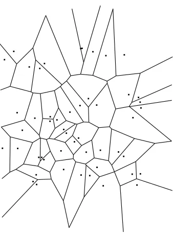
As an illustration, Figure 1 shows Vorono¨ı tessellations associated to a vector w lying in([0,1]_× [0,1])50 _{whose components have been drawn independently and uniformly. This figure also} high-lights a remarkable property of the cell borders, which are portions of hyperplanes (see Graf and Luschgy, 2000).

Observe that if µ(H)is zero for any hyperplane H ofRd_{(a property which is sometimes referred} to as strong continuity) then using Definition 1, it is easy to see that the distortion takes the form:

C(w) = 1 2

κ

∑

ℓ=1

Z

Wℓ(w)k

z₋wℓk2dµ(z), w∈

Rdκ_.

The following assumption will be needed throughout the paper. This assumption is similar to the peak power constraint (see Chou 1994 and Linder 2000). Note that most of the results of this subsection are still valid if µ satisfies the weaker strong continuity property.

Assumption 1 (Compact supported density) The probability measure µ has a bounded density

with respect to the Lebesgue measure onRd_{. Moreover, the support of µ is equal to its convex hull}

Figure 1: Vorono¨ı tessellation of 50 points ofR2_{drawn uniformly in a square.}

The next proposition states the differentiability of the distortion C, and provides an explicit formula for the gradient∇C whenever the distortion is differentiable.

Proposition 1 (Pag`es 1997) Under Assumption 1, the distortion C is continuously differentiable at

every w= (w1, . . . ,wκ)∈

D

_∗κ. Furthermore, for all 1≤ℓ≤κ, ∇ℓC(w) =

Z

Wℓ(w)(wℓ−z)dµ(z).

Some necessary conditions on the location of the minimizers of C can be derived from its dif-ferentiability properties. Therefore, Proposition 2 below states that the minimizers of C have parted components and that they are contained in the support of the density. Thus, the gradient is well defined and these minimizers are necessarily some zeroes of∇C. For the sequel it is convenient to

letA be the interior of any subset A of◦ Rdκ_.

Proposition 2 (Pag`es 1997) Under Assumption 1, we have

argmin w∈(Rd₎κ

C(w)_⊂argminloc w∈Gκ

C(w)_⊂

G

◦κ∩{∇C=0} ∩

D

_∗κ,

where argminloc_w∈GκC(w)stands for the set of local minimizers of C over

G

κ.

For any z_∈Rd_{and w∈} Rdκ_{, let us define the following vector of} Rdκ

H(z,w), _(wℓ−z)1

{z∈Wℓ(w)}

On

D

_∗κ, the function H may be interpreted as an observation of the gradient. With this notation, Proposition 1 states that

∇C(w) =

Z

GH(z,w)dµ(z), w∈

D

κ

∗.

Let∁A stands for the complementary in Rdκ_{of a subset A⊂} Rdκ_{. Clearly, for all w∈}∁

_D

κ

∗,

the mapping H(.,w)is integrable. Therefore,∇C can be extended on Rdκ_{via the formula}

h(w),Z

GH(z,w)dµ(z), w∈

Rdκ_{. (2)}

Note however that the function h, which is sometimes called the average function of the algorithm, is not continuous.

Remark 1 Under Assumption 1, a computation for all w_∈

D

_∗κof the Hessian matrix∇2C(w)can be deduced from Theorem 4 of (Fort and Pag`es, 1995). In fact, the formula established in this theorem is valid for cost functions which are more complex than C (they are associated to Kohonen Self Organizing Maps, see Kohonen 1982 for more details). In Theorem 4, lettingσ(k) =1_{k=0_},

provides the result for our distortion C. The resulting formula shows that h is singular on∁

D

_∗κand, consequently, that this function cannot be Lipschitz on

G

κ.

2.3 Convergence of the CLVQ Algorithm

The problem of finding a reliable clustering scheme for a data set is equivalent to find optimal (or at least nearly optimal) minimizers for the mapping C. A minimization procedure by a usual gradient descent method cannot be implemented as long as∇C is unknown. Thus, the gradient is

approximated by a single example extracted from the data. This leads to the following stochastic gradient descent procedure

w(t+1) =w(t)₋εt+1H(zt+1,w(t)), t≥0, (3) where w(0)_∈

G

◦κ∩

D

_∗κand z1,z2. . .are independent observations distributed according to the probability measure µ.

The algorithm defined by the iterations (3) is known as the CLVQ algorithm in the data analysis community. It is also called the Kohonen Self Organizing Map algorithm with 0 neighbor (see for instance Kohonen 1982) or the on-line k-means procedure (see MacQueen 1967 and Bottou 1998) in various fields related to statistics. As outlined by Pag`es in Pag`es (1997), this algorithm belongs to the class of stochastic gradient descent methods. However, the almost sure convergence of this type of algorithm cannot be obtained by general tools such as Robbins-Monro method (see Robbins and Monro, 1951) or the Kushner-Clark’s Theorem (see Kushner and Clark, 1978). Indeed, the main difficulty essentially arises from the non convexity of the function C, its non coercivity and the singularity of h at∁

D

_∗κ(we refer the reader to Pag`es 1997, Section 6, for more details).

The following assumption set is standard in a gradient descent context. It basically upraises constraints on the decreasing speed of the sequence of steps_{εt}∞t=0.

Assumption 2 (Decreasing steps) The (0,1)-valued sequence_{εt}t∞=0 satisfies the following two

1. ∑_t∞₌₀εt =∞.

2. ∑_t∞₌₀ε2_t <∞.

An examination of identities (3) and (1) reveals that if zt+1 ∈Wℓ0(w(t)), where the integer ℓ0∈ {1, . . . ,M}then

wℓ0(t+1) = (1−εt+1)wℓ0(t) +εt+1zt+1.

The component wℓ0(t+1)can be viewed as the image of wℓ0(t)by a zt+1-centered homothety with

ratio 1₋εt+1(Figure 2 provides an illustration of this fact). Thus, under Assumptions 1 and 2, the trajectories of_{w(t)_}t∞₌₀stay in

G

◦κ∩

D

_∗κ. More precisely, if

w(0)_∈

G

◦κ_∩

D

_∗κ

then

w(t)_∈

G

◦κ∩

D

_∗κ, t_≥0, a.s.

Figure 2: Drawing of a portion of a 2-dimensional Vorono¨ı tessellation. For t _≥0, if the vector zt+1∈Wℓ0(w(t))then wℓ(t+1) =wℓ(t)for allℓ6=ℓ0 and wℓ0(t+1)lies in the segment

[wℓ0(t),zt+1]. The update of the vector wℓ0(t) can also be viewed as a zt+1-centered

homothety with ratio 1−εt+1.

Although ∇C is not continuous some regularity can be obtained. To this end, we need to

in-troduce the following materials. For any δ>0 and any compact set L_⊂Rd_{, let the compact set}

Lκ_δ⊂ Rdκ_{be defined as}

L_δκ,

w_∈Lκ_|min

k6=ℓkwℓ−wkk ≥δ

. (4)

The next lemma that states on the regularity of∇C will prove to be extremely useful in the proof of

Lemma 2 (Pag`es 1997) Assume that µ satisfies Assumption 1 and let L be a compact set of Rd_.

Then, there is some constant P_δsuch that for all w and v in Lκ_δ with[w,v]_⊂

D

_∗κ,

k∇C(w)₋∇C(v)_{k ≤}P_δkw₋v_k.

The following lemma, called G-lemma in Pag`es (1997) is an easy-to-apply convergence results on stochastic algorithms. It is particularly adapted to the present situation of the CLVQ algorithm where the average function of the algorithm h is singular.

Theorem 3 (G-lemma, Fort and Pag`es 1996) Assume that the iterations (3) of the CLVQ

algo-rithm satisfy the following conditions:

1. ∑_t∞₌₁εt =∞andεt −−→ t_→∞ 0.

2. The sequences_{w(t)_}∞_t=0and_{h(w(t))_}t∞₌₀are bounded a.s. 3. The series∑∞_t=0εt+1(H(zt+1,w(t))−h(w(t)))converge a.s. in Rd

κ

.

4. There exists a lower semi-continuous function G : Rdκ_−→[0,∞_{)such that}

∞

∑

t=0

εt+1G(w(t))<∞, a.s.

Then, there exists a random connected componentΞof{G=0}such that

dist(w(t),Ξ)_−−→

t→∞ 0, a.s.,

where the symbol dist denotes the usual distance function between a vector and a subset of Rdκ_.

Note also that if the connected components of_{G=0_}are singletons then there existsξ_{∈ {}G=0_}

such that w(t)_−−→

t→∞ ξa.s.

For a definition of the topological concept of connected component, we refer the reader to Choquet (1966). The interest of the G-lemma depends upon the choice of G. In our context, a suitable lower semi-continuous function isG defined byb

b

G(w), _{lim inf}

v∈Gκ∩D_∗κ,v→wk∇C(v)k

2_{, w}

∈

G

κ. (5)

The next theorem is, as far as we know, the first almost sure convergence theorem for the stochastic algorithm CLVQ.

Theorem 4 (Pag`es 1997) Under Assumptions 1 and 2, conditioned on the event

n

lim inf

t→∞ dist w(t),

∁

_D

κ

∗

>0o, one has

dist(w(t),Ξ_∞)_−−→

t_→∞ 0, a.s.,

The proof is an application of the above G-lemma with the mappingG defined by Equation (5).b

Theorem 4 states that the iterations of the CLVQ necessarily converge towards some critical points (zeroes of∇C). From Proposition 2 we deduce that the set of critical points necessarily contains

optimal quantizers. Recall that without more assumption than w(0)_∈

G

◦κ∩

D

_∗κ, we have already discussed the fact that the components of w(t) are almost surely parted for all t _≥0. Thus, it is easily seen that the two following events only differ on a set of zero probability

n

lim inf

t_→∞ dist w(t),

∁

_D

κ

∗

>0o

and

inf

t_≥0dist w(t),

∁

_D

κ

∗

>0

.

Some results are provided by Pag`es (1997) for asymptotically stuck components but, as pointed out by the author, they are less satisfactory.

3. General Distributed Asynchronous Algorithm

We present in this section some materials and results of the asynchronous parallel linear algorithms theory.

3.1 Model Description

Let s(t)be any Rdκ_{-valued vector and consider the following iterations}

w(t+1) =w(t) +s(t), t_≥0. (6)

Here, the model of discrete time described by iterations (6) can only be performed by a single computing entity. Therefore, if the computations of the vectors s(t)are relatively time consuming then not many iterations can be achieved for a given time span. Consequently, a parallelization of this computing scheme should be investigated. The aim of this section is to discuss a precise mathematical description of a distributed asynchronous model for the iterations (6). This model for distributed computing was originally proposed by Tsitsiklis et al. (1986) and was revisited in Bertsekas and Tsitsiklis (1989, Section 7.7).

Assume that we dispose of a distributed architecture with M computing entities called processors (or agents, see for instance Bullo et al. 2009). Each processor is labeled, for simplicity of notation, by a natural number i_{∈ {}1, . . . ,M_}. Throughout the paper, we will add the superscript i on the variables possessed by the processor i. In the model we have in mind, each processor has a buffer where its current version of the iterated vector is kept, that is, local memory. Thus, for agent i such iterations are represented by the Rdκ_{-valued sequencew}i(t) ∞_t=0.

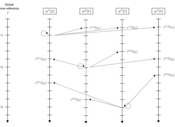
Let t _≥0 denote the current time. For any pair of processors (i,j)_{∈ {}1, . . . ,M_}2, the value kept by agent j and available for agent i at time t is not necessarily the most recent one, wj_(t), but more probably and outdated one, wj(τi,j_{(t)), where the deterministic time instant}τi,j_(t)satisfy 0_≤τi,j(t)_≤t. Thus, the difference t₋τi,j(t) can be seen as a communication delay. This is a modeling of some aspects of the network: latency and bandwidth finiteness.

analysis purposes. The processors work without knowledge of this global clock. They have access to a local clock or to no clock at all.

The algorithm is initialized at t =0, where each processor i_{∈ {}1, . . . ,M_} has an initial ver-sion wi(0)_∈ Rdκ_{in its buffer. We define the general distributed asynchronous algorithm by the} following iterations

wi(t+1) =

M

∑

j=1

ai,j(t)wj(τi,j(t)) +si(t), i_{∈ {}1, . . . ,M_}and t_≥0. (7)

The model can be interpreted as follows: at time t_≥0, processor i receives messages from other processors containing wj₍τi,j_{(t)). Processor i incorporates these new vectors by forming a convex} combination and incorporates the vector si(t) resulting from its own “local” computations. The coefficients ai,j(t)are nonnegative numbers which satisfy the constraint

M

∑

j=1

ai,j(t) =1, i_{∈ {}1, . . . ,M_}and t_≥0. (8)

As the combining coefficients ai,j_{(t)depend on t, the network communication topology is} some-times referred to as time-varying. The sequencesτi,j(t) ∞_t=0need not to be known in advance by any processor. In fact, their knowledge is not required to execute iterations defined by Equation (7). Thus, we do not necessary dispose of a shared global clock or synchronized local clocks at the processors.

As for now the descent termssi(t) _t∞₌₀will be arbitrary Rdκ_{-valued sequences. In Section 4,} when we define the distributed asynchronous learning vector quantization (DALVQ), the definition of the descent terms will be made more explicit.

3.2 The Agreement Algorithm

This subsection is devoted to a short survey of the results, found by Blondel et al. (2005), for a natural simplification of the general distributed asynchronous algorithm (7). This simplification is called agreement algorithm by Blondel et al. and is defined by

xi(t+1) =

M

∑

j=1

ai,j(t)xj(τi,j(t)), i_{∈ {}1, . . . ,M_}and t_≥0. (9)

where xi(0)_∈ Rdκ_{. An observation of these equations reveals that they are similar to iterations} (7), the only difference being that all descent terms equal 0.

In order to analyse the convergence of the agreement algorithm (9), Blondel et al. (2005) define two sets of assumptions that enforce some weak properties on the communication delays and the network topology. As shown in Blondel et al. (2005), if the assumptions contained in one of these two set hold, then the distributed versions of the agreement algorithm, namely the xi, reach an asymptotical consensus. This latter statement means that there exists a vector x⋆(independent of i) such that

xi(t)_−−→

t_→∞ x

⋆_{, i∈ {1, . . . ,M}.}

Global time reference

Figure 3: Illustration of the time delays introduced in the general distributed asynchronous algo-rithm. Here, there are M=4 different processors with their own computations of the vectors w(i), i_{∈ {}1,2,3,4_}. Three arbitrary values of the global time t are represented (t1,

t2and t3), withτi,i(tk) =tk for all i∈ {1,2,3,4}and 1≤k≤3. The dashed arrows head towards the versions available at time tkfor an agent i∈ {1,2,3,4}represented by the tail of the arrow.

3 essentially ensures, in its third statement, that the communication delays t₋τi,j(t)are bounded. This assumption prevents some processor from taking into account some arbitrarily old values com-puted by others processors. Assumption 3 1. is just a convention: when ai,j_{(t) =0 the value}τi,j_(t) has no effect on the update. Assumption 3 2. is rather natural because processors have access to their own most recent value.

Assumption 3 (Bounded communication delays)

1. If ai,j(t) =0 then one hasτi,j(t) =t, (i,j)_{∈ {}1, . . . ,M_}2and t_≥0,

2. τi,i(t) =t, i_{∈ {}1, . . . ,M_} and t_≥0.

3. There exists a positive integer B1such that

t₋B1<τi,j(t)≤t, (i,j)∈ {1, . . . ,M}2and t≥0.

Assumption 4 (Convex combination and threshold) There exists a positive constantα>0 such

that the following three properties hold:

1. ai,i(t)_≥α, i_{∈ {}1, . . . ,M_} and t_≥0.

2. ai,j(t)_{∈ {}0_{} ∪}[α,1], (i,j)_{∈ {}1, . . . ,M_}2 and t_≥0.

3. ∑M_j=1ai,j(t) =1, i_{∈ {}1, . . . ,M_} and t_≥0.

Let us mention one particular relevant case for the choice of the combining coefficients ai,j(t). Let i_{∈ {}1, . . . ,M_}and t_≥0, the set

Ni(t),_{j∈ {1, . . . ,M} ∈ {1, . . . ,M} |a}i,j_(t)

6

=0

corresponds to the set of agents whose version is taken into account by processor i at time t. For all (i,j)_{∈ {}1, . . . ,M_}2and t_≥0, the weights ai,j_{(t)are defined by}

ai,j(t) =

(

1/#Ni(t) if j_∈Ni(t); 0 otherwise;

where #A denotes the cardinal of any finite set A. The above definition on the combining coefficients appears to be relevant for practical implementations of the model DALVQ introduced in Section 4. For a discussion on others special interest cases regarding the choices of the coefficients ai,j(t)we refer the reader to Blondel et al. (2005).

The communication patterns, sometimes refereed to as the network communication topology, can be expressed in terms of directed graph. For a thorough introduction to graph theory, (see Jungnickel, 1999).

Definition 5 (Communication graph) Let us fix t≥0, the communication graph at time t,(

V

,E(t)), is defined by

• the set of vertices

V

is formed by the set of processors

V

=_{1, . . . ,M_},

• the set of edges E(t)is defined via the relationship

(j,i)_∈E(t)if and only if ai,j(t)>0.

Assumption 5 is a minimal condition required for a consensus among the processors. More pre-cisely, it states that for any pair of agents(i,j)_{∈ {}1, . . . ,M_}2there is a sequence of communications where the values computed by agent i will influence (directly or indirectly) the future values kept by agent j.

Assumption 6 (Bounded communication intervals) If i communicates with j an infinite number

of times then there is a positive integer B2such that

(i,j)_∈E(t)_∪E(t+1)_∪. . ._∪E(t+B2−1), t≥0.

Assumption 7 is a symmetry condition: if agent i_{∈ {}1, . . . ,M_}communicates with agent j_∈ {1, . . . ,M_}then j has communicated or will communicate with i during the time interval(t₋B3,t+

B3)where B3>0.

Assumption 7 (Symmetry) There exists some B3>0 such that whenever the pair (i,j)∈E(t),

there exists someτthat satisfies_|t₋τ_|<B3and(j,i)∈E(τ). To shorten the notation, we set

(AsY)_1≡

          

Assumption 3; Assumption 4; Assumption 5; Assumption 6.

(AsY)_2≡

          

Assumption 3; Assumption 4; Assumption 5; Assumption 7;

We are now in a position to state the main result of this section. The Theorem 6 expresses the fact that, for the agreement algorithm, a consensus is asymptotically reached by the agents.

Theorem 6 (Blondel et al. 2005) Under the set of Assumptions(AsY)₁or(AsY)₂, there is a con-sensus vector x⋆_∈ Rdκ_{(independent of i) such that}

lim t→∞

xi_(t)−x⋆_{=0, i∈ {1, . . . ,M}.}

Besides, there existρ∈[0,1)and L>0 such that

xi_(t)

−xi(τ)_≤Lρt−τ, i_{∈ {}1, . . . ,M_}and t_≥τ_≥0.

3.3 Asymptotic Consensus

This subsection is devoted to the analysis of the general distributed asynchronous algorithm (7). For this purpose, the study of the agreement algorithm defined by Equations (9) will be extremely fruitful. The following lemma states that the version possessed by agent i_{∈ {}1, . . . ,M_} at time

t_≥0, namely wi_{(t), depends linearly on the others initialization vectors w}j_{(0) and the descent} subsequencessj(τ) t_τ−₌1

−1, where j∈ {1, . . . ,M}.

Lemma 7 (Tsitsiklis 1984) For all (i,j)_{∈ {}1, . . . ,M_}2 and t_≥0, there exists a real-valued

se-quenceφi,j(t,τ) t_τ−₌1₋₁such that

wi(t) =

M

∑

j=1

φi,j_(t,

−1)wj(0) +

t−1

∑

τ=0 M

∑

j=1

φi,j_(t,τ)sj_(τ).

For all(i,j)_{∈ {}1, . . . ,M_}2and t≥0, the real-valued sequencesφi,j(t,τ) t_τ−₌1

−1do not depend on the value taken by the descent terms si(t). The real numbersφi,j(t,τ) are determined by the sequencesτi,j₍τ₎ t

τ=0and

ai,j₍τ₎ t

Lemma 8 (Tsitsiklis 1984) For all (i,j)_{∈ {}1, . . . ,M_}2, letφi,j(t,τ) t_τ−₌1

−1 be the sequences

de-fined in Lemma 7.

1. Under Assumption 4,

0_≤φi,j(t,τ)_≤1, (i,j)_{∈ {}1, . . . ,M_}2and t>τ_{≥ −}1. 2. Under Assumptions(AsY)₁or(AsY)₂, we have:

(a) For all(i,j)_{∈ {}1, . . . ,M_}2andτ_{≥ −}1, the limit ofφi,j(t,τ)as t tends to infinity exists and is independent of j. It will be denotedφi₍τ_).

(b) There exists someη>0 such that φi_{(τ)>η, i}

∈ {1, . . . ,M_}andτ_{≥ −}1.

(c) There exist a constant A>0 andρ_∈(0,1)such that

φi,j_(t,τ)

−φi(τ)_≤Aρt−τ, (i,j)_{∈ {}1, . . . ,M_}2and t>τ_{≥ −}1.

Take t′ _≥0 and assume that the agents stop performing update after time t′, but keep com-municating and merging the results. This means that sj(t) =0 for all t_≥t′. Then, Equations (7) write

wi(t+1) =

M

∑

j=1

ai,j(t)wj τi,j(t), i_{∈ {}1, . . . ,M_}and t_≥t′.

If Assumptions (AsY)₁ or (AsY)₂ are satisfied then Theorem 6 shows that there is a consensus vector, depending on the time instant t′. This vector will be equal to w⋆(t′) defined below (see Figure 4). Lemma 8 provides a good way to define the sequence_{w⋆(t)_}t∞₌₀as shown in Definition 9. Note that this definition does not involve any assumption on the descent terms.

Definition 9 (Agreement vector) Assume that Assumptions (AsY)₁ or(AsY)₂ are satisfied. The agreement vector sequence_{w⋆(t)_}∞_t=0is defined by

w⋆(t),

M

∑

j=1

φj₍

−1)wj(0) +

t₋1

∑

τ=0 M

∑

j=1

φj_(τ)sj_{(τ), t} ≥0.

It is noteworthy that the agreement vector sequence w⋆satisfies the following recursion formula

w⋆(t+1) =w⋆(t) +

M

∑

j=1

φj_(t)sj_{(t), t}

≥0. (10)

4. Distributed Asynchronous Learning Vector Quantization

Global time reference

Figure 4: The agreement vector at time t′, w⋆(t′)corresponds to the common value asymptotically achieved by all processors if computations integrating descent terms have stopped after

t′, that is, sj(t) =0 for all t_≥t′.

4.1 Introduction, Model Presentation

From now on, and until the end of the paper, we assume that one of the two set of Assumptions (AsY)₁or(AsY)₂holds, as well as the compact-supported density Assumption 1. In addition, we will also assume that 0_∈

G

. For the sake of clarity, all the proofs of the main theorems as well as the lemmas needed for these proofs have been postponed at the end of the paper, in Annex.

Tsitsiklis (1984), Tsitsiklis et al. (1986) and Bertsekas and Tsitsiklis (1989) studied distributed asynchronous stochastic gradient optimization algorithms. In this series of publications, for the distributed minimization of a cost function F : Rdκ_−→R_{, the authors considered the general} distributed asynchronous algorithm defined by Equation (7) with specific choices for stochastic descent terms si. Using the notation of Section 3, the algorithm writes

wi(t+1) =

M

∑

j=1

ai,j(t)wj(τi,j_{(t)) +s}i_{(t), i∈ {1, . . . ,M}and t≥0,}

with stochastic descent terms si(t)satisfying

E_si_(t)sj₍τ_{), j∈ {1, . . . ,M} and t>}τ_{≥0 =−}εi_t+1∇_{F w}i_(t),

(11). We refer the reader to Assumption 3.2 and 3.3 in Tsitsiklis et al. (1986) and Assumption 8.2 in Bertsekas and Tsitsiklis (1989) for the precise definition of the descent terms. As discussed in Section 2, the CLVQ algorithm is also a stochastic gradient descent procedure. Unfortunately, the results from Tsitisklis et al. do not apply with our distortion function, C, since the authors assume that F is continuously differentiable and∇F is Lipschitz. Therefore, the aim of this section is to

extend the results of Tsitsiklis et al. to the context of vector quantization and on-line clustering. We first introduce the distributed asynchronous learning vector quantization (DALVQ) algo-rithm. To prove its almost sure consistency, we will need an asynchronous G-lemma, which is in-spired from the G-lemma, Theorem 3, presented in Section 2. This theorem may be seen as an easy-to-apply tool for the almost sure consistency of a distributed asynchronous system where the average function is not necessary regular. Our approach sheds also some new light on the convergence of distributed asynchronous stochastic gradient descent algorithms. Precisely, Proposition 8.1 in Tsit-siklis et al. (1986) claims that the next asymptotic equality holds: lim inft→∞∇F(wi(t))=0,

while our main Theorem 12 below states that limt→∞∇C(wi(t))=0. However, there is a price

to pay for this more precise result with the non Lipschitz gradient∇C. Similarly to Pag`es (1997),

who assumes that the trajectory of the CLVQ algorithm has almost surely asymptotically parted components (see Theorem 4 in Section 2), we will suppose that the agreement vector sequence has, almost surely, asymptotically parted component trajectories.

Recall that the goal of the DALVQ is to provide a well designed distributed algorithm that processes quickly (in term of wall clock time) very large data sets to produce accurate quantization. The data sets (or streams of data) are distributed among several queues sending data to the different processors of our distributed framework. Thus, in this context the sequence zi₁,zi₂, . . .stands for the data available for processor, where i_{∈ {}1, . . . ,M_}. The random variables

z1₁,z1₂, . . . ,z2₁,z2₂, . . .

are assumed to be independent and identically distributed according to µ.

In the definition of the CLVQ procedure (3), the term H(zt+1,w(t))can be seen as an observa-tion of the gradient∇C(w(t)). Therefore, in our DALVQ algorithm, each processor i_{∈ {}1, . . . ,M_}

is able to compute such observations using its own data zi₁,zi₂, . . .. Thus, the DALVQ procedure is defined by Equation (7) with the following choice for the descent term si:

si(t) =

(

−εi

t+1H zit+1,wi(t)

if t_∈Ti;

0 otherwise; (12)

whereεi_t ∞_t=0are(0,1)-valued sequences. The sets Ti contain the time instants where the version

wi, kept by processor i, is updated with the descent terms. This fine grain description of the algo-rithm allows some processors to be idle for computing descent terms (when t_∈/Ti). This reflects the fact that the computing operations might not take the same time for all processors, which is precisely the core of asynchronous algorithms analysis. Similarly to time delays and combining coefficients, the sets Ti are supposed to be deterministic but do not need to be known a priori for the execution of the algorithm.

In the DALVQ model, randomness arises from the data z. Therefore, it is natural to let{

F

t}∞t=0 be the filtration built on theσ-algebras

F

t,σ zis,i∈ {1, . . . ,M} and t≥s≥0

An easy verification shows that, for all j ∈ {1, . . . ,M_} and t≥0, w⋆(t) and wj(t) are

F

t -measurable random variables.

For simplicity, the assumption on the decreasing speed of the sequencesεi_t ∞_t=0is strengthened as follows. The notation a_∨b stands for the maximum of two reals a and b.

Assumption 8 There exist two real numbers K1>0 and K2≥1 such that

K1

t_∨1 ≤ε i t+1≤

K2

t_∨1, i∈ {1, . . . ,M}and t≥0.

If Assumption 8 holds then the sequencesεi_t ∞_t=0satisfy the standard Assumption 2 for stochastic optimization algorithms. Note that the choice of steps proportional to 1/t has been proved to be

a satisfactory learning rate, theoretically speaking and also for practical implementations (see for instance Murata 1998 and Bottou and LeCun 2004).

For practical implementation, the sequences εi_{t+1 t}∞₌₀satisfying Assumption 8 can be imple-mented without a global clock, that is, without assuming that the current value of t is known by the agents. This assumption is satisfied, for example, by taking the current value ofεi_t proportional to 1/ni

t, where nti is the number of times that processor i as performed an update, that is, the cardinal of the set Ti_{∩ {}0, . . . ,t_}. For a given processor, if the time span between consecutive updates is bounded from above and from below, a straightforward examination shows that the sequence of steps satisfy Assumption 8.

Finally, the next assumption is essentially technical in nature. It enables to avoid time instants where all processors are idle. It basically requires that, at any time t _≥0, there is at least one processor i_{∈ {}1, . . . ,M_}satisfying si(t)₆=0.

Assumption 9 One has∑M_j=11{t∈Tj_}≥1 for all t≥0. 4.2 The Asynchronous G-lemma

The aim of this subsection is to state a useful theorem similar to Theorem 3, but adapted to our asynchronous distributed context. The precise Definition 9 of the agreement vector sequence should not cast aside the intuitive definition. The reader should keep in mind that the vector w⋆(t)is also the asymptotical consensus if descent terms are zero after time t. Consequently, even if the agreement vector_{w⋆(t)_}∞_t=0 is adapted to the filtration _{

F

t}t∞=0, the vector w⋆(t) cannot be accessible for a user at time t. Nevertheless, the agreement vector w⋆(t)can be interpreted as a “probabilistic state” of the whole distributed quantization scheme at time t. This explains why the agreement vector is a such convenient tool for the analysis of the DALVQ convergence and will be central in our adaptation of G-lemma, Theorem 10.

Let us remark that Equation (10), writes for all t≥0,

w⋆(t+1) =w⋆(t) +

M

∑

j=1

φj_(t)sj_(t)

=w⋆(t)₋

M

∑

j=1

1_{t∈Tj_}φj(t)ε_tj₊₁H

z_tj₊₁,wj(t).

Using the function h defined by identity (2) and the fact that the random variables w⋆(t)and

wj(t)are

F

t-measurable then it holds

h(w⋆(t)) =E_{H(z,w⋆_(t))|

_F

_{t}, t≥0.} and

h(wj(t)) =E_{H z,w}j_{(t) |}

_F

_{t , j∈ {1, . . . ,M}and t≥0.} where z is a random variable of law µ independent of

F

t.

For all t_≥0, set

ε⋆

t+1, M

∑

j=1

1_{t∈Tj_}φj(t)ε_tj₊₁. (13) Clearly, the real numbers ε⋆_t are nonnegative. Their strictly positiveness will be discussed in Proposition 3.

Set

∆Mt(1), M

∑

j=1

1_{t_∈Tj_}φj(t)ε_tj₊₁ h(w⋆(t))−h(wj(t)), t≥0, (14) and

∆Mt(2), M

∑

j=1

1_{t_∈Tj_}φj(t)ε_tj₊₁

h(wj(t))₋Hz_tj₊₁,wj(t), t_≥0. (15)

Note thatEn∆_Mt(2)o_{=0 and, consequently, that the random variables}∆_M(_t2)_{can be seen as the} increments of a martingale with respect to the filtration_{

F

t}t∞=0.

Finally, with this notation, equation (10) takes the form

w⋆(t+1) =w⋆(t)₋ε_t⋆₊₁h(w⋆(t)) +∆Mt(1)+∆M (2)

t , t≥0. (16)

We are now in a position to state our most useful tool, which is similar in spirit to the G-lemma, but adapted to the context of distributed asynchronous stochastic gradient descent algorithm. Theorem 10 (Asynchronous G-lemma) Assume that (AsY)₁ or(AsY)₂ and Assumption 1 hold and that the following conditions are satisfied:

1. ∑_t∞₌₀ε⋆_t =∞andε_t⋆_−−→

t→∞ 0.

2. The sequences_{w⋆(t)_}∞_t=0and_{h(w⋆(t))_}∞_t=0are bounded a.s. 3. The series∑∞_t=0∆Mt(1)and∑∞t=0∆M

(2)

t converge a.s. in Rd

κ

.

4. There exists a lower semi-continuous function G : Rdκ_−→[0,∞_{)such that}

∞

∑

t=0

ε⋆

t+1G(w⋆(t))<∞, a.s.

Then, there exists a random connected componentΞof_{G=0_}such that

dist(w⋆(t),Ξ)_−−→

4.3 Trajectory Analysis

The Pag`es’s proof in Pag`es (1997) on the almost sure convergence of the CLVQ procedure required a careful examination of the trajectories of the process _{w(t)_}∞_t=0. Thus, in this subsection we investigate similar properties and introduce the assumptions that will be needed to prove our main convergence result, Theorem 12.

The next Assumption 10 ensures that, for each processor, the quantizers stay in the support of the density.

Assumption 10 One has

P_wj_(t)∈

_G

κ _{=1, j∈ {1, . . . ,M}and t≥0.}

Firstly, let us mention that since the set

G

κis convex, if Assumption 10 holds then P_{w⋆(t)_∈

G

κ}=1, t≥0.

Secondly, note that the Assumption 10 is not particularly restrictive. This assumption is satisfied under the condition: for each processor, no descent term is added while a combining computation is performed. This writes

ai,j(t) =δi,jandτi,i(t) =t, (i,j)∈ {1, . . . ,M}2and t∈Ti. This requirement makes sense for practical implementations.

Recall that if t_∈/Ti, then si(t) =0. Thus, Equation (7) takes the form

wi(t+1) =

    

wi_{(t+1) =w}i_(t)−εi

t+1 wi(t)−zti+1

= 1₋ε_ti₊₁wi(t) +εi t+1zit+1

if t_∈Ti;

wi(t+1) =∑M

j=1ai,j(t)wj(τi,j(t)) otherwise.

Since

G

κ is a convex set, it follows easily that if wj(0) _∈

G

κ, then wj(t)_∈

G

κ for all j_∈ {1, . . . ,M_}and t_≥0 and, consequently, that Assumption 10 holds.

The next Lemma 11 provides a deterministic upper bound on the differences between the dis-tributed versions wi and the agreement vector. For any subset A of Rdκ_{, the notation diam(A)} stands for the usual diameter defined by

diam(A) = sup x,y∈A{k

x₋y_k}.

Lemma 11 Assume(AsY)₁or(AsY)₂holds and that Assumptions 1, 8 and 10 are satisfied then

kw⋆(t)₋wi(t)_{k ≤}√κM diam(

G

)AK2θt, i∈ {1, . . . ,M}and t≥0, a.s.,

where θt ,∑_τt−=1−1τ_∨11ρ

t−τ_{, A and ρ are the constants introduced in Lemma 8, K}

2 is defined in

Assumption 8.

The sequence_{θt}∞_t=0defined in Lemma 11 satisfies θt −−→

t→∞ 0 and

∞

∑

t=0

θt

We give some calculations justifying the statements at the end of the Annex. Thus, under Assumptions 8 and 10, it follows easily that

w⋆(t)₋wi(t)_−−→

t→∞ 0, i∈ {1, . . . ,M}, a.s.,

and

wi(t)₋wj(t)_−−→

t→∞ 0, (i,j)∈ {1, . . . ,M}

2

, a.s. (18)

This shows that the trajectories of the distributed versions of the quantizers reach asymptotically a consensus with probability 1. In other words, if one of the sequenceswi(t) _t∞₌₀converges then they all converge towards the same value. The rest of the paper is devoted to prove that this common value is in fact a zero of∇C, that is, a critical point.

To prove the result mentioned above, we will need the following assumption, which basically states that the components of w⋆are parted, for every time t but also asymptotically. This assumption is similar in spirit to the main requirement of Theorem 4.

Assumption 11 One has

1. P_{w⋆_(t)∈

_D

κ

∗}=1, t≥0. 2. P_{lim inft→∞dist w}⋆_(t),∁

_D

κ

∗

>0 =1, t_≥0.

4.4 Consistency of the DALVQ

In this subsection we state our main theorem on the consistency of the DALVQ. Its proof is based on the asynchronous G-lemma, Theorem 10. The goal of the next proposition is to ensure that the first assumption of Theorem 10 holds.

Proposition 3 Assume(AsY)₁or(AsY)₂holds and that Assumptions 1, 8 and 9 are satisfied then

ε⋆

t >0, t≥0,ε⋆t −−→_t

→∞ 0 and∑

∞

t=0ε⋆t =∞.

The second condition required in Theorem 10 deals with the convergence of the two series defined by Equations (14) and (15). The next Proposition 4 provides sufficient condition for the almost sure convergence of these series.

Proposition 4 Assume(AsY)₁or(AsY)₂holds and that Assumptions 1, 8, 10 and 11 are satisfied then the series∑∞_t=0∆Mt(1)and∑t∞=0∆M

(2)

t converge almost surely in Rd

κ

.

This next proposition may be considered has the most important step in the proof of the conver-gence of the DALVQ. It establishes the converconver-gence of a series of the form∑_t∞₌₀εt+1k∇C(w(t))k2. The analysis of the convergence of this type of series is standard for the analysis of stochastic gra-dient method (see for instance Benveniste et al. 1990 and Bottou 1991). In our context, we pursue the fruitful use of the agreement vector sequence,_{w⋆(t)_}∞_t=0, and its related “steps”,_{ε⋆_t}∞_t=0.

Note that under Assumption 11, we have h(w⋆(t)) =∇C(w⋆(t))for all t ≥0, almost surely, therefore the sequence_{∇C(w⋆(t))_}∞_t=0below is well defined.

1. C(w⋆(t))_−−→

t_→∞ C∞, a.s.,

where C∞is a[0,∞)-valued random variable, 2.

∞

∑

t=0

ε⋆

t+1k∇C(w⋆(t))k 2

<∞, a.s. (19)

Remark that from the convergence of the series given by Equation (19) one can only deduce that lim inft→∞k∇C(w⋆(t))k=0.

We are now in a position to state the main theorem of this paper, which expresses the conver-gence of the distributed version towards some zero of the gradient of the distortion. In addition, the convergence results (18) imply that if a version converges then all the versions converge towards this value.

Theorem 12 (Asynchronous theorem) Assume(AsY)₁or(AsY)₂holds and that Assumptions 1, 8, 9, 10 and 11 are satisfied then

1. w∗(t)₋wi(t)_−−→

t_→∞ 0, i∈ {1, . . . ,M}, a.s.,

2. wi(t)₋wj(t)_−−→

t→∞ 0, (i,j)∈ {1, . . . ,M}

2_{, a.s.,}

3. dist(w⋆(t),Ξ∞)_−−→

t→∞ 0, a.s., 4. dist wi,Ξ_∞−−→

t→∞ 0, i∈ {1, . . . ,M}, a.s.,

whereΞ_∞is some random connected component of the set_{∇C=0_{} ∩}

G

κ.

4.5 Annex

Sketch of the proof of asynchronous G-lemma 10. The proof is an adaptation of the one found by

Fort and Pag`es, Theorem 4 in Fort and Pag`es (1996). The recursive equation (16) satisfied by the sequence_{w⋆(t)_}∞_t=0 is similar to the iterations (2) in Fort and Pag`es (1996), with the notation of this paper:

Xt+1=Xt₋εt+1h Xt+εt+1 ∆Mt+1+ηt+1, t≥0.

Thus, similarly, we define a family of continuous time stepwise function_{u_7→wˇ(t,u)_}∞_t=1. ˇ

w⋆(0,u),_w⋆_{(s), if u}

∈[ε⋆₁+. . .+ε⋆_s,ε⋆₁+. . .+ε⋆_s+1), u_∈[0,∞).

and if u<ε⋆

1, ˇw⋆(0,u) =w⋆(0). ˇ

w⋆(t,u),_wˇ⋆_(0,ε⋆

1+. . .+ε⋆t +u), t≥1 and u∈[0,∞). Hence, for every t_∈N_,

ˇ

w⋆(t,u) =wˇ⋆(0,t)₋

Z u

0