Convex and Network Flow Optimization for Structured Sparsity

Convex and Network Flow Optimization for Structured Sparsity

Julien Mairal∗† [email protected]

Department of Statistics University of California Berkeley, CA 94720-1776, USA

Rodolphe Jenatton∗† [email protected]

Guillaume Obozinski† [email protected]

Francis Bach† [email protected]

INRIA - SIERRA Project-Team

Laboratoire d’Informatique de l’Ecole Normale Sup´erieure (INRIA/ENS/CNRS UMR 8548) 23, avenue d’Italie 75214 Paris CEDEX 13, France

Editor: Hui Zou

Abstract

We consider a class of learning problems regularized by a structured sparsity-inducing norm de-fined as the sum ofℓ2- orℓ∞-norms over groups of variables. Whereas much effort has been put in developing fast optimization techniques when the groups are disjoint or embedded in a hierar-chy, we address here the case of general overlapping groups. To this end, we present two different strategies: On the one hand, we show that the proximal operator associated with a sum ofℓ∞ -norms can be computed exactly in polynomial time by solving a quadratic min-cost flow problem, allowing the use of accelerated proximal gradient methods. On the other hand, we use proximal splitting techniques, and address an equivalent formulation with non-overlapping groups, but in higher dimension and with additional constraints. We propose efficient and scalable algorithms exploiting these two strategies, which are significantly faster than alternative approaches. We illus-trate these methods with several problems such as CUR matrix factorization, multi-task learning of tree-structured dictionaries, background subtraction in video sequences, image denoising with wavelets, and topographic dictionary learning of natural image patches.

Keywords: convex optimization, proximal methods, sparse coding, structured sparsity, matrix factorization, network flow optimization, alternating direction method of multipliers

1. Introduction

Sparse linear models have become a popular framework for dealing with various unsupervised and supervised tasks in machine learning and signal processing. In such models, linear combinations of small sets of variables are selected to describe the data. Regularization by theℓ1-norm has emerged as a powerful tool for addressing this variable selection problem, relying on both a well-developed theory (see Tibshirani, 1996; Chen et al., 1999; Mallat, 1999; Bickel et al., 2009; Wainwright, 2009, and references therein) and efficient algorithms (Efron et al., 2004; Nesterov, 2007; Beck and Teboulle, 2009; Needell and Tropp, 2009; Combettes and Pesquet, 2010).

∗. These authors contributed equally.

The ℓ1-norm primarily encourages sparse solutions, regardless of the potential structural rela-tionships (e.g., spatial, temporal or hierarchical) existing between the variables. Much effort has recently been devoted to designing sparsity-inducing regularizations capable of encoding higher-order information about the patterns of non-zero coefficients (Cehver et al., 2008; Jenatton et al., 2009; Jacob et al., 2009; Zhao et al., 2009; He and Carin, 2009; Huang et al., 2009; Baraniuk et al., 2010; Micchelli et al., 2010), with successful applications in bioinformatics (Jacob et al., 2009; Kim and Xing, 2010), topic modeling (Jenatton et al., 2010a, 2011) and computer vision (Cehver et al., 2008; Huang et al., 2009; Jenatton et al., 2010b). By considering sums of norms of appropriate subsets, or groups, of variables, these regularizations control the sparsity patterns of the solutions. The underlying optimization is usually difficult, in part because it involves nonsmooth components. Our first strategy uses proximal gradient methods, which have proven to be effective in this context, essentially because of their fast convergence rates and their ability to deal with large prob-lems (Nesterov, 2007; Beck and Teboulle, 2009). They can handle differentiable loss functions with Lipschitz-continuous gradient, and we show in this paper how to use them with a regularization term composed of a sum ofℓ_∞-norms. The second strategy we consider exploits proximal splitting methods (see Combettes and Pesquet, 2008, 2010; Goldfarg and Ma, 2009; Tomioka et al., 2011; Qin and Goldfarb, 2011; Boyd et al., 2011, and references therein), which builds upon an equivalent formulation with non-overlapping groups, but in a higher dimensional space and with additional constraints.1 More precisely, we make four main contributions:

• We show that the proximal operator associated with the sum ofℓ∞-norms with overlapping groups can be computed efficiently and exactly by solving a quadratic min-cost flow problem, thereby establishing a connection with the network flow optimization literature.2 _{This is the} main contribution of the paper, which allows us to use proximal gradient methods in the context of structured sparsity.

• We prove that the dual norm of the sum ofℓ∞-norms can also be evaluated efficiently, which enables us to compute duality gaps for the corresponding optimization problems.

• We present proximal splitting methods for solving structured sparse regularized problems.

• We demonstrate that our methods are relevant for various applications whose practical suc-cess is made possible by our algorithmic tools and efficient implementations. First, we intro-duce a new CUR matrix factorization technique exploiting structured sparse regularization, built upon the links drawn by Bien et al. (2010) between CUR decomposition (Mahoney and Drineas, 2009) and sparse regularization. Then, we illustrate our algorithms with differ-ent tasks: video background subtraction, estimation of hierarchical structures for dictionary learning of natural image patches (Jenatton et al., 2010a, 2011), wavelet image denoising

1. The idea of using this class of algorithms for solving structured sparse problems was first suggested to us by Jean-Christophe Pesquet and Patrick-Louis Combettes. It was also suggested to us later by Ryota Tomioka, who briefly mentioned this possibility in Tomioka et al. (2011). It can also briefly be found in Boyd et al. (2011), and in details in the work of Qin and Goldfarb (2011) which was conducted as the same time as ours. It was also used in a related context by Sprechmann et al. (2010) for solving optimization problems with hierarchical norms.

with a structured sparse prior, and topographic dictionary learning of natural image patches (Hyv¨arinen et al., 2001; Kavukcuoglu et al., 2009; Garrigues and Olshausen, 2010).

Note that this paper extends a shorter version published in Advances in Neural Information Process-ing Systems (Mairal et al., 2010b), by addProcess-ing new experiments (CUR matrix factorization, wavelet image denoising and topographic dictionary learning), presenting the proximal splitting methods, providing the full proofs of the optimization results, and adding numerous discussions.

1.1 Notation

Vectors are denoted by bold lower case letters and matrices by upper case ones. We define for q_≥1 theℓq-norm of a vector x inRmaskxkq,(∑im=1|xi|q)1/q, where xidenotes the i-th coordinate of x,

and_kx_k∞,maxi=1,...,m|xi|=limq→∞kxkq. We also define theℓ0-pseudo-norm as the number of

nonzero elements in a vector:3 _kx_k0,#{i s.t. xi6=0}=limq→0+(∑m_i=1|x_i|q). We consider the Frobenius norm of a matrix X in Rm×n_{: kXk}

F,(∑mi=1∑nj=1X2i j)1/2, where Xi j denotes the entry

of X at row i and column j. Finally, for a scalar y, we denote (y)+,max(y,0). For an integer

p>0, we denote by 2{1,...,p}the powerset composed of the 2psubsets of_{1, . . . ,p_}.

The rest of this paper is organized as follows: Section 2 presents structured sparse models and related work. Section 3 is devoted to proximal gradient algorithms, and Section 4 to proxi-mal splitting methods. Section 5 presents several experiments and applications demonstrating the effectiveness of our approach and Section 6 concludes the paper.

2. Structured Sparse Models

We are interested in machine learning problems where the solution is not only known beforehand to be sparse—that is, the solution has only a few non-zero coefficients, but also to form non-zero patterns with a specific structure. It is indeed possible to encode additional knowledge in the regu-larization other than just sparsity. For instance, one may want the non-zero patterns to be structured in the form of non-overlapping groups (Turlach et al., 2005; Yuan and Lin, 2006; Stojnic et al., 2009; Obozinski et al., 2010), in a tree (Zhao et al., 2009; Bach, 2009; Jenatton et al., 2010a, 2011), or in overlapping groups (Jenatton et al., 2009; Jacob et al., 2009; Huang et al., 2009; Baraniuk et al., 2010; Cehver et al., 2008; He and Carin, 2009), which is the setting we are interested in here. As for classical non-structured sparse models, there are basically two lines of research, that either (A) deal with nonconvex and combinatorial formulations that are in general computationally intractable and addressed with greedy algorithms or (B) concentrate on convex relaxations solved with convex programming methods.

2.1 Nonconvex Approaches

A first approach introduced by Baraniuk et al. (2010) consists in imposing that the sparsity pattern of a solution (i.e., its set of non-zero coefficients) is in a predefined subset of groups of variables

G

_⊆2{1,...,p}. Given this a priori knowledge, a greedy algorithm (Needell and Tropp, 2009) is used

3. Note that it would be more proper to writekxk0

0instead ofkxk0to be consistent with the traditional notationkxkq.

to address the following nonconvex structured sparse decomposition problem

min

w∈Rp

1

2ky−Xwk 2

2 s.t. Supp(w)∈

G

and kwk0≤s,

where s is a specified sparsity level (number of nonzeros coefficients), y inRm_{is an observed signal,}

X is a design matrix inRm×p_{and Supp(w)is the support of w (set of non-zero entries).}

In a different approach motivated by the minimum description length principle (see Barron et al., 1998), Huang et al. (2009) consider a collection of groups

G

⊆2{1,...,p}, and define a “coding length” for every group in

G

, which in turn is used to define a coding length for every pattern in 2{1,...,p}. Using this tool, they propose a regularization function cl :Rp_→R_{such that for a vector w in}Rp_,

cl(w)represents the number of bits that are used for encoding w. The corresponding optimization problem is also addressed with a greedy procedure:

min

w_∈Rp

1

2ky−Xwk 2

2 s.t. cl(w)≤s,

Intuitively, this formulation encourages solutions w whose sparsity patterns have a small coding length, meaning in practice that they can be represented by a union of a small number of groups. Even though they are related, this model is different from the one of Baraniuk et al. (2010).

These two approaches are encoding a priori knowledge on the shape of non-zero patterns that the solution of a regularized problem should have. A different point of view consists of modelling the zero patterns of the solution—that is, define groups of variables that should be encouraged to be set to zero together. After defining a set

G

_⊆2{1,...,p}of such groups of variables, the following penalty can naturally be used as a regularization to induce the desired property

ψ(w),

∑

g∈G

ηgδg(w),withδg(w),

(

1 if there exists j_∈g such that wj6=0,

0 otherwise,

where theηg’s are positive weights. This penalty was considered by Bach (2010), who showed that

the convex envelope of such nonconvex functions (more precisely strictly positive, non-increasing submodular functions of Supp(w), see Fujishige, 2005) when restricted on the unitℓ∞-ball, are in fact types of structured sparsity-inducing norms which are the topic of the next section.

2.2 Convex Approaches with Sparsity-Inducing Norms

In this paper, we are interested in convex regularizations which induce structured sparsity. Gener-ally, we consider the following optimization problem

min

w∈Rpf(w) +λΩ(w), (1)

where f :Rp_→R_{is a convex function (usually an empirical risk in machine learning and a}

data-fitting term in signal processing), andΩ:Rp_→R_{is a structured sparsity-inducing norm, defined as}

Ω(w) ,

∑

g∈G

ηgkwgk, (2)

where

G

⊆2{1,...,p}_{is a set of groups of variables, the vector wgin}R|g|_{represents the coefficients} of w indexed by g in

G

, the scalarsηgare positive weights, andk.kdenotes theℓ2- orℓ∞-norm. We

• When

G

is the set of singletons—that is

G

,{{1},_{2}, . . . ,_{p}}, and all theηgare equal to

one,Ωis theℓ1-norm, which is well known to induce sparsity. This leads for instance to the Lasso (Tibshirani, 1996) or equivalently to basis pursuit (Chen et al., 1999).

• If

G

is a partition of _{1, . . . ,p_}, that is, the groups do not overlap, variables are selected in groups rather than individually. When the coefficients of the solution are known to be organized in such a way, explicitly encoding the a priori group structure in the regulariza-tion can improve the predicregulariza-tion performance and/or interpretability of the learned models (Turlach et al., 2005; Yuan and Lin, 2006; Roth and Fischer, 2008; Stojnic et al., 2009; Huang and Zhang, 2010; Obozinski et al., 2010). Such a penalty is commonly called group-Lasso penalty.

• When the groups overlap, Ω is still a norm and sets groups of variables to zero together (Jenatton et al., 2009). The latter setting has first been considered for hierarchies (Zhao et al., 2009; Kim and Xing, 2010; Bach, 2009; Jenatton et al., 2010a, 2011), and then extended to general group structures (Jenatton et al., 2009). Solving Equation (1) in this context is a challenging problem which is the topic of this paper.

Note that other types of structured-sparsity inducing norms have also been introduced, notably the approach of Jacob et al. (2009), which penalizes the following quantity

Ω′_{(w) , min}

ξ=(ξg)g∈G∈Rp×|G|g

∑

∈G

ηgkξgk s.t. w=

∑

g∈G

ξg

and _∀g, Supp(ξg)_⊆g.

This penalty, which is also a norm, can be seen as a convex relaxation of the regularization intro-duced by Huang et al. (2009), and encourages the sparsity pattern of the solution to be a union of a small number of groups. Even though bothΩandΩ′appear under the terminology of “structured sparsity with overlapping groups”, they have in fact significantly different purposes and algorith-mic treatments. For example, Jacob et al. (2009) consider the problem of selecting genes in a gene network which can be represented as the union of a few predefined pathways in the graph (groups of genes), which overlap. In this case, it is natural to use the normΩ′ instead ofΩ. On the other hand, we present a matrix factorization task in Section 5.3, where the set of zero-patterns should be a union of groups, naturally leading to the use ofΩ. Dealing withΩ′ is therefore relevant, but out of the scope of this paper.

2.3 Convex Optimization Methods Proposed in the Literature

Generic approaches to solve Equation (1) mostly rely on subgradient descent schemes (see Bert-sekas, 1999), and interior-point methods (Boyd and Vandenberghe, 2004). These generic tools do not scale well to large problems and/or do not naturally handle sparsity (the solutions they return may have small values but no “true” zeros). These two points prompt the need for dedicated meth-ods.

upper bounds (Argyriou et al., 2008; Rakotomamonjy et al., 2008; Jenatton et al., 2010b; Micchelli et al., 2010). It is possible to show for instance that

Ω(w) = min (zg)g∈G∈R|G|+

1 2

∑

g∈G

η2

gkwgk22

zg

+zg

.

Plugging the previous relationship into Equation (1), the optimization can then be performed by alternating between the updates of w and the additional variables(zg)g∈G.4 When the normΩis

defined as a linear combination ofℓ_∞-norms, we are not aware of the existence of such variational formulations.

Problem (1) has also been addressed with working-set algorithms (Bach, 2009; Jenatton et al., 2009; Schmidt and Murphy, 2010). The main idea of these methods is to solve a sequence of increasingly larger subproblems of (1). Each subproblem consists of an instance of Equation (1) reduced to a specific subset of variables known as the working set. As long as some predefined optimality conditions are not satisfied, the working set is augmented with selected inactive variables (for more details, see Bach et al., 2011).

The last approach we would like to mention is that of Chen et al. (2010), who used a smoothing technique introduced by Nesterov (2005). A smooth approximation Ωµ ofΩis used, whenΩis

a sum ofℓ2-norms, and µ is a parameter controlling the trade-off between smoothness of Ωµ and

quality of the approximation. Then, Equation (1) is solved with accelerated gradient techniques (Beck and Teboulle, 2009; Nesterov, 2007) butΩµis substituted to the regularizationΩ. Depending

on the required precision for solving the original problem, this method provides a natural choice for the parameter µ, with a known convergence rate. A drawback is that it requires to choose the precision of the optimization beforehand. Moreover, since aℓ1-norm is added to the smoothedΩµ,

the solutions returned by the algorithm might be sparse but possibly without respecting the struc-ture encoded byΩ. This should be contrasted with other smoothing techniques, for example, the reweighted-ℓ2scheme we mentioned above, where the solutions are only approximately sparse. 3. Optimization with Proximal Gradient Methods

We address in this section the problem of solving Equation (1) under the following assumptions:

• f is differentiable with Lipschitz-continuous gradient. For machine learning problems, this hypothesis holds when f is for example the square, logistic or multi-class logistic loss (see Shawe-Taylor and Cristianini, 2004).

• Ωis a sum ofℓ_∞-norms. Even though theℓ2-norm is sometimes used in the literature (Jenatton et al., 2009), and is in fact used later in Section 4, theℓ_∞-norm is piecewise linear, and we take advantage of this property in this work.

To the best of our knowledge, no dedicated optimization method has been developed for this setting. Following Jenatton et al. (2010a, 2011) who tackled the particular case of hierarchical norms, we propose to use proximal gradient methods, which we now introduce.

4. Note that such a scheme is interesting only if the optimization with respect to w is simple, which is typically the case with the square loss function (Bach et al., 2011). Moreover, for this alternating scheme to be provably convergent, the variables(zg)g∈G have to be bounded away from zero, resulting in solutions whose entries may have small values,

3.1 Proximal Gradient Methods

Proximal methods have drawn increasing attention in the signal processing (e.g., Wright et al., 2009b; Combettes and Pesquet, 2010, and numerous references therein) and the machine learn-ing communities (e.g., Bach et al., 2011, and references therein), especially because of their con-vergence rates (optimal for the class of first-order techniques) and their ability to deal with large nonsmooth convex problems (e.g., Nesterov, 2007; Beck and Teboulle, 2009).

These methods are iterative procedures that can be seen as an extension of gradient-based tech-niques when the objective function to minimize has a nonsmooth part. The simplest version of this class of methods linearizes at each iteration the function f around the current estimate ˜w, and this estimate is updated as the (unique by strong convexity) solution of the proximal problem, defined as:

min

w∈Rp f(w˜) + (w−w˜)

⊤_{∇f(w˜) +λΩ(w) +}L

2kw−w˜k 2 2.

The quadratic term keeps the update in a neighborhood where f is close to its linear approximation, and L>0 is a parameter which is a upper bound on the Lipschitz constant of∇f . This problem can

be equivalently rewritten as:

min

w∈Rp

1 2 w˜ −

1

L∇f(w˜)−w

2 2+

λ LΩ(w),

Solving efficiently and exactly this problem allows to attain the fast convergence rates of proximal methods, that is, reaching a precision of O(_kL2) in k iterations.5 In addition, when the nonsmooth termΩis not present, the previous proximal problem exactly leads to the standard gradient update rule. More generally, we define the proximal operator:

Definition 1 (Proximal Operator)

The proximal operator associated with our regularization termλΩ, which we denote by Prox_λΩ, is the function that maps a vector u_∈Rp_{to the unique solution of}

min

w∈Rp

1

2ku−wk 2

2+λΩ(w). (3)

This operator was initially introduced by Moreau (1962) to generalize the projection operator onto a convex set. What makes proximal methods appealing to solve sparse decomposition problems is that this operator can often be computed in closed form. For instance,

• When Ω is the ℓ1-norm—that is Ω(w) =_kw_k1—the proximal operator is the well-known elementwise soft-thresholding operator,

∀j_{∈ {}1, . . . ,p_}, uj7→sign(uj)(|uj| −λ)+ = (

0 if _|uj| ≤λ

sign(uj)(|uj| −λ) otherwise.

• WhenΩis a group-Lasso penalty withℓ2-norms—that is,Ω(u) =∑_g∈Gkugk2, with

G

being

a partition of_{1, . . . ,p_}, the proximal problem is separable in every group, and the solution is a generalization of the soft-thresholding operator to groups of variables:

∀g_∈

G

,ug7→ug−Πk.k2≤λ[ug] = (

0 if _kugk2≤λ kugk2−λ

kugk2 ug otherwise,

whereΠ_k.k2≤λdenotes the orthogonal projection onto the ball of theℓ2-norm of radiusλ. • WhenΩis a group-Lasso penalty withℓ_∞-norms—that is,Ω(u) =∑_g∈Gkugk∞, with

G

being

a partition of_{1, . . . ,p_}, the solution is a different group-thresholding operator:

∀g_∈

G

, ug7→ug−Π_k.k1≤λ[ug],

whereΠ_k.k1≤λ denotes the orthogonal projection onto theℓ1-ball of radiusλ, which can be solved in O(p) operations (Brucker, 1984; Maculan and de Paula, 1989). Note that when kugk1≤λ, we have a group-thresholding effect, with ug−Π_k.k1≤λ[ug] =0.

• WhenΩis a tree-structured sum ofℓ2- orℓ∞-norms as introduced by Zhao et al. (2009)— meaning that two groups are either disjoint or one is included in the other, the solution admits a closed form. Letbe a total order on

G

such that for g1,g2 in

G

, g1g2 if and only if either g1⊂g2 or g1∩g2= /0.6 Then, if g1. . .g_|G_|, and if we define Proxg as (a) the

proximal operator ug7→Proxληgk·k(ug)on the subspace corresponding to group g and (b) the

identity on the orthogonal, Jenatton et al. (2010a, 2011) showed that:

Prox_λΩ=Proxgm_◦. . ._◦Proxg1_,

which can be computed in O(p)operations. It also includes the sparse group Lasso (sum of group-Lasso penalty andℓ1-norm) of Friedman et al. (2010) and Sprechmann et al. (2010). The first contribution of our paper is to address the case of general overlapping groups withℓ∞-norm.

3.2 Dual of the Proximal Operator

We now show that, for a set

G

of general overlapping groups, a convex dual of the proximal problem (3) can be reformulated as a quadratic min-cost flow problem. We then propose an efficient algorithm to solve it exactly, as well as a related algorithm to compute the dual norm ofΩ. We start by considering the dual formulation to problem (3) introduced by Jenatton et al. (2010a, 2011):

Lemma 2 (Dual of the proximal problem, Jenatton et al., 2010a, 2011)

Given u inRp_{, consider the problem}

min ξ∈Rp×|G|

1

2ku−_g

∑

_∈Gξ

g

k22 s.t. ∀g∈

G

, kξ

g

k1≤ληg and ξg_j =0 if j∈/g, (4)

where ξ= (ξg)g∈G is in Rp×|G|, and ξgj denotes the j-th coordinate of the vector ξ g

. Then, ev-ery solutionξ⋆= (ξ⋆g)g∈G of Equation (4) satisfies w⋆=u−∑g∈Gξ⋆g, where w⋆ is the solution of

Equation (3) whenΩis a weighted sum ofℓ_∞-norms.

Without loss of generality,7 we assume from now on that the scalars uj are all non-negative, and

we constrain the entries ofξ to be so. Such a formulation introduces p_|

G

|dual variables which can be much greater than p, the number of primal variables, but it removes the issue of overlapping regularization. We now associate a graph with problem (4), on which the variablesξg_j, for g in

G

and j in g, can be interpreted as measuring the components of a flow.

6. For a tree-structured setG, such an order exists.

7. Letξ⋆ denote a solution of Equation (4). Optimality conditions of Equation (4) derived in Jenatton et al. (2010a, 2011) show that for all j in{1, . . . ,p}, the signs of the non-zero coefficientsξ⋆_jgfor g inG are the same as the signs of the entries uj. To solve Equation (4), one can therefore flip the signs of the negative variables uj, then solve the

3.3 Graph Model

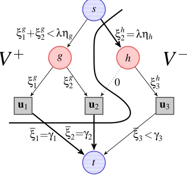
Let G be a directed graph G= (V,E,s,t), where V is a set of vertices, E_⊆V_×V a set of arcs, s

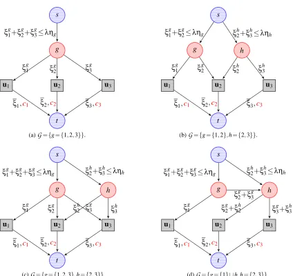
a source, and t a sink. For all arcs in E, we define a non-negative capacity constant, and as done classically in the network flow literature (Ahuja et al., 1993; Bertsekas, 1998), we define a flow as a non-negative function on arcs that satisfies capacity constraints on all arcs (the value of the flow on an arc is less than or equal to the arc capacity) and conservation constraints on all vertices (the sum of incoming flows at a vertex is equal to the sum of outgoing flows) except for the source and the sink. For every arc e in E, we also define a real-valued cost function, which depends on the value of the flow on e. We now introduce the canonical graph G associated with our optimization problem:

Definition 3 (Canonical Graph)

Let

G

⊆ {1, . . . ,p_} be a set of groups, and (ηg)g_∈G be positive weights. The canonical graph

G= (V,E,s,t)is the unique graph defined as follows:

1. V =Vu∪Vgr, where Vu is a vertex set of size p, one vertex being associated to each index j in {1, . . . ,p}, and Vgr is a vertex set of size |

G

|, one vertex per group g in

G

. We thus have_|V_|=_|

G

|+p. For simplicity, we identify groups g in

G

and indices j in_{1, . . . ,p_}with vertices of the graph, such that one can from now on refer to “vertex j” or “vertex g”.

2. For every group g in

G

, E contains an arc(s,g). These arcs have capacityληgand zero cost.

3. For every group g in

G

, and every index j in g, E contains an arc(g,j) with zero cost and infinite capacity. We denote byξg_j the flow on this arc.

4. For every index j in _{1, . . . ,p_}, E contains an arc (j,t) with infinite capacity and a cost

1

2(uj−ξj)2, whereξj is the flow on(j,t).

Examples of canonical graphs are given in Figures 1a-c for three simple group structures. The flowsξg_j associated with G can now be identified with the variables of problem (4). Since we have assumed the entries of u to be non-negative, we can now reformulate Equation (4) as

min ξ∈R₊p×|G|_,ξ∈Rp

p

∑

j=1

1

2(uj−ξj)

2 _{s.t. ξ=}

∑

g∈G

ξg

and ∀g∈

G

,

(

∑

j∈g

ξg

j ≤ληg and Supp(ξg)⊆g

)

.

(5) Indeed,

• the only arcs with a cost are those leading to the sink, which have the form(j,t), where j is the index of a variable in{1, . . . ,p}. The sum of these costs is∑p_j=11₂(uj−ξj)2, which is the

objective function minimized in Equation (5);

• by flow conservation, we necessarily haveξ_j=∑g∈Gξgj in the canonical graph;

• the only arcs with a capacity constraints are those coming out of the source, which have the form(s,g), where g is a group in

G

. By flow conservation, the flow on an arc(s,g)is∑j_∈gξgj

which should be less thanληgby capacity constraints;

Therefore we have shown that finding a flow minimizing the sum of the costs on such a graph is equivalent to solving problem (4). When some groups are included in others, the canonical graph can be simplified to yield a graph with a smaller number of edges. Specifically, if h and g are groups with h⊂g, the edges(g,j)for j∈h carrying a flowξg_j can be removed and replaced by a single edge

(g,h)of infinite capacity and zero cost, carrying the flow∑j∈hξ g

j. This simplification is illustrated

in Figure 1d, with a graph equivalent to the one of Figure 1c. This does not change the optimal value ofξ⋆, which is the quantity of interest for computing the optimal primal variable w⋆. We present in Appendix A a formal definition of equivalent graphs. These simplifications are useful in practice, since they reduce the number of edges in the graph and improve the speed of our algorithms.

3.4 Computation of the Proximal Operator

Quadratic min-cost flow problems have been well studied in the operations research literature (Hochbaum and Hong, 1995). One of the simplest cases, where

G

contains a single group as in Figure 1a, is solved by an orthogonal projection on theℓ1-ball of radiusληg. It has been shown,

both in machine learning (Duchi et al., 2008) and operations research (Hochbaum and Hong, 1995; Brucker, 1984), that such a projection can be computed in O(p)operations. When the group struc-ture is a tree as in Figure 1d, strategies developed in the two communities are also similar (Jenatton et al., 2010a; Hochbaum and Hong, 1995),8and solve the problem in O(pd)operations, where d is the depth of the tree.

The general case of overlapping groups is more difficult. Hochbaum and Hong (1995) have shown that quadratic min-cost flow problems can be reduced to a specific parametric max-flow problem, for which an efficient algorithm exists (Gallo et al., 1989).9 While this generic approach could be used to solve Equation (4), we propose to use Algorithm 1 that also exploits the fact that our graphs have non-zero costs only on edges leading to the sink. As shown in Appendix D, it it has a significantly better performance in practice. This algorithm clearly shares some similarities with existing approaches in network flow optimization such as the simplified version of Gallo et al. (1989) presented by Babenko and Goldberg (2006) that uses a divide and conquer strategy. Moreover, an equivalent algorithm exists for minimizing convex functions over polymatroid sets (Groenevelt, 1991). This equivalence, a priori non trivial, is uncovered through a representation of structured sparsity-inducing norms via submodular functions, which was recently proposed by Bach (2010).

The intuition behind our algorithm,computeFlow(see Algorithm 1), is the following: sinceξ= ∑g∈Gξgis the only value of interest to compute the solution of the proximal operator w=u−ξ, the

first step looks for a candidate valueγforξby solving the following relaxed version of problem (5):

arg min γ∈Rp _j

∑

∈Vu

1

2(uj−γj)

2 _s.t.

∑

j∈Vu

γ_j≤λ

∑

g∈Vgr

ηg. (6)

The cost function here is the same as in problem (5), but the constraints are weaker: Any feasible point of problem (5) is also feasible for problem (6). This problem can be solved in linear time (Brucker, 1984). Its solution, which we denoteγfor simplicity, provides the lower bound_ku₋γ_k2₂/2 for the optimal cost of problem (5).

8. Note however that, while Hochbaum and Hong (1995) only consider a tree-structured sum ofℓ∞-norms, the results from Jenatton et al. (2010a) also apply for a sum ofℓ2-norms.

s

g ξg

1+ξ

g

2+ξ

g

3≤ληg

u2 ξg 2 u1 ξg 1 u3 ξg 3 t

ξ1,c1 ξ2,c2 ξ₃,c3

(a)G={g={1,2,3}}.

s

g ξg

1+ξ

g

2≤ληg

h ξh

2+ξ

h

3≤ληh

u2 ξh 2 ξg 2 u1 ξg 1 u3 ξh 3 t

ξ1,c1 ξ2,c2 ξ₃,c3

(b)G={g={1,2},h={2,3}}.

s

g ξg

1+ξ

g

2+ξ

g

3≤ληg

h ξh

2+ξ

h

3≤ληh

u2 ξh 2 ξg 2 u1 ξg 1 u3 ξg

3 ξh₃

t

ξ₁,c1 ξ2,c2 ξ₃,c3

(c)G={g={1,2,3_},h={2,3_}}.

s

g ξg

1+ξ

g

2+ξ

g

3≤ληg

h ξh

2+ξ

h

3≤ληh

ξg

2+ξ

g

3

u2

ξg

2+ξ

h 2 u1 ξg 1 u3 ξg

3+ξ

h

3

t

ξ₁,c1 ξ2,c2 ξ₃,c3

(d)G={g={1_{} ∪}h,h={2,3_}}.

Figure 1: Graph representation of simple proximal problems with different group structures

G

. The three indices 1,2,3 are represented as grey squares, and the groups g,h in

G

as red (darker) discs. The source is linked to every group g,h with respective maximum capacityληg,ληhand zero cost.

Each variable uj is linked to the sink t, with an infinite capacity, and with a cost cj,1₂(uj−ξj)2.

Algorithm 1 Computation of the proximal operator for overlapping groups. input u_∈Rp_{, a set of groups}

_G

_{, positive weights(}η_g)g

∈G, andλ(regularization parameter).

1: Build the initial graph G0= (V0,E0,s,t)as explained in Section 3.4. 2: Compute the optimal flow:ξ_←computeFlow(V0,E0).

3: Return: w=u₋ξ(optimal solution of the proximal problem). FunctioncomputeFlow(V=Vu∪Vgr,E)

1: Projection step:γ_←arg min_γ∑j∈Vu 12(uj−γj)2 s.t. ∑j∈Vuγj≤λ∑g∈Vgrηg.

2: For all nodes j in Vu, setγjto be the capacity of the arc(j,t).

3: Max-flow step: Update(ξ_j)j_∈Vu by computing a max-flow on the graph(V,E,s,t).

4: if _∃ j_∈Vu s.t. ξj6=γjthen

5: Denote by(s,V+_)and(V−_{,t)the two disjoint subsets of(V,s,t)separated by the minimum}

(s,t)-cut of the graph, and remove the arcs between V+ and V−. Call E+ and E− the two remaining disjoint subsets of E corresponding to V+and V−.

6: (ξ_j)_j∈V+

u ←computeFlow(V +_,E+_).

7: (ξ_j)_j∈V−

u ←computeFlow(V

−_,E−_). 8: end if

9: Return:(ξ_j)j∈Vu.

The second step tries to construct a feasible flow(ξ,ξ), satisfying additional capacity constraints equal toγj on arc(j,t), and whose cost matches this lower bound; this latter problem can be cast

as a max-flow problem (Goldberg and Tarjan, 1986). If such a flow exists, the algorithm returns

ξ=γ, the cost of the flow reaches the lower bound, and is therefore optimal. If such a flow does not exist, we haveξ₆=γ, the lower bound is not achievable, and we build a minimum(s,t)-cut of the graph (Ford and Fulkerson, 1956) defining two disjoints sets of nodes V+ and V−; V+ is the part of the graph which is reachable from the source (for every node j in V+, there exists a non-saturated path from s to j), whereas all paths going from s to nodes in V−are saturated. More details about these properties can be found at the beginning of Appendix B. At this point, it is possible to show that the value of the optimal min-cost flow on all arcs between V+and V− is necessary zero. Thus, removing them yields an equivalent optimization problem, which can be decomposed into two independent problems of smaller sizes and solved recursively by the calls tocomputeFlow(V+,E+₎ andcomputeFlow(V−,E−). A formal proof of correctness of Algorithm 1 and further details are relegated to Appendix B.

The approach of Hochbaum and Hong (1995); Gallo et al. (1989) which recasts the quadratic min-cost flow problem as a parametric max-flow is guaranteed to have the same worst-case com-plexity as a single max-flow algorithm. However, we have experimentally observed a significant discrepancy between the worst case and empirical complexities for these flow problems, essentially because the empirical cost of each max-flow is significantly smaller than its theoretical cost. Despite the fact that the worst-case guarantees for our algorithm is weaker than theirs (up to a factor_|V_|), it is more adapted to the structure of our graphs and has proven to be much faster in our experiments (see Appendix D).10 Some implementation details are also crucial to the efficiency of the algorithm: 10. The best theoretical worst-case complexity of a max-flow is achieved by Goldberg and Tarjan (1986) and is

O |V||E|log(|V|2_/|E|)

• Exploiting maximal connected components: When there exists no arc between two sub-sets of V , the solution can be obtained by solving two smaller optimization problems cor-responding to the two disjoint subgraphs. It is indeed possible to process them indepen-dently to solve the global min-cost flow problem. To that effect, before calling the function

computeFlow(V,E), we look for maximal connected components(V1,E1), . . . ,(VN,EN)and

call sequentially the procedurecomputeFlow(Vi,Ei) for i in{1, . . . ,N}.

• Efficient max-flow algorithm: We have implemented the “push-relabel” algorithm of Gold-berg and Tarjan (1986) to solve our max-flow problems, using classical heuristics that signif-icantly speed it up in practice; see Goldberg and Tarjan (1986) and Cherkassky and Goldberg (1997). We use the so-called “highest-active vertex selection rule, global and gap heuris-tics” (Goldberg and Tarjan, 1986; Cherkassky and Goldberg, 1997), which has a worst-case complexity of O(_|V_|2_|E_|1/2)for a graph(V,E,s,t). This algorithm leverages the concept of

pre-flow that relaxes the definition of flow and allows vertices to have a positive excess.

• Using flow warm-restarts: The max-flow steps in our algorithm can be initialized with any valid pre-flow, enabling warm-restarts. This is also a key concept in the parametric max-flow algorithm of Gallo et al. (1989).

• Improved projection step: The first line of the procedurecomputeFlowcan be replaced by

γ_←arg min_γ∑j∈Vu12(uj−γj)2 s.t. ∑j∈Vuγj≤λ∑g∈Vgrηg and|γj| ≤λ∑g∋jηg.The idea is

to build a relaxation of Equation (5) which is closer to the original problem than the one of Equation (6), but that still can be solved in linear time. The structure of the graph will indeed not allowξ_j to be greater thanλ∑g∋jηg after the max-flow step. This modified projection

step can still be computed in linear time (Brucker, 1984), and leads to better performance.

3.5 Computation of the Dual Norm

The dual normΩ∗ofΩ, defined for any vectorκinRp_by

Ω∗_{(κ), max} Ω(z)≤1z

⊤_κ,

is a key quantity to study sparsity-inducing regularizations in many respects. For instance, dual norms are central in working-set algorithms (Jenatton et al., 2009; Bach et al., 2011), and arise as well when proving theoretical estimation or prediction guarantees (Negahban et al., 2009).

In our context, we use it to monitor the convergence of the proximal method through a duality gap, hence defining a proper optimality criterion for problem (1). As a brief reminder, the duality gap of a minimization problem is defined as the difference between the primal and dual objective functions, evaluated for a feasible pair of primal/dual variables (see Section 5.5, Boyd and Vanden-berghe, 2004). This gap serves as a certificate of (sub)optimality: if it is equal to zero, then the optimum is reached, and provided that strong duality holds, the converse is true as well (see Sec-tion 5.5, Boyd and Vandenberghe, 2004). A descripSec-tion of the algorithm we use in the experiments (Beck and Teboulle, 2009) along with the integration of the computation of the duality gap is given in Appendix C.

We now denote by f∗ the Fenchel conjugate of f (Borwein and Lewis, 2006), defined by

f∗(κ),sup_z[z⊤κ₋f(z)]. The duality gap for problem (1) can be derived from standard Fenchel duality arguments (Borwein and Lewis, 2006) and it is equal to

f(w) +λΩ(w) +f∗(₋κ)for w,κinRp_withΩ∗₍κ_)≤λ_.

Therefore, evaluating the duality gap requires to compute efficientlyΩ∗in order to find a feasible dual variableκ(the gap is otherwise equal to+∞and becomes non-informative). This is equivalent to solving another network flow problem, based on the following variational formulation:

Ω∗_{(κ) = min}

ξ∈Rp×|G|τ s.t.

∑

g∈G

ξg

=κ,and_∀g_∈

G

,_kξg_k1≤τηg with ξgj =0 if j∈/g. (7)

In the network problem associated with (7), the capacities on the arcs(s,g), g∈

G

, are set toτηg,

and the capacities on the arcs(j,t), j in_{1, . . . ,p_}, are fixed toκj. Solving problem (7) amounts

to finding the smallest value ofτ, such that there exists a flow saturating all the capacitiesκj on the

arcs leading to the sink t. Equation (7) and Algorithm 2 are proven to be correct in Appendix B.

Algorithm 2 Computation of the dual norm.

input κ_∈Rp_{, a set of groups}

_G

_{, positive weights(}η_g)g

∈G.

1: Build the initial graph G0= (V0,E0,s,t)as explained in Section 3.5. 2: τ←dualNorm(V0,E0).

3: Return:τ(value of the dual norm). FunctiondualNorm(V=Vu∪Vgr,E)

1: τ←(∑_j∈Vuκ_j)/(∑_g∈Vgrη_g)and set the capacities of arcs(s,g)toτηgfor all g in Vgr.

2: Max-flow step: Update(ξ_j)j∈Vu by computing a max-flow on the graph(V,E,s,t).

3: if _∃ j_∈Vu s.t. ξj6=κj then

4: Define(V+,E+)and(V−,E−)as in Algorithm 1, and setτ_←dualNorm(V−,E−). 5: end if

6: Return: τ.

4. Optimization with Proximal Splitting Methods

We now present proximal splitting algorithms (see Combettes and Pesquet, 2008, 2010; Tomioka et al., 2011; Boyd et al., 2011, and references therein) for solving Equation (1). Differentiability of f is not required here and the regularization function can either be a sum of ℓ2- orℓ∞-norms. However, we assume that:

(A) either f can be written f(w) =∑n

i=1f˜i(w), where the functions ˜fiare such that prox_γfi˜ can be obtained in closed form for allγ>0 and all i—that is, for all u inRm_{, the following problems}

admit closed form solutions: minv∈Rm1

2ku−vk 2

2+γf˜i(v).

(B) or f can be written f(w) = f˜(Xw)for all w inRp_{, where X in}Rn×p _{is a design matrix, and}

It is easy to show that this condition is satisfied for the square and hinge loss functions, making it possible to build linear SVMs with a structured sparse regularization. These assumptions are not the same as the ones of Section 3, and the scope of the problems addressed is therefore slightly dif-ferent. Proximal splitting methods seem indeed to offer more flexibility regarding the regularization function, since they can deal with sums of ℓ2-norms.11 However, proximal gradient methods, as presented in Section 3, enjoy a few advantages over proximal splitting methods, namely: automatic parameter tuning with line-search schemes (Nesterov, 2007), known convergence rates (Nesterov, 2007; Beck and Teboulle, 2009), and ability to provide sparse solutions (approximate solutions obtained with proximal splitting methods often have small values, but not “true” zeros).

4.1 Algorithms

We consider a class of algorithms which leverage the concept of variable splitting (see Combettes and Pesquet, 2010; Bertsekas and Tsitsiklis, 1989; Tomioka et al., 2011). The key is to introduce additional variables zginR|g|_{, one for every group g in}

_G

_{, and equivalently reformulate Equation (1)}

as

min

w_∈Rp

zg

∈R|g|_{for g∈G}

f(w) +λ

∑

g_∈G

ηgkzgk s.t. ∀g∈

G

, zg=wg, (8)

The issue of overlapping groups is removed, but new constraints are added, and as in Section 3, the method introduces additional variables which induce a memory cost of O(∑g∈G|g|).

To solve this problem, it is possible to use the so-called alternating direction method of multi-pliers (ADMM) (see Combettes and Pesquet, 2010; Bertsekas and Tsitsiklis, 1989; Tomioka et al., 2011; Boyd et al., 2011).12 It introduces dual variables νg in R|g| _{for all g in}

_G

_{, and defines the}

augmented Lagrangian:

L

w,(zg)g∈G,(νg)g∈G,f(w) +

∑

g_∈G

λη

gkzgk+νg⊤(zg−wg) +

γ

2kz

g_−w gk22

,

whereγ>0 is a parameter. It is easy to show that solving Equation (8) amounts to finding a saddle-point of the augmented Lagrangian.13 The ADMM algorithm finds such a saddle-point by iterating between the minimization of

L

with respect to each primal variable, keeping the other ones fixed, and gradient ascent steps with respect to the dual variables. More precisely, it can be summarized as:

1. Minimize

L

with respect to w, keeping the other variables fixed.

11. We are not aware of any efficient algorithm providing the exact solution of the proximal operator associated to a sum ofℓ2-norms, which would be necessary for using (accelerated) proximal gradient methods. An iterative algorithm could possibly be used to compute it approximately (e.g., see Jenatton et al., 2010a, 2011), but such a procedure would be computationally expensive and would require to be able to deal with approximate computations of the proximal operators (e.g., see Combettes and Pesquet, 2010; Schmidt et al., 2011, and discussions therein). We have chosen not to consider this possibility in this paper.

12. This method is used by Sprechmann et al. (2010) for computing the proximal operator associated to hierarchical norms, and independently in the same context as ours by Boyd et al. (2011) and Qin and Goldfarb (2011).

13. The augmented Lagrangian is in fact the classical Lagrangian (see Boyd and Vandenberghe, 2004) of the following optimization problem which is equivalent to Equation (8):

min w∈Rp_,(zg_∈R|g|)g∈G

f(w) +λ

∑

g∈G

ηgkzgk+γ

2kz

g

2. Minimize

L

with respect to the zg’s, keeping the other variables fixed. The solution can be obtained in closed form: for all g in

G

, zg_←proxληg

γ k.k[wg−

1 γνg].

3. Take a gradient ascent step on

L

with respect to theνg’s: νg_←νg+γ(zg₋wg).

4. Go back to step 1.

Such a procedure is guaranteed to converge to the desired solution for all value ofγ>0 (however, tuningγcan greatly influence the convergence speed), but solving efficiently step 1 can be difficult. To cope with this issue, we propose two variations exploiting assumptions (A) and (B).

4.1.1 SPLITTING THELOSSFUNCTION f

We assume condition (A)—that is, we have f(w) =∑n_i=1f˜i(w). For example, when f is the square

loss function f(w) = 1

2ky−Xwk 2

2, where X inRn×p is a design matrix and y is inRn, we would define for all i in_{1, . . . ,n_}the functions ˜fi:R→Rsuch that ˜fi(w),1₂(yi−x⊤i w)2, where xi is

the i-th row of X.

We now introduce new variables vi inRp_{for i=1, . . . ,n, and replace f(w)in Equation (8) by} ∑n

i=1f˜i(vi), with the additional constraints that vi=w. The resulting equivalent optimization

prob-lem can now be tackled using the ADMM algorithm, following the same methodology presented above. It is easy to show that every step can be obtained efficiently, as long as one knows how to compute the proximal operator associated to the functions ˜fiin closed form. This is in fact the case

for the square and hinge loss functions, where n is the number of training points. The main problem of this strategy is the possible high memory usage it requires when n is large.

4.1.2 DEALING WITH THEDESIGNMATRIX

If we assume condition (B), another possibility consists of introducing a new variable v in Rn_,

such that one can replace the function f(w) = f˜(Xw)by ˜f(v)in Equation (8) with the additional constraint v=Xw. Using directly the ADMM algorithm to solve the corresponding problem implies adding a termκ⊤(v₋Xw) +₂γ_kv₋Xw_k2₂to the augmented Lagrangian

L

, whereκis a new dual variable. The minimization of

L

with respect to v is now obtained by v_←prox1

γf˜[Xw−κ], which

is easy to compute according to (B). However, the design matrix X in the quadratic term makes the minimization of

L

with respect to w more difficult. To overcome this issue, we adopt a strategy presented by Zhang et al. (2011), which replaces at iteration k the quadratic term γ_2kv₋Xw_k2

2in the augmented Lagrangian by an additional proximity term: ₂γ_kv₋Xw_k2₂+₂γ_kw₋wk_k2_Q, where wk is the current estimate of w, and_kw₋wk_k2_Q= (w₋wk)⊤Q(w₋wk), where Q is a symmetric positive definite matrix. By choosing Q,δI₋X⊤X, withδlarge enough, minimizing

L

with respect to w becomes simple, while convergence to the solution is still ensured. More details can be found in Zhang et al. (2011).

5. Applications and Experiments

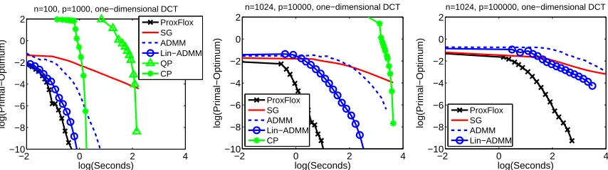
5.1 Speed Benchmark

We consider a structured sparse decomposition problem with overlapping groups ofℓ_∞-norms, and compare the proximal gradient algorithm FISTA (Beck and Teboulle, 2009) with our proximal op-erator presented in Section 3 (referred to as ProxFlow), two variants of proximal splitting methods, (ADMM) and (Lin-ADMM) respectively presented in Section 4.1.1 and 4.1.2, and two generic optimization techniques, namely a subgradient descent (SG) and an interior point method,14 on a regularized linear regression problem. SG, ProxFlow, ADMM and Lin-ADMM are implemented inC++.15 _{Experiments are run on a single-core 2.8 GHz CPU. We consider a design matrix X in}

Rn×p_{built from overcomplete dictionaries of discrete cosine transforms (DCT), which are naturally}

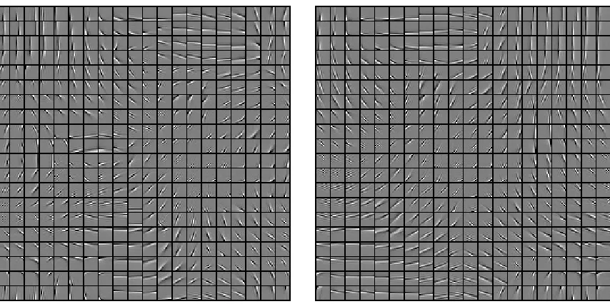
organized on one- or two-dimensional grids and display local correlations. The following families of groups

G

using this spatial information are thus considered: (1) every contiguous sequence of length 3 for the one-dimensional case, and (2) every 3_×3-square in the two-dimensional setting. We generate vectors y inRn_{according to the linear model y=Xw0+}ε_{, where}ε_∼

_N

_(0,0.01kXw0k2

2). The vector w0has about 20% percent nonzero components, randomly selected, while respecting the structure of

G

, and uniformly generated in[₋1,1].

In our experiments, the regularization parameterλis chosen to achieve the same level of spar-sity (20%). For SG, ADMM and Lin-ADMM, some parameters are optimized to provide the low-est value of the objective function after 1 000 iterations of the respective algorithms. For SG, we take the step size to be equal to a/(k+b), where k is the iteration number, and (a,b) are the pair of parameters selected in _{10−3, . . . ,10_}×{102,103,104_}. Note that a step size of the form a/(√t+b) is also commonly used in subgradient descent algorithms. In the context of hi-erarchical norms, both choices have led to similar results (Jenatton et al., 2011). The parameterγ for ADMM is selected in _{10−2, . . . ,102_}. The parameters (γ,δ) for Lin-ADMM are selected in {10−2, . . . ,102_{} × {}10−1, . . . ,108_}. For interior point methods, since problem (1) can be cast either as a quadratic (QP) or as a conic program (CP), we show in Figure 2 the results for both formu-lations. On three problems of different sizes, with(n,p)_{∈ {}(100,103),(1024,104),(1024,105)_}, our algorithms ProxFlow, ADMM and Lin-ADMM compare favorably with the other methods, (see Figure 2), except for ADMM in the large-scale setting which yields an objective function value similar to that of SG after 104 seconds. Among ProxFlow, ADMM and Lin-ADMM, ProxFlow is consistently better than Lin-ADMM, which is itself better than ADMM. Note that for the small scale problem, the performance of ProxFlow and Lin-ADMM is similar. In addition, note that QP, CP, SG, ADMM and Lin-ADMM do not obtain sparse solutions, whereas ProxFlow does.16 5.2 Wavelet Denoising with Structured Sparsity

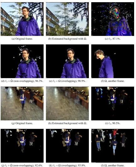
We now illustrate the results of Section 3, where a single large-scale proximal operator (p_≈250 000) associated to a sum of ℓ_∞-norms has to be computed. We choose an image denoising task with an orthonormal wavelet basis, following an experiment similar to one proposed in Jenatton et al. (2011). Specifically, we consider the following formulation

min

w∈Rp

1

2ky−Xwk 2

2+λΩ(w),

14. In our simulations, we use the commercial softwareMosek,http://www.mosek.com/

15. Our implementation of ProxFlow is available athttp://www.di.ens.fr/willow/SPAMS/.

−2 0 2 4 −10 −8 −6 −4 −2 0 2

n=100, p=1000, one−dimensional DCT

log(Seconds) log(Primal−Optimum) ProxFlox SG ADMM Lin−ADMM QP CP

−2 0 2 4

−10 −8 −6 −4 −2 0 2

n=1024, p=10000, one−dimensional DCT

log(Seconds) log(Primal−Optimum) ProxFlox SG ADMM Lin−ADMM CP

−2 0 2 4

−10 −8 −6 −4 −2 0 2

n=1024, p=100000, one−dimensional DCT

log(Seconds) log(Primal−Optimum) ProxFlox SG ADMM Lin−ADMM

Figure 2: Speed comparisons: distance to the optimal primal value versus CPU time (log-log scale). Due to the computational burden, QP and CP could not be run on every problem.

where y inRp_{is a noisy input image, w represents wavelets coefficients, X in}Rp×p_{is an}

orthonor-mal wavelet basis, Xw is the estimate of the denoised image, andΩis a sparsity-inducing norm. Since here the basis is orthonormal, solving the decomposition problem boils down to computing w⋆=prox_λΩ[X⊤y]. This makes of Algorithm 1 a good candidate to solve it whenΩis a sum of

ℓ∞-norms. We compare the following candidates for the sparsity-inducing normsΩ:

• theℓ1-norm, leading to the wavelet soft-thresholding of Donoho and Johnstone (1995). • a sum ofℓ∞-norms with a hierarchical group structure adapted to the wavelet coefficients, as

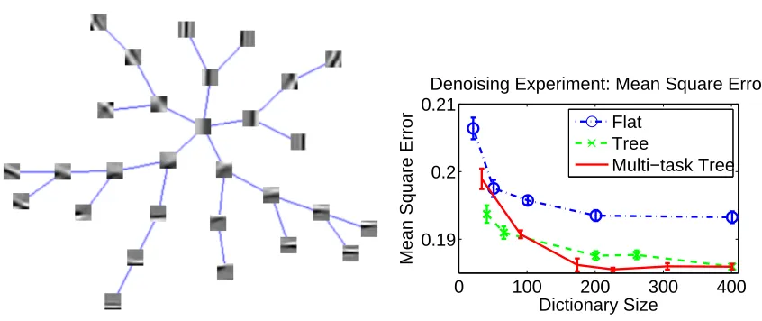
proposed in Jenatton et al. (2011). Considering a natural quad-tree for wavelet coefficients (see Mallat, 1999), this norm takes the form of Equation (2) with one group per wavelet coefficient that contains the coefficient and all its descendants in the tree. We call this norm

Ωtree.

• a sum ofℓ_∞-norms with overlapping groups representing 2_×2 spatial neighborhoods in the wavelet domain. This regularization encourages neighboring wavelet coefficients to be set to zero together, which was also exploited in the past in block-thresholding approaches for wavelet denoising (Cai, 1999). We call this normΩgrid.

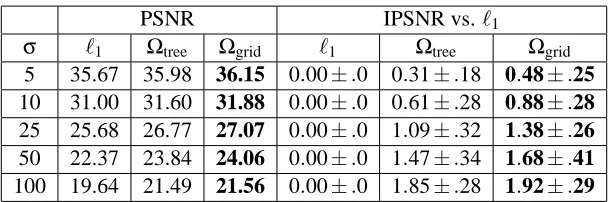
We consider Daubechies3 wavelets (see Mallat, 1999) for the matrix X, use 12 classical standard test images,17 and generate noisy versions of them corrupted by a white Gaussian noise of vari-ance σ2_{. For each image, we test several values of} λ₌₂₄iσ√_{log p, with i taken in the range} {−15,₋14, . . . ,15_}. We then keep the parameterλgiving the best reconstruction error on average on the 12 images. The factorσ√log p is a classical heuristic for choosing a reasonable regulariza-tion parameter (see Mallat, 1999). We provide reconstrucregulariza-tion results in terms of PSNR in Table 1.18 Unlike Jenatton et al. (2011), who set all the weights ηg inΩequal to one, we tried exponential

weights of the formηg=ρk, with k being the depth of the group in the wavelet tree, andρis taken

in_{0.25,0.5,1,2,4_}. As forλ, the value providing the best reconstruction is kept. The wavelet transforms in our experiments are computed with the matlabPyrTools software.19 Interestingly, we observe in Table 1 that the results obtained withΩgrid are significantly better than those obtained 17. These images are used in classical image denoising benchmarks. See Mairal et al. (2009).

PSNR IPSNR vs.ℓ1

σ ℓ1 Ωtree Ωgrid ℓ1 Ωtree Ωgrid

5 35.67 35.98 36.15 0.00_±.0 0.31_±.18 0.48_±.25 10 31.00 31.60 31.88 0.00_±.0 0.61_±.28 0.88_±.28 25 25.68 26.77 27.07 0.00_±.0 1.09_±.32 1.38_±.26 50 22.37 23.84 24.06 0.00±.0 1.47±.34 1.68±.41 100 19.64 21.49 21.56 0.00_±.0 1.85_±.28 1.92_±.29

Table 1: PSNR measured for the denoising of 12 standard images when the regularization function is theℓ1-norm, the tree-structured norm Ωtree, and the structured normΩgrid, and improvement in PSNR compared to theℓ1-norm (IPSNR). Best results for each level of noise and each wavelet type are in bold. The reported values are averaged over 5 runs with different noise realizations.

withΩtree, meaning that encouraging spatial consistency in wavelet coefficients is more effective than using a hierarchical coding. We also note that our approach is relatively fast, despite the high dimension of the problem. Solving exactly the proximal problem with Ωgrid for an image with

p=512_×512=262 144 pixels (and therefore approximately the same number of groups) takes approximately_≈4₋6 seconds on a single core of a 3.07GHz CPU.

5.3 CUR-like Matrix Factorization

In this experiment, we show how our tools can be used to perform the so-called CUR matrix decom-position (Mahoney and Drineas, 2009). It consists of a low-rank approximation of a data matrix X inRn×p_{in the form of a product of three matrices—that is, X≈CUR. The particularity of the CUR}

decomposition lies in the fact that the matrices C_∈Rn×c_{and R∈}Rr×p_{are constrained to be}

respec-tively a subset of c columns and r rows of the original matrix X. The third matrix U_∈Rc×r_{is then}

given by C+XR+, where A+ denotes a Moore-Penrose generalized inverse of the matrix A (Horn and Johnson, 1990). Such a matrix factorization is particularly appealing when the interpretability of the results matters (Mahoney and Drineas, 2009). For instance, when studying gene-expression data sets, it is easier to gain insight from the selection of actual patients and genes, rather than from linear combinations of them.

In Mahoney and Drineas (2009), CUR decompositions are computed by a sampling procedure based on the singular value decomposition of X. In a recent work, Bien et al. (2010) have shown that

partial CUR decompositions, that is, the selection of either rows or columns of X, can be obtained

by solving a convex program with a group-Lasso penalty. We propose to extend this approach to the simultaneous selection of both rows and columns of X, with the following convex problem:

min

W∈Rp×n

1

2kX−XWXk 2 F+λrow

n

∑

i=1

kWi_k∞+λcol

p

∑

j=1

kWjk∞. (9)

In this formulation, the two sparsity-inducing penalties controlled by the parametersλrow andλcol set to zero some entire rows and columns of the solutions of problem (9). Now, let us denote by WI J inR|I|×|J| _{the submatrix of W reduced to its nonzero rows and columns, respectively indexed by}

I_{⊆ {}1, . . . ,p_}and J_{⊆ {}1, . . . ,n_}. We can then readily identify the three components of the CUR decomposition of X, namely