Vol. 15, No. 2, 2018, 157-166
ISSN: 2320 –3242 (P), 2320 –3250 (online) Published on 30 April 2018
www.researchmathsci.org
DOI: http://dx.doi.org/10.22457/ijfma.v15n2a6
157
International Journal of
Modelling and Analysis of Compliment Inventory System
in Supply Chain with Partial Backlogging
B. Amala Jasmine1 and K. Krishnan2 1
PG & Research Department of Mathematics, Jeyaraj Annapackiam College for Women Periyakulam Tamil Nadu, India -625513
Email: [email protected] 2
PG & Research Department of Mathematics, Cardamom Planters’ Association College Bodinayakanur, Tamil Nadu, India -625513
2
Corresponding author. Email: [email protected] Received 17 March 2018; accepted 21 April 2018
Abstract. This paper presents a continuous review two echelon inventory systems with
two different items in stock, one is main product and other one is complement item for the main product. The operating policy at the lower echelon for the main product is (s, S) that is whenever the inventory level drops to ‘s’ on order for Q = (S-s) items is placed, the ordered items are received after a random time which is distributed as exponential. We assume that the demands accruing during the stock-out period are partially backlogged. The retailer replenishes the stock of main product from the supplier which adopts (0,M) policy. The complement product is replenished instantaneously from local supplier. The joint probability disruption of the inventory levels of main product, complement item at retailer and the main product at supplier are obtained in the steady state case. Various system performance measures are derived and the long run total expected inventory cost rate is calculated. Several instances of numerical examples, which provide insight into the behavior of the system, are presented.
Keywords: Continuous review inventory system, Two-echelon, Positive lead time, Lost
sale.
AMS Mathematics Subject Classification (2010): 90B05
1. Introduction
158
The main objective for a multi-echelon inventory model is to coordinate the inventories at the various echelons so as to minimize the total cost associated with the entire multi-echelon inventory system. This is a natural objective for a fully integrated corporation that operates the entire system. It might also be a suitable objective when certain echelons are managed by either the suppliers or the retailers of the company. Multi-echelon inventory system has been studied by many researchers and its applications in supply chain management has proved worthy in recent literature.
As supply chains integrates many operators in the network and optimize the total cost involved without compromising as customer service efficiency. The first quantitative analysis in inventory studies Started with the work of Harris [9]. Clark and Scarf [7] had put forward the multi-echelon inventory first. They analyzed a N-echelon pipelining system without considering a lot size. One of the oldest papers in the field of continuous review multi-echelon inventory system is written by Sherbrooke in 1968. Hadley and Whitin [6], Naddor [14] analyses various inventory Systems. HP's (Hawlett Packard) Strategic Planning and Modeling (SPaM) group initiated this kind of research in 1977.
Sivazlian and Stanfel [16] analyzed a two commodity single period inventory system. Kalpakam and Arivarignan [10] analyzed a multi-item inventory model with renewal demands under a joint replenishment policy. They assumed instantaneous supply of items and obtain various operational characteristics and also an expression for the long run total expected cost rate. Krishnamoorthy et al., [11] analyzed a two commodity continuous review inventory system with zero lead time. A two commodity problem with Markov shift in demand for the type of commodity required, is considered by Krishnamoorthy and Varghese [12]. They obtain a characterization for limiting probability distribution to be uniform. Associated optimization problems were discussed in all these cases. However in all these cases zero lead time is assumed.
In the literature of stochastic inventory models, there are two different assumptions about the excess demand unfilled from existing inventories: the backlog assumption and the lost sales assumption. The former is more popular in the literature partly because historically the inventory studies started with spare parts inventory management problems in military applications, where the backlog assumption is realistic. However in many other business situations, it is quite often that demand that cannot be satisfied on time is lost. This is particularly true in a competitive business environment. For example in many retail establishments, such as a supermarket or a department store, a customer chooses a competitive brand or goes to another store if his/her preferred brand is out of stock.
All these papers deal with repairable items with batch ordering. A complete review was provided by Beamon [5]. Axsater [1] proposed an approximate model of inventory structure in SC. He assumed (S-1, S) polices in the Deport-Base systems for repairable items in the American Air Force and could approximate the average inventory and stock out level in bases.
Anbazhagan and Arivarignan [2,3] have analyzed two commodity inventory system under various ordering policies. Yadavalli et al., [19] have analyzed a model with joint ordering policy and varying order quantities. Yadavalli et al., [20] have considered a two commodity substitutable inventory system with Poisson demands and arbitrarily distributed lead time.
Backlogging
159
major item, with random lead time but instantaneous replenishment for the gift item are considered. The lost sales for major item is also assumed when the items are out of stock. The above model is studied only at single location (Lower echelon). We extend the same in to multi-echelon structure (Supply Chain). The rest of the paper is organized as follows. The model formulation is described in section 2, along with some important notations used in the paper. In section 3, steady state analysis are done: Section 4 deals with the derivation of operating characteristics of the system. In section 5, the cost analysis for the operation. Section 6 provides Numerical examples and sensitivity analysis.
2. Model
2.1. The problem description
The inventory control system considered in this paper is defined as follows. A finished main product is supplied from manufacturer to supplier which adopts (0,M) replenishment policy then the product is supplied to retailer who adopts (s,S) policy. The retailer also maintain inventory of the complement product which has instantaneous replenishment from local supplier. The demand at retailer node follows an independent Poisson distribution with rate (i = 1, 2) for main product and complement respectively. Demands accruing during the stock out periods of main product are backlogged up to some finite number b. The replacement of item in terms of product is made from supplier to retailer is administrated with exponential distribution having parameter
µ
>0. The maximum inventory level at retailer node for main product is S, and the recorder point is s and the ordering quantity is Q ( = S-s) items. The maximum inventory at supplier in M( = nQ) .2.2. Notations and variables
We use the following notations and variables for the analysis of the paper. Notations
/variables
Used for
[ ]
C ijThe element of sub matrix at (i,j)th position of C
0 Zero matrix
, Mean arrival rate for Main& Compliment product at retailer
µ
Mean replacement rate for main product at retailerS, N Minimum inventory level for main& Compliment product at retailer s reorder level for main product at retailer
b Backlog capacity
M Maximum inventory level for main product at supplier Hm Holding cost per item for main product at retailer
160 O
m Ordering cost per order for main product at retailer Im Average inventory level for main product at retailer Ic Average inventory level for compliment product at retailer Id Average inventory level for main product at retailer
Rd Mean reorder rate for main product at supplier. Rc Mean reorder rate for compliment product at retailer
Rm Mean reorder rate for main product at retailer Sm Shortage rate for main product at retailer Tm Penalty rate for main product at retailer
=
∑
nQi Q
i Q + 2Q + 3Q + ... + nQ
3. Analysis
Let and denote the on hand Inventory levels of Main product, Compliment product at retailer and denote the on hand inventory level of Main product at supplier at time t+.
We define I (t) = as Markov process with
state space E = { ( i, j, k) | i = S, S-1, ...s,..1, 0, -1, -2, ...-b, j =1, 2, …, N, k=Q,2Q,...nQ }. Since E is finite and all its states are aperiodic, recurrent, non- null and also irreducible. That is all the states are Ergodic. Hence the limiting distribution exists and is independent of the initial state.
The infinitesimal generator matrix of this process C = ( a ( i, j, k, :l, m, n))( , , )( , , )i j k l m n∈E can be obtained from the following arguments.
• The arrival of a demand for main product at retailer make a state transition in the Markov process from (i, j, k ) to ( i-1, j-1, k ) with the intensity of transition
λ
1> 0.• The arrival of a demand for compliment product at retailer make a state transition in the Markov process from (i, j, k ) to ( i, j-1, k ) with the intensity of transition
2
λ
> 0.• The replacement of inventory at retailer make a state transition in the Markov process from (i, j, k ) to ( i+Q, j, k-Q ) or (i, j, Q ) to ( i+Q, j, nQ ) with the intensity of transition µ> 0.
The infinitesimal generator C is given by
C=
0 .... 0 0
0 .... 0 0
....
0 0 0 ....
0 0 .... 0
A B A B
A B
B A
⋮ ⋮ ⋮ ⋮ ⋮
Backlogging
161
[ ]
C pq=; , ( 1) ,...
; ( 1) ,....
( 1)
0
A p q q nQ n Q Q B p q Q q n Q Q
B p q n Q q nQ otherwise
= = −
= + = −
= − − =
Where the entries of the matrices are given by
[ ]
Aij= 12
2
; 1, 2,...
1 ; 1, 2,...( 1)
( 1) ;
0
= =
+ = = −
− − = =
A i j i N A i j i N A i N j i N
otherwise
[ ]
Bij=1 ;i 1, 2,...,
0
= =
B i j N otherwise
The elements in the sub matrices of A and B are
0 otherwise
0 otherwise
0 otherwise
3.1. Steady state analysis
The structure of the infinitesimal matrix C, reveals that the state space E of the Markov process {I (t) : t ≥ 0 } is finite and irreducible. Let the limiting probability distribution of
the inventory level process be
where the steady state probability that the system be in state (i, j, k).
Let denote the steady state probability distribution.
162
(i)
∏
nQj A1+∏
inQA2+∏
Qj B1=0 i = 1; j = S(ii) nQ 1 (n 1)Q 1 (n 1)Q 2
j B j A i A 0
− −
+ + =
∏
∏
∏
i = 1; j = S(iii) (n 1)Q 1 Q 1 Q 2
j B j A i A 0
−
+ + =
∏
∏
∏
i = 1; j = S(iv)
∏
nQj A2+∏
i 1nQ− A1+∏
i 1Q− B1=0 i = S, S-1,…….,2,1,0,-1,-2…-(b+2)(v) nQi 1B1 (n 1)Qi A2 ( n 1)Qi 1 A1 0
− −
− + + − =
∏
∏
∏
i = S, S-1,…….,2,1,0,-1,-2…-(b+2)(vi) ( n 1)Q 1 Q 2 Q 1
i 1 B i A i 1A 0
−
− + + − =
∏
∏
∏
i = S, S-1,…….,2,1,0,-1,-2…-(b+2)By solving the above system of equations, together with normalizing
condition
( , , ) ,
1
∈
=
∏
∑
i j k k
j
E i
, the steady probability of all the system states are obtained.
4. Operating characteristic
In this section we derive some important system performance measures.
4.1. Average inventory level
The event Im, Ic and Id denote the average inventory level for main product, complement
product at retailer and main product at distributor respectively,
4.2. Mean reorder rate
Let Rm , Rc , and Rd be the mean reorder rate for main product, complement product at
retailer and main product at distributor respectively,
4.3. Shortage rate
Shortage occur at retailer only for main product. Let Sm be the shortage rate at retailer for
main product, then
(i) = 1
1 b,
= = −
∑ ∑
nQ N∏
k Q j k
j
Backlogging
163 5. Cost analysis
In this section we impose a cost structure for the proposed model and analyze it by the criteria of minimization of long run total expected cost per unit time. The long run expected cost rate TC(s, Q)is given by
TC(s, Q)= Im.Hm + Ic.Hc + Id.Hd + Rm. Om + Rc.Oc + Rd.Od + Sm. Tm
Although we have a not proved analytically the convexity of the cost function TC(s, Q) our experience with considerable numberof numerical examples indicate that TC(s, Q) for fixed ‘S’ appears to be convex in s. In some cases it turned out to be increasing function of s. For large number case of TC(s, Q)revealed a locally convex structure. Hence we adopted the numerical search procedure to determine the optimal value of ‘s’
6. Numerical example and sensitivity analysis 6.1. Numerical example
In this section we discuss the problem of minimizing the structure. We assume Hc≤ Hm≤ Hd, i.e, the holding cost for compliment product is at retailer node is less than that of main product at retailer node and the holding cost of main product is less than that of main product at distributor node. Also Oc≤ Om≤Od the ordering cost at retailer node for compliment product is less than that of main product. Also the ordering cost at the distributor is greater than that of compliment product at retailer node.
The results we obtained in the steady state case may be illustrated through the following numerical example,
S = 16, N = 15, M = 80,
λ
1 =3,λ
2 =2, b = 3µ
=3, Hc=1.1, Hm =1.2, Hd =1.3
2.1, 2.2, 2.3
= = =
c m d
O O O Tm =3.1
The cost for different reorder level are given by
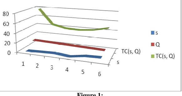
S 1 2 3 4* 5 6
Q 15 14 13 12 11 10
TC(s, Q) 77.98279 45.35418 38.8074 37.67178 40.40994 47.31084 Table 1: Total expected cost rate as a function s and Q
For the inventory capacity S, the optimal reorder level s* and optimal cost TC(s, Q)are indicated by the symbol *. The Convexity of the cost function is given in the graph.
164 6.2. Sensitivity analysis
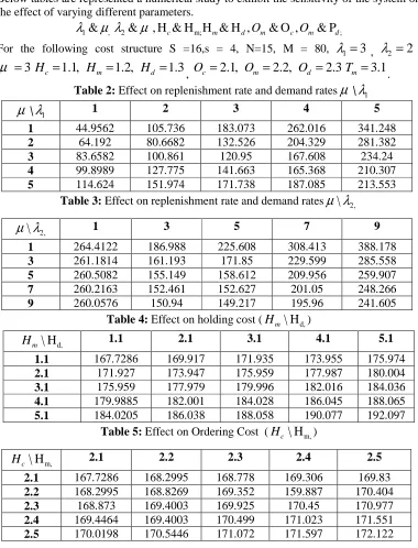
Below tables are represented a numerical study to exhibit the sensitivity of the system on the effect of varying different parameters.
1& , 2& , H & H H & H ,c m; m d Om& O ,c Om& Pd;
λ µ λ
µ
For the following cost structure S =16,s = 4, N=15, M = 80,
λ
1=3,λ
2 =2 ,3
=
µ
Hc =1.1, Hm =1.2, Hd =1.3, Oc=2.1, Om =2.2, Od =2.3Tm =3.1.Table 2: Effect on replenishment rate and demand rates
µ
\λ
1µ
\λ
1 1 2 3 4 51 44.9562 105.736 183.073 262.016 341.248
2 64.192 80.6682 132.526 204.329 281.382
3 83.6582 100.861 120.95 167.608 234.24
4 99.8989 127.775 141.663 165.368 210.307
5 114.624 151.974 171.738 187.085 213.553
Table 3: Effect on replenishment rate and demand rates
µ λ
\ 2,2,
\
µ λ
1 3 5 7 91 264.4122 186.988 225.608 308.413 388.178
3 261.1814 161.193 171.85 229.599 285.558
5 260.5082 155.149 158.612 209.956 259.907
7 260.2163 152.461 152.627 201.05 248.266
9 260.0576 150.94 149.217 195.96 241.605
Table 4: Effect on holding cost (Hm\ Hd,)
d,
\ H
m
H 1.1 2.1 3.1 4.1 5.1
1.1 167.7286 169.917 171.935 173.955 175.974
2.1 171.927 173.947 175.959 177.987 180.004
3.1 175.959 177.979 179.996 182.016 184.036
4.1 179.9885 182.001 184.028 186.045 188.065
5.1 184.0205 186.038 188.058 190.077 192.097
Table 5: Effect on Ordering Cost (Hc \ Hm,)
m,
\ H
c
H 2.1 2.2 2.3 2.4 2.5
2.1 167.7286 168.2995 168.778 169.306 169.83
2.2 168.2995 168.8269 169.352 159.887 170.404
2.3 168.873 169.4003 169.925 170.45 170.977
2.4 169.4464 169.4003 170.499 171.023 171.551 2.5 170.0198 170.5446 171.072 171.597 172.122
Backlogging
165 7. Conclusion
This paper deals with a two echelon Inventory system with two products namely maim and compliment product. The demand at retailer node follows independent Poisson with rate λ1 for main product λ2 for compliment product. If the demand occur for the main
product then it is also the demand for the compliment product. But the compliment product demand do not disturb the main product. The structure of the chain allows vertical movement of goods from to supplier to Retailer. If there is no stock for main product at retailer the demand is backlogged. The model is analyzed within the framework of Markov processes. Joint probability distribution of inventory levels at DC and Retailer for both products are computed in the steady state. Various system performance measures are derived and the long-run expected cost is calculated. By assuming a suitable cost structure on the inventory system, we have presented extensive numerical illustrations to show the effect of change of values on the total expected cost rate. It would be interesting to analyze the problem discussed in this paper by relaxing the assumption of exponentially distributed lead-times to a class of arbitrarily distributed lead-times using techniques from renewal theory and semi-regenerative processes. Once this is done, the general model can be used to generate various special eases.
REFERENCES
1. S.Axsater, Exact and approximate evaluation of batch ordering policies for two level inventory systems, Oper. Res., 41 (1993) 777-785.
2. N.Anbazhagan and G.Arivarignan, Two-commodity continuous review inventory system with coordinated reorder policy, International Journal of Information and Management Sciences, 11(3) (2000) 19 -30.
3. N.Anbazhagan and G.Arivarignan, Analysis of two-commodity Markovian inventory system with lead time, The Korean Journal of Computational and Applied Mathematics, 8(2) (2001) 427- 438.
4. N.Anbazhagan and G.Arivarignan, Two-commodity Markovian inventory system with compliment and retrial demand, British Journal of Mathematics & Computer Science, 3(2) (2013) 115-134.
5. B.M.Beamon, Supply chain design and analysis: models and methods, International Journal of Production Economics, 55(3) (1998) 281-294.
6. E.Cinlar, Introduction to Stochastic Processes, Prentice Hall, Engle-wood Cliffs, NJ, (1975).
7. A.J.Clark and H.Scarf, Optimal policies for a multi- echelon inventory problem, Management Science, 6(4) (1960) 475-490.
8. G.Hadley and T.M.Whitin, Analysis of inventory systems, Prentice-Hall, Englewood Cliff. (1963).
9. F.Harris, Operations and costs, factory management series, A.W.Shah Co., Chicago, 48-52, (1915).
10. S.Kalpakam and G.Arivarigan, A coordinated multicommodity (s, S) inventory system, Mathematical and Computer Modelling, 18 (1993) 69-73.
166
12. A.Krishnamoorthy and T.V.Varghese, A two commodity inventory problem, International Journal of Information and Management Sciences, 5(3) (1994) 55-70.
13. J.Medhi, Stochastic processes, Third edition, New Age International Publishers, New Delhi, (2009).
14. E.Naddor, Inventory System, John Wiley and Sons, New York, (1966).
15. B.D.Sivazlian, Stationary analysis of a multicommodity inventory system with interacting set-up costs, SIAM Journal of Applied Mathematics, 20(2) (1975) 264-278.
16. B.D.Sivazlian and L.E.Stanfel, Analysis of systems in Operations Research, First edition, Prentice Hall, (1974).
17. A.F.Veinott and H.M.Wagner, Computing optimal (s,S) inventory policies, Management Science, 11 (1965) 525-552.
18. A.F.Veinott, The status of mathematical inventory theory, Management Science, 12 (1966) 745-777.
19. V.S.S.Yadavalli, N.Anbazhagan and G.Arivarignan, A two commodity continuous review inventory system with lost sales, Stochastic Analysis and Applications, 22 (2004) 479-497.