DC mod-3.pdf

(1)

Dept. of ISE,CITECH

MODULE 3: TABLE OF CONTENTS

INTRODUCTION

Types of Errors Redundancy

Detection versus Correction Coding

BLOCK CODING

Error Detection

Hamming Distance

Minimum Hamming Distance for Error Detection Linear Block Codes

Minimum Distance for Linear Block Codes Parity-Check Code

CYCLIC CODES

Cyclic Redundancy Check (CRC) Polynomials

Cyclic Code Encoder Using Polynomials Cyclic Code Analysis

Advantages of Cyclic Codes CHECKSUM

Concept of Checksum One's Complement Internet Checksum Algorithm

Other Approaches to the Checksum Fletcher Checksum

Adler Checksum FORWARD ERROR CORRECTION

Using Hamming Distance Using XOR

Chunk Interleaving

Combining Hamming Distance and Interleaving Compounding High- and Low-Resolution Packets DLC SERVICES

Framing

Frame Size

(2)

Flow and Error Control Flow-control

Buffers Error-control

Combination of Flow and Error Control Connectionless and Connection-Oriented

DATA-LINK LAYER PROTOCOLS Simple Protocol

Design FSMs

Stop-and-Wait Protocol Design

FSMs

Sequence and Acknowledgment Numbers Piggybacking

High-level Data Link Control (HDLC)

Configurations and Transfer Modes Framing

Frame Format

Control Fields of HDLC Frames POINT-TO-POINT PROTOCOL (PPP)

Framing

(3)

Chapter 10 Error Detection and Correction

INTRODUCTION Types of Errors

Whenever bits flow from one point to another, they are subject to unpredictable changes because of interference. This interference can change the shape of the signal. In a single-bit error, a 0 is changed to a 1 or a 1 to a 0. In a burst error, multiple bits are changed. For example, a 11100 s burst of impulse noise on a transmission with a data rate of 1200 bps might change all or some of the12 bits of information.

The term single-bit error means that only 1 bit of a given data unit (such as a byte, character, or packet) is changed from 1 to 0 or from 0 to 1. The term burst error means that 2 or more bits in the data unit have changed from 1 to 0 or from 0 to 1.

Redundancy

The central concept in detecting or correcting errors is redundancy. To be able to detect or correct errors, we need to send some extra bits with our data. These redundant bits are added by the sender and removed by the receiver. Their presence allows the receiver to detect or correct corrupted bits.

Detection Versus Correction

The correction of errors is more difficult than the detection. In error detection, we are looking only to see if any error has occurred. The answer is a simple yes or no. We are not even interested in the number of errors. A single-bit error is the same for us as a burst error.

(4)

Forward Error Correction Versus Retransmission

There are two main methods of error correction. Forward error correction is the process in which the receiver tries to guess the message by using redundant bits. This is possible, as we see later, if the number of errors is small. Correction by retransmission is a technique in which the receiver detects the occurrence of an error and asks the sender to resend the message. Resending is repeated until a message arrives that the receiver believes is error-free.

Coding

Redundancy is achieved through various coding schemes. The sender adds redundant bits through a process that creates a relationship between the redundant bits and the actual data bits. The receiver checks the relationships between the two sets of bits to detect or correct the errors. The ratio of redundant bits to the data bits and the robustness of the process are important factors in any coding scheme. Figure 10.3 shows the general idea of coding.

We can divide coding schemes into two broad.

Categories: block coding and convolution coding.

BLOCK CODING

Figure 10.2 shows the role of block coding in error detection. The sender creates code word out of data words by using a generator that applies the rules and procedures of encoding. Each codeword sent to the receiver may change during transmission. If the received codeword is the same as one of the valid code words, the

word is accepted; the corresponding data word is extracted for use. If the received code-word is not valid, it is discarded. However, if the codeword is corrupted during trans-mission but the received word still matches a valid codeword, the error remains undetected.

(5)

and a set of code words, each of size of n. With k bits, we can create a combination of 2k data words; with n bits, we can create a combination of 2n code words. Since n > k, the number of possible code words is larger than the number of possible data words.

The block coding process is one-to-one; the same data word is always encoded as the same codeword. This means that we have 2n - 2k code words that are not used. We call these code words invalid or illegal.

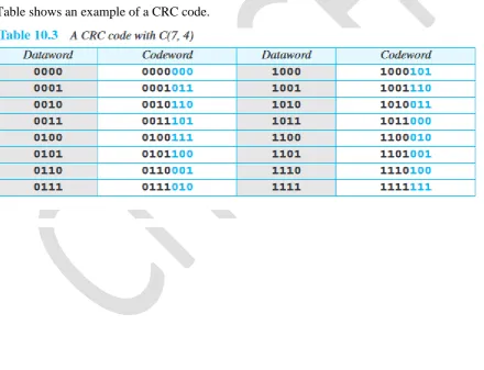
Example

Let us assume that k=2 and n=3. Table 10.1 shows the list of data words and code words. Later, we will see how to derive a codeword from a data word.

Assume the sender encodes the data word 01 as 011 and sends it to the receiver. Consider the following cases:

1. The receiver receives 011. It is a valid codeword. The receiver extracts the dataword 01 from it.

2. The codeword is corrupted during transmission, and 111 is received (the leftmost bit is corrupted). This is not a valid codeword and is discarded.

3. The codeword is corrupted during transmission, and 000 is received (the right two bits are corrupted). This is a valid codeword. The receiver incorrectly extracts the data word 00. Two corrupted bits have made the error undetectable.

Hamming Distance

One of the central concepts in coding for error control is the idea of the Hamming distance. The Hamming distance between two words (of the same size) is the number of differences between the corresponding bits. We show the Hamming distance between two words x and y as d(x, y). The Hamming distance can easily be found if we apply the XOR operation on the two words and count the number of Is in the result. Note that the Hamming distance is a value greater than zero.

Minimum Hamming Distance

Although the concept of the Hamming distance is the central point in dealing with error detection and correction codes, the measurement that is used for designing a code is the minimum Hamming distance. In a set of words, the minimum Hamming distance is the smallest Hamming distance between all possible pairs. We use dmin to define the minimum Hamming distance in a coding scheme. To find this value, we find the Hamming distances between all words and select the smallest one.

(6)

for dmin- For example, we can call our first coding scheme C(3, 2) with dmin =2 and our second coding scheme C(5, 2) with dmin ::= 3.

Hamming Distance and Error

Before we explore the criteria for error detection or correction, let us discuss the relationship between the Hamming distance and errors occurring during transmission. When a codeword is corrupted during transmission, the Hamming distance between the sent and received code words is the number of bits affected by the error. In other words, the Hamming distance between the received codeword and the sent codeword is the number of bits that are corrupted during transmission. For example, if the codeword 00000 is sent and 01101 is received, 3 bits are in error and the Hamming distance between the two is d(OOOOO, 01101) =3.

Minimum Distance for Error Detection

Now let us find the minimum Hamming distance in a code if we want to be able to detect up to s errors. If s errors occur during transmission, the Hamming distance between the sent codeword and received codeword is s. If our code is to detect up to s errors, the minimum distance between the valid codes must be s + 1, so that the received codeword does not match a valid codeword. In other words, if the minimum distance between all valid codewords is s + 1, the received codeword cannot be erroneously mistaken for another codeword. The distances are not enough (s + 1) for the receiver to accept it as valid. The error will be detected. We need to clarify a point here: Although a code with dmin =s + 1

Minimum Distance for Error Correction

Error correction is more complex than error detection; a decision is involved. When a received codeword is not a valid codeword, the receiver needs to decide which valid codeword was actually sent. The decision is based on the concept of territory, an exclusive area surrounding the codeword. Each valid codeword has its own territory. We use a geometric approach to define each territory. We assume that each valid codeword has a circular territory with a radius of t and that the valid codeword is at the center. For example, suppose a codeword x is corrupted by t bits or less. Then this corrupted codeword is located either inside or on the perimeter of this circle. If the receiver receives a codeword that belongs to this territory, it decides that the original codeword is the one at the center. Note that we assume that only up to t errors have occurred; otherwise, the decision is wrong. Figure 10.9 shows this geometric interpretation. Some texts use a sphere to show the distance between all valid block codes.

LINEAR BLOCK CODES

Almost all block codes used today belong to a subset called linear block codes. The use of nonlinear block codes for error detection and correction is not as widespread because their

(7)

Minimum Distance for Linear Block Codes

It is simple to find the minimum Hamming distance for a linear block code. The minimum Hamming distance is the number of Is in the nonzero valid codeword with the smallest number of 1s.

Some Linear Block Codes

Let us now show some linear block codes. These codes are trivial because we can easily find the encoding and decoding algorithms and check their performances.

Simple Parity-Check Code

(8)

This is normally done by adding the 4 bits of the dataword (modulo-2); the result is the parity bit. In other words,

If the number of 1s is even, the result is 0; if the number of 1s is odd, the result is 1. In both cases, the total number of 1s in the codeword is even. The sender sends the codeword which may be corrupted during transmission. The receiver receives a 5-bit word. The checker at the receiver does the same thing as the generator in the sender with one exception: The addition is done over all 5 bits. The result, which is called the syndrome, is just 1 bit. The syndrome is 0 when the number of 1s in the received codeword is even; otherwise, it is 1.

The syndrome is passed to the decision logic analyzer. If the syndrome is 0, there is no error in the received codeword; the data portion of the received codeword is accepted as the data word; if the syndrome is 1, the data portion of the received codeword is discarded. The data word is not created.

Example

Let us look at some transmission scenarios. Assume the sender sends the data word 1011. The codeword created from this dataword is 10111, which is sent to the receiver. We examine five cases:

1. No error occurs; the received codeword is 10111. The syndrome is 0. The data word 1011 is created.

2. One single-bit error changes a1, the received codeword is 10011. The syndrome is 1. No data word is created.

3. One single-bit error changes r0, the received codeword is 10110. The syndrome is 1. No data word is created. Note that although none of the data word bits are corrupted, no data word is created because the code is not sophisticated enough to show the position of the corrupted bit.

4. An error changes ro and a second error changes a3,the received codeword is 00110. The syndrome is 0. The data word 0011 is created at the receiver. Note that here the data word is wrongly created due to the syndrome value. The simple parity-check decoder cannot detect an even number of errors. The errors cancel each other out and give the syndrome a value of 0.

5. Three bits-a3, a2, and a1- are changed by errors. The received codeword is 01011. The syndrome is 1. The data word is not created. This shows that the simple parity check, guaranteed to detect one single error, can also find any odd number of errors.

(9)

CYCLIC CODES

Cyclic codes are special linear block codes with one extra property. In a cyclic code, if a codeword is cyclically shifted (rotated), the result is another codeword. For example, if 1011000 is a codeword and we cyclically left-shift, then 0110001 is also a codeword.

In this case, if we call the bits in the first word ao to a6' and the bits in the second word B0 to b6, we can shift the bits by using the following:

In the rightmost equation, the last bit of the first word is wrapped around and becomes the first bit of the second word.

Cyclic Redundancy Check

We can create cyclic codes to correct errors. However, the theoretical background required is beyond the scope of this book. In this section, we simply discuss a category of cyclic codes called the cyclic redundancy check (CRC) that is used in networks such as LANs and WANs.

(10)

(11)

Dept. of ISE,CITECH Encoder

Let us take a closer look at the encoder. The encoder takes the data word and augments it with n - k number of as. It then divides the augmented data word by the divisor, as shown in Figure.

The process of modulo-2 binary division is the same as the familiar division process we use for decimal numbers. However, as mentioned at the beginning of the chapter, in this case addition and subtraction are the same. We use the XOR operation to do both. As in decimal division, the process is done step by step. In each step, a copy of the divisor is XORed with the 4 bits of the dividend. The result of the XOR operation (remainder) is 3 bits (in this case), which is used for the next step after 1 extra bit is pulled down to make it 4 bits long. There is one important point we need to remember in this type of division. If the leftmost bit of the dividend (or the part used in each step) is 0, the step cannot use the regular divisor; we need to use an all-0s divisor. When there are no bits left to pull down, we have a result. The 3-bit remainder forms the check bits (r2 r1 and r0). They are appended to the data word to create the codeword.

Decoder

(12)

of syndrome when no error has occurred; the syndrome is 000. The right-hand part of the figure shows the case in which there is one single error. The syndrome is not all 0s (it is 01l).

Polynomials

(13)

Figure shows one immediate benefit; a 7-bit pattern can be replaced by three terms. The benefit is even more conspicuous when we have a polynomial such as x23 + X3 + 1. Here the bit pattern is 24 bits in length (three Is and twenty-one Os) while the polynomial is just three terms.

Degree of a Polynomial

The degree of a polynomial is the highest power in the polynomial. For example, the degree of the polynomial x6 + x + 1 is 6. Note that the degree of a polynomial is 1 less that the number of bits in the pattern. The bit pattern in this case has 7 bits.

Adding and Subtracting Polynomials

Adding and subtracting polynomials in mathematics are done by adding or subtracting the coefficients of terms with the same power. In our case, the coefficients are only 0 and 1, and adding is in modulo-2. This has two consequences. First, addition and subtraction are the same. Second, adding or subtracting is done by combining terms and deleting pairs of identical terms. For example, adding x5 + x4_{+ x}2_{and x}6_{+ x}4_{+ x}2_{gives just x}6_{+ x}5_{. The terms}

x4 and x2 are deleted. However, note that if we add, for example, three polynomials and we get x2 three times, we delete a pair of them and keep the third.

Multiplying or Dividing Terms

In this arithmetic, multiplying a term by another term is very simple; we just add the powers. For example, x3_*_x4_{is x}7_{, For dividing, we just subtract the power of the second term from}

the power of the first. For example, x5 / x2_{is x}3_.

Multiplying Two Polynomials

Multiplying a polynomial by another is done term by term. Each term of the first polynomial must be multiplied by all terms of the second. The result, of course, is then simplified, and pairs of equal terms are deleted. The following is an example:

Dividing One Polynomial by Another

Division of polynomials is conceptually the same as the binary division we discussed for an encoder. We divide the first term of the dividend by the first term of the divisor to get the first term of the quotient. We multiply the term in the quotient by the divisor and subtract the result from the dividend. We repeat the process until the dividend degree is less than the divisor degree. We will show an example of division later in this chapter.

Cyclic Code Encoder Using Polynomials

Now that we have discussed operations on polynomials, we show the creation of a codeword from a data word. Figure 10.22 is the polynomial version of Figure 10.15. We can see that the process is shorter. The data word 1001 is represented as x3 + 1. The divisor 1011 is represented as x3 + x + 1. To find the augmented data word, we have left-shifted the data word 3 bits (multiplying by x\ The result is x6+ x3_{. Division is straightforward. We divide the}

(14)

is then x6/x3, or x3. Then we multiply x3 by the divisor and subtract (according to our previous definition of subtraction) the result from the dividend. The result is x4_,_{with a degree greater}

than the divisor's degree; we continue to divide until the degree of the remainder is less than the degree of the divisor.

It can be seen that the polynomial representation can easily simplify the operation of division in this case, because the two steps involving all-Os divisors are not needed here. (Of course, one could argue that the all-Os divisor step can also be eliminated in binary division.) In a polynomial representation, the divisor is normally referred to as the generator polynomial t(x).

Cyclic Code Analysis

We can analyze a cyclic code to find its capabilities by using polynomials. We define the following, where f(x) is a polynomial with binary coefficients.

Dataword: d(x)

Syndrome: s(x)

Codeword: c(x)

Error: e(x)

Generator: g(x)

(15)

In our analysis we want to find the criteria that must be imposed on the generator, g(x) to detect the type of error we especially want to be detected. Let us first find the relationship among the sent codeword, error, received codeword, and the generator. We can say

Received codeword =c(x) +e(x)

In other words, the received codeword is the sum of the sent codeword and the error. The receiver divides the received codeword by g(x) to get the syndrome. We can write this as

The first term at the right-hand side of the equality does not have a remainder (according to the definition of codeword). So the syndrome is actually the remainder of the second term on the right-hand side. If this term does not have a remainder (syndrome =0), either e(x) is 0 or e(x) is divisible by g(x). We do not have to worry about the first case (there is no error); the second case is very important. Those errors that are divisible by g(x) are not caught. Let us show some specific errors and see how they can be caught by a well designed g(x).

Single-Bit Error

What should be the structure of g(x) to guarantee the detection of a bit error? A single-bit error is e(x) =xi, where i is the position of the bit. If a single-bit error is caught, then xi is not divisible by g(x). (Note that when we say not divisible, we mean that there is a

remainder.) If g(x) ha~at least two terms (which is normally the case) and the coefficient of x0 is not zero(the rightmost bit is 1), then e(x) cannot be divided by g(x).

Two Isolated Single-Bit Errors

(16)

Dept. of ISE,CITECH Odd Numbers of Errors

A generator with a factor of x + 1 can catch all odd numbers of errors. This means that we need to make x + 1 a factor of any generator. Note that we are not saying that the generator itself should be x + 1; we are saying that it should have a factor of x + 1. If it is only x + 1, it cannot catch the two adjacent isolated errors (see the previous section). For example, x4 + x2 + X + 1 can catch all odd-numbered errors since it can be written as a product of the two polynomials x + 1 and x3 + x2 + 1.

Burst Errors

Now let us extend our analysis to the burst error, which is the most important of all. A burst error is of the form e(x) =eJ + ... + xi). Note the difference between a burst error and two isolated single-bit errors. The first can have two terms or more; the second can only have two terms. We can factor out xi and write the error as xi(xJ-i + ... + 1). If our generator can detect a single error (minimum condition for a generator), then it cannot divide xi. What we should worry about are those generators that divide xJ-i + ... + 1. In other words, the remainder of (xJ-i + ... + 1)/(xr +... + 1) must not be zero. Note that the denominator is the generator polynomial.

We can have three cases:

1. If j - i < r, the remainder can never be zero. We can write j - i =L - 1, where L is the length of the error. So L - 1 < r or L < r + 1 or L :::;: r. This means all burst errors with length smaller than or equal to the number of check bits r will be detected.

2. In some rare cases, if j - i = r, or L = r + 1, the syndrome is 0 and the error is undetected. It can be proved that in these cases, the probability of undetected burst error of length r + 1 is

(ll2r-l. For example, if our generator is x l4 + ~ + 1, in which r =14, aburst error of length L

=15 can slip by undetected with the probability of (1/2)14-1 or almost 1 in 10,000.

(17)

Dept. of ISE,CITECH Standard Polynomials

(18)

Advantages of Cyclic Codes

(19)

Other Cyclic Codes

The cyclic codes we have discussed in this section are very simple. The check bits and syndromes can be calculated by simple algebra. There are, however, more powerful polynomials that are based on abstract algebra involving Galois fields. These are beyond the scope of this book. One of the most interesting of these codes is the Reed-Solomon code used today for both detection and correction.

CHECKSUM

The last error detection method we discuss here is called the checksum. The checksum is used in the Internet by several protocols although not at the data link layer. However,we briefly discuss it here to complete our discussion on error checking. Like linear and cyclic codes, the checksum is based on the concept of redundancy. Several protocols still use the checksum for error detection although the tendency is to replace it with a CRC. This means that the CRC is also used in layers other than the data link layer.

Idea

The concept of the checksum is not difficult. Let us illustrate it with a few examples. One's Complement The previous example has one major drawback. All of our data can be written as a 4-bit word (they are less than 15) except for the checksum. One solution is to use one's complement arithmetic. In this arithmetic, we can represent unsigned numbers between 0 and 2n - 1 using only n bits. t If the number has more than n bits, the extra leftmost bits need to be added to the n rightmost bits (wrapping). In one's complement arithmetic, a negative number can be represented by inverting all bits (changing a 0 to a 1 and a 1 to a 0). This is the same as subtracting the number from 2n - 1.

Internet Checksum

Traditionally, the Internet has been using a 16-bit checksum. The sender calculates the checksum by following these steps.

Sender site:

1. The message is divided into 16-bit words. 2. The value of the checksum word is set to O.

3. All words including the checksum are added ushtg one's complement addition. 4. The sum is complemented and becomes the checksum.

5. The checksum is sent with the data.

Receiver site:

1. The message (including checksum) is divided into 16-bit words.

2. All words are added using one's complement addition. 3. The sum is complemented and becomes the new checksum.

(20)

At the source, the message is first divided into m-bit units. The generator then creates an extra m-bit unit called the checksum, which is sent with the message. At the destination, the checker creates a new checksum from the combination of the message and sent checksum. If the new checksum is all 0s, the message is accepted; otherwise, the message is discarded (Figure 10.15). Note that in the real implementation, the checksum unit is not necessarily added at the end of the message; it can be inserted in

the middle of the message.

Concept

The idea of the traditional checksum is simple. We show this using a simple example. Example 10.11 Suppose the message is a list of five 4-bit numbers that we want to send to a destination. In addition to sending these numbers , we send the sum of the numbers. For example, if the set of numbers is (7, 11, 12, 0, 6), we send (7, 11, 12, 0, 6, 36), where 36 is the sum of the original numbers. The receiver adds the five numbers and compares the result with the sum. If the two are the same, the receiver assumes no error, accepts the five numbers, and discards the sum. Otherwise, there is an error somewhere and the message is not accepted. One’s Complement Addition The previous example has one major drawback. Each number can be written as a 4-bit word (each is less than 15) except for the sum. One solution is to use one’s complement arithmetic. In this arithmetic, we

can represent unsigned numbers between 0 and 2m−1 using only m bits. If the number

has more than m bits, the extra leftmost bits need to be added to the m rightmost bits (wrapping).

(21)

Checksum

We can make the job of the receiver easier if we send the complement of the sum, the checksum. In one’s complement arithmetic, the complement of a number is found by completing all bits (changing all 1s to 0s and all 0s to 1s). This is the same as subtracting the number from 2m−1. In one’s complement arithmetic, we have two 0s: one positive and one negative, which are complements of each other. The positive zero has all m bits set to 0; the negative zero has all bits set to 1 (it is 2m− 1). If we add a number with its complement, we get a negative zero (a number with all bits set to 1). When the receiver adds all five numbers (including the checksum), it gets a negative zero. The receiver can complement the result again to get a positive zero.

Example

Let us use the idea of the checksum in Example. The sender adds all five numbers in one’s complement to get the sum = 6. The sender then complements the result to get the checksum =9, which is 15 −6. Note that 6 =(0110)2 and 9 =(1001)2; they are complements of each other. The sender sends the five data numbers and the checksum (7, 11, 12, 0, 6, 9). If there is no corruption in transmission, the receiver receives (7, 11, 12, 0, 6, 9) and adds them in one’s complement to get 15.The sender complements 15 to get 0. This shows that data have not been corrupted. Figure shows the process.

Internet Checksum

(22)

Algorithm

(23)

Other Approaches to the Checksum

As mentioned before, there is one major problem with the traditional checksum calculation. If two 16-bit items are transposed in transmission, the checksum cannot catch this error. The reason is that the traditional checksum is not weighted: it treats each data item equally. In other words, the order of data items is immaterial to the calculation. Several approaches have been used to prevent this problem. We mention two of them here: Fletcher and Adler.

Fletcher Checksum

The Fletcher checksum was devised to weight each data item according to its position. Fletcher has proposed two algorithms: 8-bit and 16-bit. The first, 8-bit Fletcher, calculates on 8-bit data items and creates a bit checksum. The second, bit Fletcher, calculates on 16-bit data items and creates a 32-16-bit checksum. The 8-16-bit Fletcher is calculated over data octets (bytes) and creates a 16-bit check-sum. The calculation is done modulo 256 (28), which means the intermediate results are divided by 256 and the remainder is kept. The algorithm uses two accumulators, L and R. The first simply adds data items together; the second adds a weight to the calculation. There are many variations of the 8-bit Fletcher algorithm; we show a simple one in Figure 10.18. The 16-bit Fletcher checksum is similar to the 8-bit Fletcher checksum, but it is calculated over 16-bit data items and creates a 32-bit checksum. The calculation is done modulo 65,536.

Adler Checksum

(24)

FORWARD ERROR CORRECTION

We discussed error detection and retransmission in the previous sections. However, retransmission of corrupted and lost packets is not useful for real-time multimedia transmission because it creates an unacceptable delay in reproducing: we need to wait until the lost or corrupted packet is resent. We need to correct the error or reproduce the packet immediately. Several schemes have been designed and used in this case that are collectively referred to as forward error correction (FEC) techniques. We briefly discuss some of the common techniques here.

Using Hamming Distance

We earlier discussed the Hamming distance for error detection. We said that to detect

s errors, the minimum Hamming distance should be dmin=s+1. For error detection, we

definitely need more distance. It can be shown that to detect t errors, we need to have

dmin=2t+1. In other words, if we want to correct 10 bits in a packet, we need to make

(25)

Using XOR

Another recommendation is to use the property of the exclusive OR operation as shown below.

R=P1⊕P2⊕... ⊕ Pi ⊕...⊕PN → Pi=P1⊕P2⊕...⊕R ⊕ ...⊕PN

In other words, if we apply the exclusive OR operation on N data items (P1to PN), we can recreate any of the data items by exclusive-ORing all of the items, replacing the one to be created by the result of the previous operation (R). This means that we can divide a packet into N chunks, create the exclusive OR of all the chunks and send N+1 chunks. If any chunk is lost or corrupted, it can be created at the receiver site. Now the question is what should the value of N be. If N= 4, it means that we need to send 25 percent extra data and be able to correct the data if only one out of four chunks is lost.

Chunk Interleaving

(26)

Compounding High- and Low-Resolution Packets

(27)

CHAPTER 11 DATA LINK CONTROL

DLC Services

 DLC deals with procedures for communication between two adjacent nodes.(dedicated or broadcast).

 DLC functions include framing and flow and error control.

Frames

 The data-link layer needs to pack bits into frames, so that each frame is

distinguishable from another.

 Framing in the data-link layer separates a message from one source to a

destination by adding a sender address and a destination address. The destination address defines where the packet is to go; the sender address helps the recipient acknowledge the receipt.

Frame Size

 Frames can be of fixed or variable size.

 In fixed-size framing, there is no need for defining the boundaries of the

frames; the size itself can be used as a delimiter.

 An example of this type of framing is the ATM WAN, which uses frames of

fixed size called cells. .

 Variable size framing, prevalent in local-area networks. In variable-size

framing, we need a way to define the end of one frame and the beginning of the next.

 Historically, two approaches were used for this purpose: a character-oriented

approach and a bit oriented approach.

Character-Oriented Framing

 In character-oriented (or byte-oriented) framing, data to be carried are 8-bit

characters from a coding system such as ASCII.

 The header, which normally carries the source and destination addresses and

other control information, and the trailer, which carries error detection redundant bits, are also multiples of 8 bits.

 To separate one frame from the next, an 8-bit (1-byte) flag is added at the

(28)

 Any character used for the flag could also be part of the information.

 If this happens, the receiver, when it encounters this pattern in the middle of the data, thinks it has reached the end of the frame.

 To fix this problem, a byte-stuffing strategy was added to character oriented framing.

 In byte stuffing (or character stuffing), a special byte is added to the data section of the frame when there is a character with the same pattern as the flag.

 The data section is stuffed with an extra byte. This byte is usually called the escape character (ESC) and has a predefined bit pattern.

 Whenever the receiver encounters the ESC character, it removes it from the data section and treats the next character as data, not as a delimiting flag.

Bit-Oriented Framing

 In bit-oriented framing, the data section of a frame is a sequence of bits to be

interpreted by the upper layer as text, graphic, audio, video, and so on.

 In addition to headers (and possible trailers), we still need a delimiter to

separate one frame from the other.

 Most protocols use a special 8-bit pattern flag, 01111110, as the delimiter to

(29)

 If the flag pattern appears in the data, we need to somehow inform the receiver

that this is not the end of the frame.

 We do this by stuffing 1 single bit (instead of 1 byte) to prevent the pattern

from looking like a flag.

 The strategy is called bit stuffing.

 In bit stuffing, if a 0 and five consecutive 1 bits are encountered, an extra 0 is

added.

 This extra stuffed bit is eventually removed from the data by the receiver.

 Note that the extra bit is added after one 0 followed by five 1s regardless of the

value of the next bit.

 This guarantees that the flag field sequence does not inadvertently appear in the

frame.

(30)

Flow and Error Control

Flow Control

 Whenever an entity produces items and another entity consumes them, there

should be a balance between production and consumption rates.

 If the items are produced faster than they can be consumed, the consumer can

be overwhelmed and may need to discard some items.

 If the items are produced more slowly than they can be consumed, the

consumer must wait, and the system becomes less efficient.

 Flow control is related to the first issue.

 We need to prevent losing the data items at the consumer site.

The figure shows that the data-link layer at the sending node tries to push frames toward the data-link layer at the receiving node. If the receiving node cannot process and deliver the packet to its network at the same rate that the frames arrive, it becomes overwhelmed with frames. Flow control in this case can be feedback from the receiving node to the sending node to stop or slow down pushing frames.

Buffers

Although flow control can be implemented in several ways, one of the solutions is normally to use two buffers; one at the sending data-link layer and the other at the receiving data-link layer. A buffer is a set of memory locations that can hold packets at the sender and receiver. The flow control communication can occur by sending signals from the consumer to the producer. When the buffer of the receiving data-link layer is full, it informs the sending data-link layer to stop pushing frames.

Connectionless and Connection-Oriented

Connectionless Protocol

 In a connectionless protocol, frames are sent from one node to the next without any relationship between the frames; each frame is independent.

 Connectionless means that there is no connection between frames.

 The frames are not numbered and there is no sense of ordering.

(31)

Connection oriented Protocol

 In a connection-oriented protocol, a logical connection should first be established between the two nodes (setup phase).

 After all frames that are somehow related to each other are transmitted (transfer phase)

 The logical connection is terminated (teardown phase).

 Connection-oriented protocols are rare in wired LANs, but we can see them in some point-to-point protocols, some wireless LANs, and some WANs.

Data Link Layer Protocols

Simple Protocol

 First protocol is a simple protocol with neither flow nor error control.

 The data-link layer at the sender gets a packet from its network layer, makes a frame out of it, and sends the frame.

 The data-link layer at the receiver receives a frame from the link, extracts the packet from the frame, and delivers the packet to its network layer.

 The data-link layers of the sender and receiver provide transmission services for their network layers.

(32)

 The sender site should not send a frame until its network layer has a message to send. The receiver site cannot deliver a message to its network layer until a frame arrives. We can show these requirements using two FSMs.

 Each FSM has only one state, the ready state.

 The sending machine remains in the ready state until a request comes from the process in the network layer.

 When this event occurs, the sending machine encapsulates the message in a frame and sends it to the receiving machine.

 The receiving machine remains in the ready state until a frame arrives from the sending machine.

 When this event occurs, the receiving machine decapsulates the message out of the frame and delivers it to the process at the network layer.

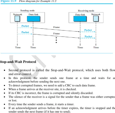
Figure shows an example of communication using this protocol. It is very simple. The sender sends frames one after another without even thinking about the receiver.

Stop-and-Wait Protocol

 Second protocol is called the Stop-and-Wait protocol, which uses both flow

and error control.

 In this protocol, the sender sends one frame at a time and waits for an acknowledgment before sending the next one.

 To detect corrupted frames, we need to add a CRC to each data frame.

 When a frame arrives at the receiver site, it is checked.

 If its CRC is incorrect, the frame is corrupted and silently discarded.

 The silence of the receiver is a signal for the sender that a frame was either corrupted or lost.

 Every time the sender sends a frame, it starts a timer.

 If an acknowledgment arrives before the timer expires, the timer is stopped and the sender sends the next frame (if it has one to send).

(33)

 This means that the sender needs to keep a copy of the frame until its acknowledgment arrives.

 When the corresponding acknowledgment arrives, the sender discards the copy and sends the next frame if it is ready.

 Figure shows the outline for the Stop-and-Wait protocol.

 Note that only one frame and one acknowledgment can be in the channels at any time.

(34)

We describe the sender and receiver states below.

Sender States

The sender is initially in the ready state, but it can move between the ready and blocking state.

Ready State

 When the sender is in this state, it is only waiting for a packet from the network layer.

 If a packet comes from the network layer, the sender creates a frame, saves a copy of the frame, starts the only timer and sends the frame.

 The sender then moves to the blocking state.

Blocking State: When the sender is in this state, three events can occur

 If a time-out occurs, the sender resends the saved copy of the frame and restarts the timer.

 If a corrupted ACK arrives, it is discarded.

 If an error-free ACK arrives, the sender stops the timer and discards the saved copy of the frame. It then moves to the ready state.

Receiver

The receiver is always in the ready state. Two events may occur:

a. If an error-free frame arrives, the message in the frame is delivered to the network layer and an ACK is sent.

b. If a corrupted frame arrives, the frame is discarded.

(35)

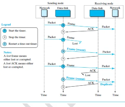
Sequence and Acknowledgment Numbers

 We need to add sequence numbers to the data frames and acknowledgment numbers to the ACK frames.

 Sequence numbers are 0, 1, 0, 1, 0, 1, . . . ; the acknowledgment numbers can also be 1, 0, 1, 0, 1, 0, ...

 In other words, the sequence numbers start with 0, the acknowledgment numbers start with 1. An acknowledgment number always defines the sequence number of the next frame to receive.

Figure shows how adding sequence numbers and acknowledgment numbers can prevent duplicates. The first frame is sent and acknowledged. The second frame is sent, but lost. After time-out, it is resent. The third frame is sent and acknowledged, but the acknowledgment is lost. The frame is resent.

(36)

HDLC

High-level Data Link Control (HDLC) is a bit-oriented protocol for communication over point-to-point and multipoint links.

Configurations and Transfer Modes

(37)

Framing

 To provide the flexibility necessary to support all the options possible in the

modes and configurations just described, HDLC defines three types of frames:

 Information frames (I-frames) , supervisory frames (S-frames), and

unnumbered frames (U frames).

 Each type of frame serves as an envelope for the transmission of a different

type of message.

 I-frames are used to data-link user data and control information relating to user

data (piggy-backing).

 S-frames are used only to transport control information.

 U frames are reserved for system management.

 Information carried by U-frames is intended for managing the link itself.

 Each frame in HDLC may contain up to six fields, as shown in Figure a beginning flag field, an address field, a control field, an information field, a frame check sequence (FCS) field, and an ending flag field.

(38)

Flag field

This field contains synchronization pattern 01111110, which identifies both the beginning and the end of a frame.

Address field

This field contains the address of the secondary station. If a primary station created the frame, it contains a to address. If a secondary station creates the frame, it contains a from address. The address field can be one byte or several bytes long, depending on the needs of the network.

Control field

The control field is one or two bytes used for flow and error control.

Information field

The information field contains the user’s data from the network layer or management information. Its length can vary from one network to another.

FCS field

The frame check sequence (FCS) is the HDLC error detection field. It can contain either a 2- or 4-byte CRC.

The control field determines the type of frame and defines its functionality

Control Field for I-Frames

 I-frames are designed to carry user data from the network layer.

 In addition, they can include flow- and error-control information (piggybacking).

 The subfields in the control field are used to define these functions.

 The first bit defines the type.

 If the first bit of the control field is 0, this means the frame is an I-frame.

 The next 3 bits, called N(S), define the sequence number of the frame.

(39)

 The last 3 bits, called N(R), correspond to the acknowledgment number when piggybacking is used.

 The single bit between N(S) and N(R) is called the P/F bit.

 The P/F field is a single bit with a dual purpose.

 It has meaning only when it is set (bit =1) and can mean poll or final.

 It means poll when the frame is sent by a primary station to a secondary (when the address field contains the address of the receiver).

 It means final when the frame is sent by a secondary to a primary (when the address field contains the address of the sender).

Control Field for S-Frames

 Supervisory frames are used for flow and error control whenever piggybacking

is either impossible or inappropriate.

 S-frames do not have information fields.

 If the first 2 bits of the control field are 10, this means the frame is an S-frame.

 The last 3 bits, called N(R), correspond to the acknowledgment number (ACK)

or negative acknowledgment number (NAK), depending on the type of S-frame.

 The 2 bits called code are used to define the type of S-frame itself.

 With 2 bits, we can have four types of S-frames, as described below:

Receive ready (RR)

 If the value of the code subfield is 00, it is an RR S-frame.

 This kind of frame acknowledges the receipt of a safe and sound frame or group of frames.

 In this case, the value of the N(R) field defines the acknowledgment number.

Receive not ready (RNR)

 If the value of the code subfield is 10, it is an RNR S-frame.

 This kind of frame is an RR frame with additional functions.

 It acknowledges the receipt of a frame or group of frames, and it announces that the receiver is busy and cannot receive more frames. It acts as a kind of congestion control mechanism by asking the sender to slow down. The value of N(R) is the acknowledgment number.

Reject (REJ)

 If the value of the code subfield is 01, it is an REJ S-frame.

 This is a NAK frame, but not like the one used for Selective Repeat ARQ.

 It is a NAK that can be used in Go-Back-N ARQ to improve the efficiency of the process by informing the sender, before the sender timer expires, that the last frame is lost or damaged.

(40)

Selective reject (SREJ)

 If the value of the code subfield is 11, it is an SREJ S-frame.

 This is a NAK frame used in Selective Repeat ARQ.

 Note that the HDLC Protocol uses the term selective reject instead of selective repeat.

 The value of N(R) is the negative acknowledgment number.

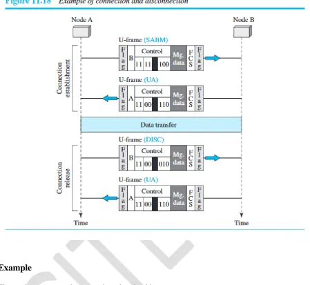
Control Field for U-Frames

 Unnumbered frames are used to exchange session management and control information between connected devices.

 U-frames contain an information field, but one used for system management information, not user data.

(41)

Example

Figure shows two exchanges using piggybacking.

(42)

POINT-TO-POINT PROTOCOL (PPP)

One of the most common protocols for point-to-point access is the Point-to-Point Protocol (PPP).

Services

Services Provided by PPP

 PPP does not provide flow control.

 A sender can send several frames one after another with no concern about overwhelming the receiver.

 PPP has a very simple mechanism for error control.

 A CRC field is used to detect errors. If the frame is corrupted, it is silently discarded; the upper-layer protocol needs to take care of the problem.

(43)

 PPP does not provide a sophisticated addressing mechanism to handle frames in a multipoint configuration.

Framing

PPP uses a character-oriented (or byte-oriented) frame. Figure shows the format of a PPP frame. The description of each field follows:

Address

The address field in this protocol is a constant value and set to 11111111 (broadcast address).

Control

This field is set to the constant value 00000011 (imitating unnumbered frames in HDLC). As we will discuss later, PPP does not provide any flow control. Error control is also limited to error detection.

Protocol

The protocol field defines what is being carried in the data field: either user data or other information. This field is by default 2 bytes long, but the two parties can agree to use only 1 byte.

Payload field

This field carries either the user data or other information that we will discuss shortly. The data field is a sequence of bytes with the default of a maximum of 1500 bytes; but this can be changed during negotiation. The data field is byte-stuffed if the flag byte pattern appears in this field. Because there is no field defining the size of the data field, padding is needed if the size is less than the maximum default value or the maximum negotiated value.

FCS

(44)

Transition Phases

 A PPP connection goes through phases which can be shown in a transition

phase diagram.

 The transition diagram, which is an FSM, starts with the dead state.

 In dead state, there is no active carrier (at the physical layer) and the line is quiet. When one of the two nodes starts the communication, the connection

goes into the establish state.

 In establish state, options are negotiated between the two parties.

 If the two parties agree that they need authentication (for example, if they do

not know each other), then the system needs to do authentication (an extra step); otherwise, the parties can simply start communication.

 Data transfer takes place in the open state.

 When a connection reaches open state, the exchange of data packets can be

started.

 The connection remains in open state until one of the end points wants to

terminate the connection.

 In this case, the system goes to the terminate state. The system remains in this

state until the carrier (physical-layer signal) is dropped, which moves the

(45)

MODULE 3: ERROR-DETECTION AND CORRECTION

1.Explain two types of errors (4*)

2.Compare error detection vs. error correction (2)

3.Explain error detection using block coding technique. (10*) 4.Explain hamming distance for error detection (6*)

5.Explain parity-check code with block diagram. (6*) 6.Explain CRC with block diagram & an example. (10*) 7.Write short notes on polynomial codes. (5*)

8.Explain internet checksum algorithm along with an example. (6*) 9.Explain the following:

Fletcher checksum and ii) Adler checksum (8) 10.Explain various FEC techniques. (6)

MODULE 3: DATA LINK CONTROL

1.Explain two types of frames. (2)

2.Explain character oriented protocol. (6*)

3.Explain the concept of byte stuffing and unstuffing with example. (6*)

4.Explain bit oriented protocol. (6*)

5.Differentiate between character oriented and bit oriented format for Framing. (6*)

6.Compare flow control and error control. (4)

7.With a neat diagram, explain the design of the simplest protocol with no flow control. (6)

8.Write algorithm for sender site and receiver site for the simplest protocol. (6)

9.Explain Stop-and-Wait protocol (8*)

10.Explain the concept of Piggybacking (2*) 11.Explain in detail HDLC frame format. (8*) 12.Explain 3 type of frame used in HDLC (8*)