Application example Given a graph representation and a vertex sin the graph Find all paths from sto other vertices

DATA STRUCTURES

AND ALGORITHMS

◻

Graph Traversal

Graph Traversal

◻

Application example

Given a graph representation and a vertex

s

in the graph

Find all paths from

s

to other vertices

◻

Two common graph traversal algorithms

■

Breadth-First Search (BFS)

■

Find the shortest paths in an unweight graph

■

Depth-First Search (DFS)

■

Topological sort

■

Find strongly connected components

BFS and Shortest Path Problem

◻

Given any source vertex s, BFS visits the other vertices at

increasing distances away from s. In doing so, BFS discovers

paths from s to other vertices

◻

What do we mean by “distance”? The number of edges on a

path from s.

2

4

3

5 1

7

6 9

8 0

Consider s=vertex 1

Nodes at distance 1? 2, 3, 7, 9

1

1 1

1 2

2 2

2

s

Example

Nodes at distance 2? 8, 6, 5, 4

BSF algorithm

Example

2

4

3

5 1

7

6 9

8 0

Adjacency List

source

0 1 2 3 4 5 6 7 8 9

Visited Table (T/F)

F

F

F

F

F

F

F

F

F

F

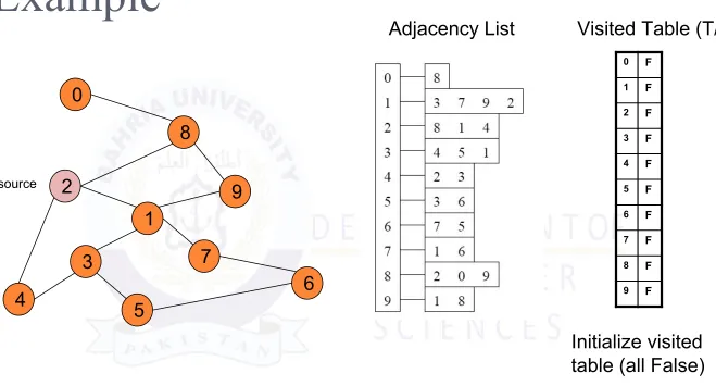
Q = { }

Initialize visited table (all False)

Example

2

4

3

5 1

7

6 9

8 0

Adjacency List

source

0 1 2 3 4 5 6 7 8 9

Visited Table (T/F)

F

F

T

F

F

F

F

F

F

F

Q = { 2 }

Flag that 2 has been visited.

Example

2

4

3

5 1

7

6 9

8 0

Adjacency List

source

0 1 2 3 4 5 6 7 8 9

Visited Table (T/F)

F

T T

F

T

F

F

F

T

F

Q = {2} → { 8, 1, 4 }

Mark neighbors as visited.

Dequeue 2.

Place all unvisited neighbors of 2 on the queue

Example

2

4

3

5 1

7

6 9

8 0

Adjacency List

source

0 1 2 3 4 5 6 7 8 9

Visited Table (T/F)

T T T

F

T

F

F

F

T T

Q = { 8, 1, 4 } → { 1, 4, 0, 9 }

Mark new visited Neighbors.

Dequeue 8.

-- Place all unvisited neighbors of 8 on the queue.

-- Notice that 2 is not placed on the queue again, it has been visited!

Example

2

4

3

5 1

7

6 9

8 0

Adjacency List

source

0 1 2 3 4 5 6 7 8 9

Visited Table (T/F)

T T T T T

F

F

T T T

Q = { 1, 4, 0, 9 } → { 4, 0, 9, 3, 7 }

Mark new visited Neighbors.

Dequeue 1.

-- Place all unvisited neighbors of 1 on the queue. -- Only nodes 3 and 7 haven’t been visited yet.

Example

2

4

3

5 1

7

6 9

8 0

Adjacency List

source

0 1 2 3 4 5 6 7 8 9

Visited Table (T/F)

T T T T T

F

F

T T T

Q = { 4, 0, 9, 3, 7 } → { 0, 9, 3, 7 }

Dequeue 4.

-- 4 has no unvisited neighbors!

Example

2

4

3

5 1

7

6 9

8 0

Adjacency List

source

0 1 2 3 4 5 6 7 8 9

Visited Table (T/F)

T T T T T

F

F

T T T

Q = { 0, 9, 3, 7 } → { 9, 3, 7 }

Dequeue 0.

-- 0 has no unvisited neighbors!

Example

2

4

3

5 1

7

6 9

8 0

Adjacency List

source

0 1 2 3 4 5 6 7 8 9

Visited Table (T/F)

T T T T T

F

F

T T T

Q = { 9, 3, 7 } → { 3, 7 }

Dequeue 9.

-- 9 has no unvisited neighbors!

Example

2

4

3

5 1

7

6 9

8 0

Adjacency List

source

0 1 2 3 4 5 6 7 8 9

Visited Table (T/F)

T T T T T T

F

T T T

Q = { 3, 7 } → { 7, 5 }

Dequeue 3.

-- place neighbor 5 on the queue.

Neighbors

Example

2

4

3

5 1

7

6 9

8 0

Adjacency List

source

0 1 2 3 4 5 6 7 8 9

Visited Table (T/F)

T T T T T T T T T T

Q = { 7, 5 } → { 5, 6 }

Dequeue 7.

-- place neighbor 6 on the queue.

Neighbors

Example

2

4

3

5 1

7

6 9

8 0

Adjacency List

source

0 1 2 3 4 5 6 7 8 9

Visited Table (T/F)

T T T T T T T T T T

Q = { 5, 6} → { 6 }

Dequeue 5.

-- no unvisited neighbors of 5.

Example

2

4

3

5 1

7

6 9

8 0

Adjacency List

source

0 1 2 3 4 5 6 7 8 9

Visited Table (T/F)

T T T T T T T T T T

Q = { 6 } → { }

Dequeue 6.

-- no unvisited neighbors of 6.

Example

2

4

3

5 1

7

6 9

8 0

Adjacency List

source

0 1 2 3 4 5 6 7 8 9

Visited Table (T/F)

T T T T T T T T T T

Q = { } STOP!!! Q is empty!!!

What did we discover?

Look at “visited” tables.

Time Complexity of BFS

(Using adjacency list)

◻

Assume adjacency list

n = number of vertices m = number of edges

Each vertex will enter Q at most once.

Each iteration takes time proportional to deg(v) + 1 (the number 1 is to include the case where deg(v) = 0).

Running time

◻

Given a graph with m edges, what is the total degree?

◻

The total running time of the while loop is:

this is summing over all the iterations in the while loop!

O( Σ

(deg(v)

+

1) )

=

O(n+m)

Time Complexity of BFS

(Using adjacency matrix)

◻

Assume adjacency list

n = number of vertices m = number of edges

Finding the adjacent vertices of v requires checking all elements in the row. This takes linear time O(n).

Summing over all the n iterations, the total running time is O(n2).

O(n

2

)

So, with adjacency matrix, BFS is O(n2) independent of number of edges m. With adjacent lists, BFS is O(n+m); if

Shortest Path Recording

◻

BFS we saw only tells us whether a path exists from source s,

to other vertices v.

It doesn’t tell us the path!

We need to modify the algorithm to record the path.

◻

How can we do that?

Note: we do not know which vertices lie on this path until we reach v!

Efficient solution:

■ Use an additional array pred[0..n-1]

BFS + Path Finding

initialize all pred[v] to -1

Example

Visited Table (T/F)

F F F F F F F F F F

Q = { }

Initialize visited table (all False)

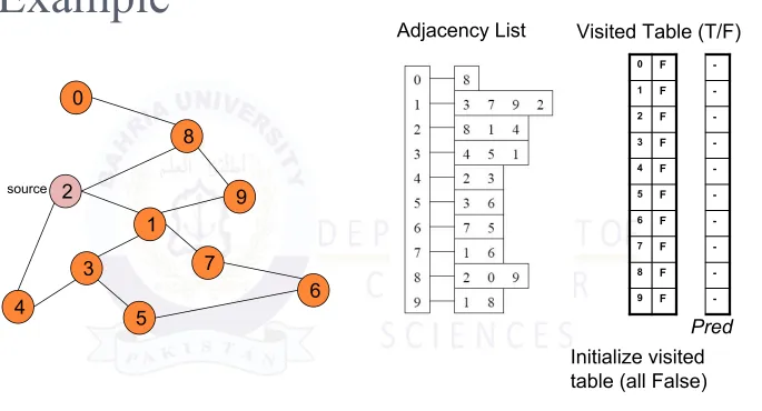
Initialize Pred to -1

Initialize Q to be empty

Example

Visited Table (T/F)

F F T F F F F F F F

Q = { 2 }

Flag that 2 has been visited.

Place source 2 on the queue.

Example

Visited Table (T/F)

F T T F T F F F T F

Q = {2} → { 8, 1, 4 }

Mark neighbors as visited.

Record in Pred that we came from 2.

Dequeue 2.

Place all unvisited neighbors of 2 on the queue

Example

Visited Table (T/F)

T T T F T F F F T T

Q = { 8, 1, 4 } → { 1, 4, 0, 9 }

Mark new visited Neighbors.

Record in Pred that we came from 8.

Dequeue 8.

-- Place all unvisited neighbors of 8 on the queue.

-- Notice that 2 is not placed on the queue again, it has been visited!

Example

Visited Table (T/F)

T T T T T F F T T T

Q = { 1, 4, 0, 9 } → { 4, 0, 9, 3, 7 }

Mark new visited Neighbors.

Record in Pred that we came from 1.

Dequeue 1.

-- Place all unvisited neighbors of 1 on the queue. -- Only nodes 3 and 7 haven’t been visited yet.

Example

Visited Table (T/F)

T T T T T F F T T T

Q = { 4, 0, 9, 3, 7 } → { 0, 9, 3, 7 }

Dequeue 4.

-- 4 has no unvisited neighbors!

Example

2

4

3

5 1

7

6 9

8 0

Adjacency List

source

0 1 2 3 4 5 6 7 8 9

Visited Table (T/F)

T

T

T

T

T

F

F

T

T

T

Q = { 0, 9, 3, 7 } → { 9, 3, 7 }

Dequeue 0.

-- 0 has no unvisited neighbors!

Neighbors 8

2

-1

2

-1

2

8

Example

Visited Table (T/F)

T T T T T F F T T T

Q = { 9, 3, 7 } → { 3, 7 }

Dequeue 9.

-- 9 has no unvisited neighbors!

Example

Visited Table (T/F)

T T T T T T F T T T

Q = { 3, 7 } → { 7, 5 }

Dequeue 3.

-- place neighbor 5 on the queue.

Neighbors

Mark new visited Vertex 5.

Example

Visited Table (T/F)

T T T T T T T T T T

Q = { 7, 5 } → { 5, 6 }

Dequeue 7.

-- place neighbor 6 on the queue.

Neighbors

Mark new visited Vertex 6.

Example

Visited Table (T/F)

T T T T T T T T T T

Q = { 5, 6} → { 6 }

Dequeue 5.

-- no unvisited neighbors of 5.

Example

Visited Table (T/F)

T T T T T T T T T T

Q = { 6 } → { }

Dequeue 6.

-- no unvisited neighbors of 6.

Example

2

4

3

5 1

7

6 9

8 0

Adjacency List

source

0 1 2 3 4 5 6 7 8 9

Visited Table (T/F)

T

T

T

T

T

T

T

T

T

T

Q = { } STOP!!! Q is empty!!!

Pred now can be traced backward to report the path!

8

2

-1

2

3

7

1

2

8

Path reporting

8

2

-1

2

3

7

1

2

8

0 1 2 3 4 5 6 7 8 9

nodes visited from

Try some examples, report path from s to v: Path(0) ->

Path(6) -> Path(1) ->

BFS tree

◻

The paths found by BFS is often drawn as a rooted tree (called BFS tree),

with the starting vertex as the root of the tree.

BFS tree for vertex s=2.

How do we record the shortest

distances?

d(v) = ∞;

Application of BFS

◻

One application concerns how to find

connected components in a graph

◻

If a graph has more than one connected

components, BFS builds a BFS-forest (not just

BFS-tree)!

Conclusion

In this Lecture we discussed…

What are the Depth First & Breadth First Searching?