Research Thesis
In Partial Fulfillment of the
Requirements for the Degree of
Doctor of Philosophy
Tal Mizrahi
Submitted to the Senate of
the Technion - Israel Institute of Technology
Prof. Yoram Moses in the Department of Electrical Engineering
Acknowledgement
I gratefully thank my advisor, Prof. Yoram Moses, for his guidance, support, and encourage-ment throughout my graduate studies. I have been very fortunate to have an advisor who allowed me the freedom to explore on my own, and at the same time provided inspiring guidance that kept me on the right track.
The generous financial assistance of the Technion is gratefully acknowledged.
I would like to gratefully acknowledge the help and support of Marvell.
Many thanks to David Melman for believing in me and giving me the opportunity to pursue my passion.
Many thanks to my parents, Tsipi and Joe, for their encouragement and support.
The results presented in this dissertation have been previously published in:
[1] T. Mizrahi and Y. Moses, “Software defined networks: It’s about time,” in IEEE INFO-COM, 2016.
[2] T. Mizrahi and Y. Moses, “Time4: Time for SDN,” inIEEE Transactions on Network and Service Management (TNSM), under major revision, 2016.
[3] T. Mizrahi and Y. Moses, “OneClock to rule them all: Using time in networked appli-cations,” in IEEE/IFIP Network Operations and Management Symposium (NOMS) mini-conference, 2016.
[4] T. Mizrahi and Y. Moses, “Time capability in NETCONF,” RFC 7758, IETF, 2016.
[5] T. Mizrahi, E. Saat and Y. Moses, “ReversePTP: A clock synchronization scheme for soft-ware defined networks,”International Journal of Network Management (IJNM), accepted, 2016.
[6] T. Mizrahi and Y. Moses, “The Case for Data Plane Timestamping in SDN”, in IEEE INFOCOM Workshop on Software-Driven Flexible and Agile Networking (SWFAN), 2016.
[7] T. Mizrahi, E. Saat and Y. Moses, “Timed consistent network updates in software defined networks,”IEEE/ACM Transactions on Networking (ToN), 2016.
[8] T. Mizrahi, E. Saat and Y. Moses, “Timed consistent network updates,” inACM SIGCOMM Symposium on SDN Research (SOSR), 2015.
[9] T. Mizrahi, O. Rottenstreich and Y. Moses, “TimeFlip: Scheduling network updates with timestamp-based TCAM ranges,” inIEEE INFOCOM, 2015.
[10] T. Mizrahi and Y. Moses, “Using ReversePTP to distribute time in software defined net-works,” inInternational IEEE Symposium on Precision Clock Synchronization for Mea-surement Control and Communication (ISPCS), 2014.
[11] T. Mizrahi and Y. Moses, “ReversePTP: A software defined networking approach to clock synchronization,” inACM SIGCOMM Workshop on Hot topics in Software Defined Net-works (HotSDN), 2014.
[12] T. Mizrahi and Y. Moses, “On the necessity of time-based updates in SDN,” in Open Networking Summit (ONS), 2014.
Abstract 1
List of Abbreviations 3
1 Introduction 5
1.1 Background . . . 5
1.2 Research Goals . . . 6
1.3 Research Methods . . . 7
1.4 Related Work . . . 8
2 TIME4: Time for SDN 11 2.1 abstract . . . 11
2.2 Introduction . . . 12
2.2.1 It’s About Time . . . 12
2.2.2 The Challenge of Dynamic Traffic Engineering in SDN . . . 13
2.2.3 Timed Network Updates . . . 14
2.2.4 Related Work . . . 15
2.2.5 Contributions . . . 17
2.3 The Lossless Flow Allocation (LFA) Problem . . . 18
2.3.1 Inevitable Flow Swaps . . . 18
2.3.2 Model and Definitions . . . 19
2.3.6 n-Swaps . . . 26
2.4 Design and Implementation . . . 29
2.4.1 Protocol Design . . . 29
2.4.2 Prototype Design and Implementation . . . 33
2.5 Evaluation . . . 34
2.5.1 Evaluation Method . . . 34
2.5.2 Performance Attribute Measurement . . . 37
2.5.3 Microbenchmark: Video Swapping . . . 37
2.5.4 Flow Swap Evaluation . . . 39
2.6 Discussion . . . 44
2.7 Conclusion . . . 47
2.8 Acknowledgments . . . 47
3 Timed Consistent Network Updates in SDN 49 3.1 Abstract . . . 49
3.2 Introduction . . . 50
3.2.1 Background . . . 50
3.2.2 Time for Consistent Updates . . . 51
3.2.3 Related Work . . . 52
3.2.4 Contributions . . . 53
3.3 Time-based Consistent Updates . . . 54
3.3.1 Ordered Updates . . . 54
3.3.2 Two-phase Updates . . . 55
3.3.3 k-Phase Consistent Updates . . . 57
3.3.4 The Overhead of Network Updates . . . 57
3.4 Terminology and Notations . . . 57
3.5 Upper and Lower Bounds . . . 60
3.5.1 Delay Upper Bounds . . . 60
3.5.2 Explicit acknowledgment . . . 62
3.5.3 Delay Lower Bounds . . . 63
3.5.4 Scheduling Accuracy Bound . . . 64
3.6 Worst-case Analysis . . . 65
3.6.1 Worst-case Update Duration . . . 65
3.6.2 Worst-case Analysis of Untimed Updates . . . 66
3.6.3 Worst-case Analysis of Timed Updates . . . 69
3.6.4 Timed vs. Untimed Updates . . . 71
3.6.5 Using Acknowledgments . . . 72
3.7 Time as a Consistency Knob . . . 74
3.7.1 An Inconsistency Metric . . . 74
3.7.2 Fine Tuning Consistency . . . 75
3.8 Evaluation . . . 76
3.8.1 Experiment 1: Timed vs. Untimed Updates . . . 77
3.8.2 Experiment 2: Fine Tuning Consistency . . . 79
3.8.3 Simulation: Using ACKs . . . 82
3.9 Discussion . . . 83
3.10 Conclusion . . . 83
4 TIMEFLIP: Scheduling Updates with Timestamp-based TCAM Ranges 85 4.1 Abstract . . . 85
4.2 Introduction . . . 86
4.2.1 Background . . . 86
4.2.2 Introducing TIMEFLIPs . . . 87
4.3.1 Timestamp Format . . . 92
4.3.2 A Path Reroute Scenario . . . 92
4.3.3 The Intuition Behind the Example . . . 94
4.4 Model and Notations . . . 95
4.4.1 TCAM Entries . . . 95
4.4.2 TIMEFLIP: Theory of Operation . . . 96
4.4.3 Timed Installation: Formal Definition . . . 98
4.5 Optimal Time-based Rule Installation . . . 98
4.5.1 Optimal Scheduling . . . 98
4.5.2 Average Expansion . . . 103
4.5.3 Installation Bounds and Periodic Ranges . . . 105
4.5.4 Timestamp Field Size in Bits . . . 108
4.6 Optimal Time-based Action Updates . . . 110
4.7 Experimental Evaluation . . . 113
4.7.1 Simulation-based Evaluation . . . 113
4.7.2 Microbenchmark . . . 115
4.8 Discussion . . . 119
4.8.1 Scheduling Accuracy . . . 119
4.8.2 Timestamp Size in Real-Life . . . 120
4.8.3 TCAM Update Performance . . . 120
4.8.4 Timed Updates of Non-TCAM Memories . . . 121
4.8.5 On the TCAM Encoding Scheme . . . 121
4.9 Conclusion . . . 123
5 OneClock to Rule Them All: Using Time in Networked Applications 125 5.1 Abstract . . . 125
5.2.3 OneClock: Accurate Scheduling . . . 127
5.2.4 Related Work . . . 128
5.2.5 Contributions . . . 129
5.3 Using OneClock in Practice . . . 130
5.3.1 Coordinated Operation . . . 130
5.3.2 Coordinated Snapshot . . . 130
5.3.3 Network-wide Atomic Commit . . . 131
5.4 NETCONF Time Extension . . . 133
5.4.1 Overview . . . 133
5.4.2 Applying the Time Primitives to Various Applications . . . 134
5.4.3 Notifications and Cancellation Messages . . . 134
5.4.4 Clock Synchronization . . . 135
5.4.5 Acceptable Scheduling Range . . . 135
5.5 Prediction-based Scheduling . . . 136
5.5.1 ETE Measurements . . . 137
5.5.2 ETE Prediction Algorithms . . . 137
5.6 Evaluation . . . 141
5.6.1 Background . . . 141
5.6.2 Experiment I: Performance on different platforms . . . 142
5.6.3 Experiment II: Periodic vs. bursty measurement . . . 143
5.6.4 Experiment III: Performance under synthetic workload . . . 143
5.7 Discussion . . . 144
5.8 Conclusion . . . 146
5.9 Acknowledgments . . . 146
6.2.2 REVERSEPTP in a Nutshell . . . 150
6.2.3 Related Work . . . 151
6.2.4 Contributions . . . 152
6.3 Preliminaries . . . 152
6.3.1 A Brief Overview of PTP . . . 152
6.3.2 A Model for using Time in SDN . . . 154
6.4 REVERSEPTP: Theory of Operation . . . 155
6.5 The REVERSEPTP Profile . . . 159
6.6 Using REVERSEPTP in SDNs . . . 162
6.6.1 The REVERSEPTP Architecture in SDN . . . 162
6.6.2 Time-based Updates using REVERSEPTP . . . 164
6.6.3 Time Distribution over SDNs using REVERSEPTP . . . 165
6.7 Evaluation . . . 166
6.7.1 Time-triggered Events . . . 167
6.7.2 Scalability . . . 170
6.8 Discussion . . . 172
6.8.1 Accuracy . . . 172
6.8.2 Scalability-Programmability Tradeoff . . . 172
6.8.3 Synchronizing Clocks using REVERSEPTP . . . 173
6.8.4 REVERSEPTP in an SDN with Multiple Controllers . . . 173
6.8.5 Security aspects . . . 174
6.9 Conclusion . . . 174
7 Conclusion 177 7.1 Summary of Results . . . 177
2.1 Flow Swapping—Flows need to convert from the “before” configuration to the
“after”. . . 14
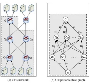
2.2 Modeling a Clos topology as an unsplittable flow graph. . . 18
2.3 The LFA game: the source’s procedure. . . 22
2.4 The LFA game: the controller’s procedure. . . 22
2.5 AScheduled Bundle: theBundle Commitmessage may includeTs, the scheduled time of execution. The controller can use a Bundle Discard message to cancel theScheduled Bundlebefore timeTs. . . 31
2.6 REVERSEPTP in SDN: switches distribute their time to the controller. Switches’ clocks are not synchronized. For every switch i, the controller knows offseti between switchi’s clock and its local clock. . . 32
2.7 TIME4 prototype design: the black blocks are the components implemented in the context of this work. . . 33
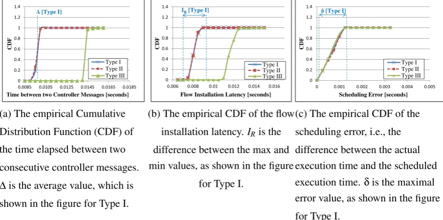
2.8 Measurement of the three performance attributes: (a)∆, (b)IR, and (c)δ. . . 36
2.9 Microbenchmark: video swapping. . . 38
than SWAN and B4 (b), while the latter two methods incur higher overhead.
Combining TIME4 with SWAN or B4 provides the best of both worlds; low
packet loss (b) and low overhead (c and d). . . 41
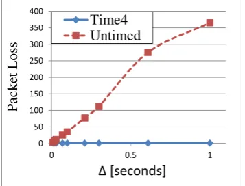
2.12 The number of packets lost in a flow swap vs. ∆. The packet loss in TIME4 is not affected by the controller’s performance (∆). . . 43
2.13 Performance as a function of IR and δ. Untimed updates are affected by the installation latency variation (IR), whereas TIME4 is affected by the scheduling error (δ). TIME4 is advantageous since typicallyδ<IR. . . 43
3.1 Update procedure examples. . . 54
3.2 Ordered update procedure for the scenario of Fig. 3.1a. . . 55
3.3 Timed Ordered update procedure for the scenario of Fig. 3.1a. . . 55
3.4 Two-phase update procedure for the scenario of Fig. 3.1b. . . 56
3.5 Timed two-phase update procedure for the scenario of Fig. 3.1b. . . 56
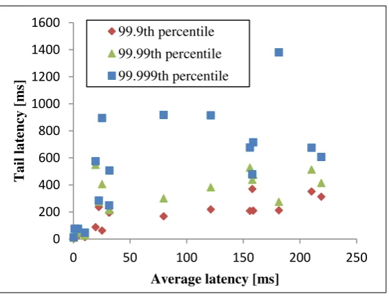
3.6 Long-tail latency . . . 62
3.7 A PERT chart of ak-phase update. . . 66
3.8 A PERT chart of a two-phase update with garbage collection, performed after phase 2 is completed. Garbage collection removes the ‘before’ configuration (see Fig. 3.1) from the switches that took part in phase 1. . . 68
3.9 A PERT chart of a timed two-phase update with garbage collection. . . 70
3.10 PERT charts of the garbage collection phase of an ACK-based update. . . 73
3.11 Example 3.16: PERT chart of a timed two-phase update. The delayd(red in the figure) is a knob for consistency. . . 76
3.12 Leaf-spine topology. . . 77
OpenFlow switches. White nodes represent the external source and destination
of the test flows in the experiment. . . 80
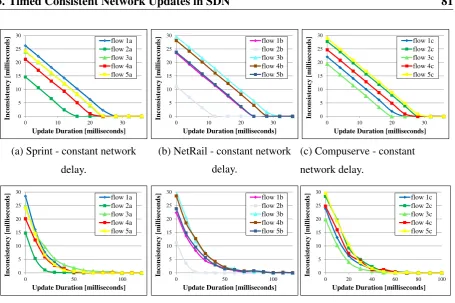
3.15 Inconsistency as a function of the update duration. Modifying the update dura-tion controls the degree of inconsistency. Two graphs are shown for each of the three topologies: exponential delay, constant delay. . . 81
3.16 Update duration of the garbage collection phase. . . 82
4.1 TCAM lookup: conventional vs. TIMEFLIP. TIMEFLIPuses a timestamp field, representing the time rangeT ≥T0. . . 87
4.2 Scheduling tolerance: T0∈[Tmin,Tmax]. . . 89
4.3 Time range examples. . . 92
4.4 Flows need to convert from the ‘before’ configuration to the ‘after’. . . 93
4.5 Scheduling timelines. . . 93
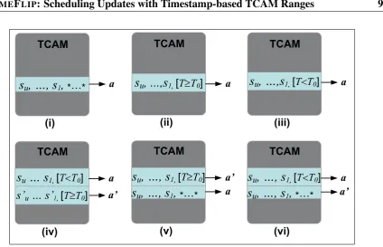
4.6 A timed TCAM Update. Every line in the figure is a time range rule, repre-sented by one or more TCAM entries. (i) Time-oblivious entry. (ii) Installation. (iii) Removal. (iv) Rule update. (v) Action update. (vi) Action update using a complementary timestamp range. . . 97
4.7 Optimal scheduling algorithm; no other scheduling algorithm produces an ex-tremal range with a lower expansion. . . 101
4.8 Installation bounds . . . 106
4.9 Periodic ranges: the 2V-periodic continuation of[T0,T1]. (i) ForT1V->T0V-. (ii) ForT1V-<T0V-. In BOUNDEDRANGET1=T0+2V−1−1. . . 106
4.10 Determining a range with installation bounds∆. . . 107
4.11 Example of 1-bit timestamp, per Theorem 4.13. . . 109
4.12 Algorithm for finding reduced range with installation bounds. . . 112
4.13 REDUCEDRANGE: proof of Lemma 4.17. . . 113
4.16 The number of bits as a function of∆for various values of , using BOUND
-EDRANGE in a timed installation. The star-shaped markers indicate the points
whereTOL=2dlog2(∆)e. . . 116
4.17 Timed action updates: REDUCEDRANGE vs. BOUNDEDRANGE. . . 116
4.18 Microbenchmark . . . 117
4.19 Timed updates in non-TCAM lookups . . . 122
5.1 Elapsed Time of Execution (ETE): ETE =Te−Ts. . . 128
5.2 Prediction-based scheduling: by predicting the ETE, a client can control when the RPC will becompleted. . . 129
5.3 Coordinated operations and coordinated snapshots. . . 131
5.4 The time capability in NETCONF. . . 132
5.5 Atomic commit: (a) NETCONF confirmed commit, without using time. (b) Time-triggered commit. . . 132
5.6 Cancellation message. . . 135
5.7 Acceptable scheduling range: defined by two configurable parameters: sched-max-future and sched-max-past. . . 136
5.8 Prediction-based scheduling approach. . . 137
5.9 Performance on various machine types (a). Type V machines were used in (b) and (c). . . 141
5.10 Instantaneous prediction error viewed over a 150 second period. The behavior shows peaks under synthetic workload. (a) was measured on Azure, and (b), (c) on Type V machines. . . 142
6.1 Time distribution in PTP and REVERSEPTP. . . 150
6.2 The Precision Time Protocol (PTP). . . 153
6.3 A protocol for coordinated network updates. . . 155
SDN that runs conventional PTP, a typical approach would be for the controller
to run a PTP master, and for each switch to be a PTP slave. . . 163
6.6 Coordinated updates using REVERSEPTP. . . 164
6.7 SDN as a Boundary Clock. . . 166
6.8 Network setup. . . 168
6.9 Accuracy measurements of a coordinatedPing. The timestamped event experi-ment (b) provides a rough estimate of the clock accuracy. . . 169
6.10 REVERSEPTP vs. PTP: rate of PTP messages sent or received by each node. . . 170
6.11 CPU Utilization in REVERSEPTP and in PTP as a function of the number of nodes. The figures are presented for two machines types: Type I is a low perfor-mance machine, and Type II is high perforperfor-mance. . . 171
This dissertation analyzes the use of accurate time to coordinate network configuration updates.
Specifically, this work focuses on centralized network architectures, such as Software Defined
Networks (SDN).
Time can be beneficial in a wide variety of network update scenarios. The current work
focuses on two key scenarios in which using time has a significant advantage over
state-of-the-art approaches. First, we characterize a set of update scenarios called flow swaps, for which
timed updates are the optimal update approach, yielding less packet loss than existing update
approaches. Second, we analyze the use of accurate time to schedule multi-phase update
pro-cedures, allowing updates to be performed consistently, while requiring less resource overhead
than existing network update methods.
The current work also introduces a clock synchronization scheme that is adapted to the
centralized SDN environment. However, even if network devices have perfectly synchronized
clocks, how can we guarantee that events are executed at the exact time for which they were
scheduled? In this work we present and analyze two accurate scheduling methods. The first
uses Ternary Content Addressable Memory (TCAM) ranges in hardware switches. The second
is a prediction-based scheduling approach that uses timing information collected at runtime to
accurately schedule future operations. Both methods are shown to be practical and efficient.
Finally, this thesis defines extensions to standard network protocols, enabling practical
im-plementations of our concepts. We define a new feature in OpenFlow called Scheduled Bundles,
which has been incorporated into the OpenFlow 1.5 protocol. A similar capability was defined
for the NETCONF protocol, and has been published as an RFC.
ACK Acknowledgment
ETE Elapsed Time of Execution
Gbps Gigabits per second
IETF Internet Engineering Task Force
IoT Internet of Things
LFA Lossless Flow Allocation
Mbps Megabits per second
MEF Metro Ethernet Forum
NETCONF Network Configuration Protocol
NFV Network Function Virtualization
NTP Network Time Protocol
ONF Open Networking Foundation
PERT Program Evaluation and Review Technique
PTP Precision Time Protocol
RPC Remote Procedure Call
SDN Software Defined Networking
SNMP Simple Network Management Protocol
TOL Scheduling Tolerance
VM Virtual Machine
VNF Virtual Network Function
Introduction
1.1
Background
The use of synchronized clocks was first introduced in the 19th century by the Great Western
Railway company in Great Britain. Clock synchronization has significantly evolved since then,
and is now a mature technology that is being used by various different applications, from mobile
backhaul networks [15] to distributed databases [16].
Network configuration updates are a routine necessity, and must be performed in a way that
minimizes transient effects caused by intermediate states of the network. This challenge is
espe-cially critical in the context of Software Defined Networks, where the control plane is managed
by a logically centralizedcontroller, which frequently sends configuration updates to the network
switches. These updates modify the switches’ forwarding rules, and thus directly affect how
packets are forwarded through the network. The controller must take care to minimize network
anomalies during update procedures, such as packet drops or misroutes caused by temporary
in-consistencies. Updates must also be planned with performance in mind; update procedures must
scale with the size of the network, and thus cannot be too complex.
The current work analyzes the use of clocks and time as a tool in network reconfiguration.
While the notion of using time to trigger events in distributed systems is certainly not new (e.g.,
[17]), time-based triggers were typically considered impractical in the context of network
man-agement due to the inaccuracy of network time synchronization. Prior to the current work,
as SNMP [19] and NETCONF [20], made use of accurate time for scheduling or
coordinat-ing configuration updates. However, network clock synchronization has evolved over the last
few years. The Precision Time Protocol (PTP), defined in the IEEE 1588 standard [21], can
synchronize clocks in a network to a very high degree of accuracy, typically on the order of
mi-croseconds. Moreover, in the last few years PTP has become a common feature in commodity
network devices. Thus, accurate time appears to be an accessible and useful tool for coordinating
configuration changes.
1.2
Research Goals
In this thesis we study the use of time in centralized network environments, with an emphasis on
SDN. Specifically, four aspects of this problem are analyzed.
Use cases that benefit from using time. A key goal of our research is to identify and analyze network scenarios in which a time-based approach is useful and beneficial. We start
by analyzing TIME4 (Chapter 2), which is an update approach that performs multiple changes
at different switches at the same time. We then study timed multi-phase updates, where each
phase is scheduled to be performed at a different execution time (Chapter 3). We then consider
the use of time as a generic approach that can be applied not only to switches and routers, but
to any managed device: sensors, actuators, Internet of Things (IoT) devices, routers, or toasters
(Chapter 5).
Network protocols. One of the goals of this work is to extend standard network configura-tion protocols with the ability to use time-triggered operaconfigura-tions. These extensions are defined for
OpenFlow (Chapter 2), and for NETCONF (Chapter 5).
Accurate scheduling methods. Even if network devices have perfectly synchronized clocks, it is potentially challenging to guarantee that updates are performed at the exact time for which
they were scheduled; a scheduling mechanism that relies on the switch’s software may be
af-fected by the switch’s operating system and by other running tasks. The current work analyzes
scheduling methods that allow a high degree of accuracy. Specifically, two methods are
switches (Chapter 4), and (ii) a prediction-based scheduling approach that uses timing
informa-tion collected at runtime to accurately schedule future operainforma-tions (Chapter 5).
Clock synchronization in SDN. Accurate timekeeping requires a clock synchronization method, such as the Precision Time Protocol (PTP) [21]. Contrary to the centralized SDN
paradigm, PTP is by nature a decentralized protocol, in which every node is required to run
complex algorithmic logic. In this work we explore a clock synchronization scheme that is
adapted to the centralized SDN environment (Chapter 6).
1.3
Research Methods
The research described in this dissertation involves several methods and disciplines, both
theo-retical and experimental.
Theoretical tools. The study of flow swapping (Chapter 2) uses a game theoretic analysis in the context of network flow problems. The analysis of timed consistent updates (Chapter 3)
uses the network update abstraction of [22], and analyzes the worst-case duration of network
updates, including the use of Program Evaluation and Review Technique (PERT) graphs [23].
Timestamp-based TCAM ranges (Chapter 4) are studied using a combinatorial approach; we
present algorithms that minimize the number of TCAM entries and the number of bits used to
represent a timestamp range in a TCAM. The work on OneClock (Chapter 5) uses a time-series
analysis; periodic measurements of the execution time of a Remote Procedure Call (RPC) are
used to predict the next execution time.
Network protocols. This research work defines extensions to standard network protocols; a time extension to OpenFlow (Chapter 2), and a similar extension to NETCONF (Chapter 5). In
order to pursue these extensions we actively participated in the two standard organizations that
define these protocols, the Open Networking Foundation (ONF), and the Internet Engineering
Task Force (IETF). Open source prototypes were implemented for the two extensions, and these
prototypes were used in our experimental evaluation.
performed using two academic testbeds, Emulab [24] and DeterLab [25]. The experiments were
run over a large number of nodes, up to 70 in some of the experiments. The experiments allowed
an emulated network environment, where each node ran one of our time-enabled prototypes.
Various network topologies were used, including well-known publicly available topologies [14].
Public cloud networks were also used for some of the experiments (Chapter 5), namely Amazon’s
AWS and Microsoft’s Azure. Some of the analysis was assisted by simulation-based evaluation
(Chapters 3 and 4). In the context of timestamp-based TCAM ranges (Chapter 4), the
eval-uation also included an experiment on a real-life network switch. Publicly available real-life
measurements [26, 27] were also used in some of the analysis (Chapter 3).
1.4
Related Work
Consistent network updates. A network configuration update is per-packet consistent [22] if it guarantees that every packet sent through the network is processed according to a single
configuration version, either the previous or the current one. A common approach to avoiding
inconsistencies that may result from configuration updates is to use a sequence of
configura-tion commands (e.g., [28, 29, 30, 31, 32]), whereby the order of execuconfigura-tion guarantees that no
anomalies are caused in intermediate states of the procedure. Thissequential approachis fairly
complex, as it requires the SDN programmer to carefully consider all intermediate states, and
to find a successful sequence of commands. Moreover, since this approach requires updates to
take place in a specific order, the controller uses a series of request-acknowledge handshakes,
yielding a long execution time. Moreover, the efficiency of the update process is very sensitive
to the load and specific conditions at runtime. Thus, while this sequential approach guarantees
consistency, it is costly in terms of performance.
Another approach for consistent updates [22] uses configuration version tags to guarantee
consistency; all packets are stamped with a configuration version tag that indicates whether they
should be processed by the new configuration or the old one, in order to guarantee that each
packet is processed by a single configuration at all switches along its path. Thisversion-based
perspec-tive, but is still complex in terms of the number of messages exchanged between the controller
and switches. Moreover, this approach implies that during intermediate states of the update
switches must maintain the configurations of both the previous and the current configuration,
thus consuming costly memory space in the switch, as discussed in [33].
Using time in distributed applications. The use of time in distributed applications has been widely analyzed, both in theory and in practice. Analysis of the usage of time and synchronized
clocks, e.g., Lamport [34, 17] dates back to the late 1970s and early 1980s. In recent years, as
accurate time has become an accessible and affordable tool, it is used in various different
applica-tions; Google’s Spanner [16] uses synchronized clocks as a tool for synchronizing a distributed
database. Industrial automation systems [35] use synchronized clocks to allow deterministic
response times of machines to external events, and to enforce coordinated orchestration in a
factory product line. The Time Sensitive Networking (TSN) technology [36] is used in
automo-tive networks and in audio/video streaming applications. The well-known particle accelerators
at CERN use state-of-the-art clock synchronization [37], allowing sub-nanosecond accuracy in
response to management messages that control the accelerator experiments. While the usage of
accurate time in distributed systems has been widely discussed in the literature, we are not aware
of similar analyses of the usage of accurate time as a means for performing accurately scheduled
configuration updates in computer networks.
Using time in computer networks. Time is used in networks to schedule events at a coarse resolution. Periodic backups and power-save policies are often invoked at a scheduled
time-of-day. Time-of-day routing[38, 39] routes traffic to different destinations based on the time-of-day.
Such updates are typically performed at a low rate and do not place demanding requirements on
consistency or performance. Hence, time-of-day routing does not require the usage ofaccurate
time; a time accuracy on the order of seconds is typically more than enough for this purpose.
In [40] the authors briefly mentioned that it would be interesting to explore the use of time
synchronization to instruct routers or switches to change from one configuration to another at a
specific time, but did not pursue the idea beyond this observation.
of traffic flows is monitored by measuring and logging the start-time and end-time of flows in
the network. OpenFlow also usestimeoutsfor expiring old forwarding rules; the controller can
define a timeout for a flow rule, causing it to be removed when the timeout expires. However,
timeouts are defined in OpenFlow as a means to age out unused rules, and not as a means to
schedule configuration updates, and are therefore defined with a coarse granularity of 1 second.
Prior to the current work, neither the OpenFlow protocol [18, 42] nor common management
and configuration protocols, such as SNMP [19] and NETCONF [20], used accurate time for
T
IME
4: Time for SDN
This chapter is a preprinted version of the paper:
[2] T. Mizrahi and Y. Moses, “Time4: Time for SDN,” inIEEE Transactions on Network and
Service Management (TNSM), under major revision, 2016.
An early version of this paper was published in IEEE INFOCOM 2016 [1]. Preliminary
versions of this work were published as short papers, one in HotSDN 2013 [13], and the other in
the Open Networking Summit (ONS) 2014 [12].
2.1
abstract
With the rise of Software Defined Networks (SDN), there is growing interest in dynamic and
centralized traffic engineering, where decisions about forwarding paths are taken dynamically
from a network-wide perspective. Frequent path reconfiguration can significantly improve the
network performance, but should be handled with care, so as to minimize disruptions that may
occur during network updates.
Network updates are especially challenging when the network is heavily utilized; some of
the existing approaches suggest that spare capacity should be reserved in the network in order to
allow updates in such scenarios, or that the network load should be temporarily reduced prior to
In this paper we introduce TIME4, an approach that uses accurate time to coordinate network
updates. TIME4 is a powerful tool in softwarized environments, that can be used for various
network update scenarios, including in heavily utilized networks. Specifically, we characterize
a set of update scenarios called flow swaps, for which TIME4 is the optimal update approach,
yielding less packet loss than existing update approaches without requiring spare capacity, and
without temporarily reducing the network’s bandwidth. We define the lossless flow allocation
problem, and formally show that in environments with frequent path allocation, scenarios that
require simultaneous changes at multiple network devices are inevitable.
We present the design, implementation, and evaluation of a TIME4-enabled OpenFlow
pro-totype. The prototype is publicly available as open source. Our work includes an extension to
the OpenFlow protocol that has been adopted by the Open Networking Foundation (ONF), and
is now included in OpenFlow 1.5. Our experimental results show the significant advantages of
TIME4 compared to other network update approaches, and demonstrate an SDN use case that is
infeasible without TIME4.
2.2
Introduction
2.2.1
It’s About Time
The use of synchronized clocks was first introduced in the 19th century by the Great Western
Railway company in Great Britain. Clock synchronization has significantly evolved since then,
and is now a mature technology that is being used by various different applications, including
MBH (Mobile Backhaul) networks [15], industrial automation systems [35], power grid
net-works [43] and distributed databases [16].
The Precision Time Protocol (PTP), defined in the IEEE 1588 standard [21], can synchronize
clocks to a very high degree of accuracy, typically on the order of 1 microsecond [44, 15, 45].
PTP is a common and affordable feature in commodity switches. Notably, 9 out of the 13
SDN-capable switch silicons listed in the Open Networking Foundation (ONF) SDN Product
Direc-tory [46] have native IEEE 1588 support [47, 48, 49, 50, 51, 52, 53, 54, 55].
and clock synchronization, it is only natural to harness this powerful technology to coordinate
events in SDNs.
2.2.2
The Challenge of Dynamic Traffic Engineering in SDN
Defining network routes dynamically, based on a complete view of the network, can significantly
improve the network performance compared to the use of distributed routing protocols. SDN and
OpenFlow [41, 18] have been leading trends in this context, but several other ongoing efforts
offer similar concepts. The Interface to the Routing System (I2RS) working group [56], and the
Forwarding and Control Element Separation (ForCES) working group [57] are two examples of
such ongoing efforts in the Internet Engineering Task Force (IETF).
Centralized network updates, whether they are related to network topology, security policy,
or other configuration attributes, often involve multiple network devices. Hence, updates must
be performed in a way that strives to minimize temporary anomalies such as traffic loops,
con-gestion, or disruptions, which may occur during transient states where the network has been
partially updated.
While SDN was originally considered in the context of campus networks [41] and data
cen-ters [58], it is now also being considered for Wide Area Networks (WANs) [33, 59], carrier
networks, and MBH (Mobile Backhaul) networks [60].
WAN and carrier-grade networks require a very low packet loss rate. Carrier-grade
perfor-mance is often associated with the termfive nines, representing an availability of 99.999%. MBH
networks require a Frame Loss Ratio (FLR) of no more than 10−4for voice and video traffic, and no more than 10−3 for lower priority traffic [61]. Other types of carrier network applications, such as storage and financial trading require even lower loss rates [62], on the order of 10−5.
Several recent works have explored the realm of dynamic path reconfiguration, with frequent
updates on the order of minutes [33, 59, 30], enabled by SDN. Interestingly, for voice and video
traffic, a frame loss ratio of up to 10−4implies that service must not be disrupted for more than 6 milliseconds per minute. Hence, if path updates occur on a per-minute basis, then transient
2.2.3
Timed Network Updates
We explore the use ofaccurate timeas a tool for performing coordinated network updates in a
way that minimizes packet loss. Softwarized management can significantly benefit from using
time for coordinating network-wide orchestration, and for enforcing a given order of events.
We introduce TIME4, which is an update approach that performs multiple changes at different
switches at the same time.
Example 2.1. Fig. 2.1 illustrates a flow swapping scenario. In this scenario, the forwarding paths of two flows, f1and f2, need to be reconfigured, as illustrated in the figure. It is assumed
that all links in the network have an identical capacity of 1 unit, and that both f1 and f2require
a bandwidth of 1 unit. In the presence of accurate clocks, by scheduling S1and S3to update their
paths at the same time, there is no congestion during the update procedure, and the
reconfigu-ration is smooth. As clocks will typically be reasonably well synchronized, albeit not perfectly
synchronized, such a scheme will result in a very short period of congestion.
S
1S
2S
3S
4
S
5f
1f
2S
1S
2S
3S
4
S
5f
1f
2before
after
Figure 2.1: Flow Swapping—Flows need to convert from the “before” configuration to the “after”.
In this paper we show that in a dynamic environment, where flows are frequently added,
removed or rerouted, flow swaps are inevitable.
One of our key results is that simultaneous updates are the optimal approach in scenarios such
as Example 1, whereas other update approaches may yield considerable packet loss, or incur
higher resource overhead. Note that such packet loss can be reduced either by increasing the
capacity of the communication links, or by increasing the buffer memories in the switches. We
The importance of flow swaps. The necessity of flow swapping is not confined to the spe-cific example of Fig. 2.1. More generally, in some update scenarios, known asdeadlocks[30], it has been shown that it is not possible to complete the update without incurring congestion.
Simultaneous flow swapping is generally applicable to all deadlock scenarios.
The need to rearrange flows in heavily utilized networks was discussed both in SWAN [33]
and in B4 [59]. As we show in this paper, timed flow swapping can address the scenarios of
SWAN and B4 without requiring extra network capacity, and without temporarily reducing the
traffic bandwidth.
Another notable example of the importance of flow swaps is a recently published work by
Fox Networks [63], in which accurately timed flow swaps are essential in the context of video
switching.
Accuracyis a key requirement in TIME4; since updates cannot be applied at the exact same
instant at all switches, they are performed within a short time interval called the scheduling
error. This error is affected by two factors: (i) the clock accuracy, and (ii) the switch’s ability
to execute the update as close as possible to its scheduled time. The switches’ clocks can be
synchronized in typical systems with a sub-microsecond accuracy (e.g., [44]). As for factor (ii),
the latency of rule installations has been shown to range from milliseconds to seconds [64, 30]. In
contrast,timedupdates, using the TCAM-based hardware solution ofTimeFlip [9], have been shown to allow a sub-microsecond scheduling error. The experiments we present in Section 2.5
show that the scheduling error insoftware switches is on the order of 1 millisecond. Accurate
hardware-based solutions such as TimeFlip can execute scheduled events in existing switches with an accuracyon the order of 1 microsecond.
Accurate time is a powerful abstraction for SDN programmers, not only for flow swaps, but
also fortimed consistent updates, as discussed by [8].
2.2.4
Related Work
Time and synchronized clocks have been used in various distributed applications, e.g., [15, 35,
time-of-day. Path calendaring [65] can be used to configure network paths based on scheduled or foreseen
traffic changes. The two latter examples are typically performed at a low rate and do not place
demanding requirements on accuracy.
Various network update approaches have been analyzed in the literature. A common
ap-proach is to use a sequence of configuration commands [28, 31, 32, 30], whereby the order
of execution guarantees that no anomalies are caused in intermediate states of the procedure.
However, as observed by [30], in some update scenarios, known asdeadlocks, there is no order that guarantees a consistent transition.Two-phaseupdates [22] use configuration version tags to
guarantee consistency during updates. However, as per [22], two-phaseupdates cannot
guaran-tee congestion freedom, and are therefore not effective in flow swap scenarios, such as Fig. 2.1.
Hence, in flow swap scenarios theorderapproach and thetwo-phaseapproach produce the same
result as the simple-minded approach, in which the controller sends the update commands as
close as possible to instantaneously, and hopes for the best.
In this paper we present TIME4, an update approach that is most effective in flow swaps and
other deadlock [30] scenarios, such as Fig. 2.1. We refer to update approaches that do not use
time asuntimedupdate approaches.
In SWAN [33], the authors suggest that reserving unused scratch capacity of 10-30% on
every link can allow congestion-free updates in most scenarios. The B4 [59] approach prevents
packet loss during path updates by temporarily reducing the bandwidth of some or all of the
flows. Our approach does not require scratch capacity, and does not reduce the bandwidth of
flows during network updates. Furthermore, in this paper we show that variants of SWAN and
B4 that make use of TIME4 can perform better than the original versions.
A recently published work by Fox Networks [63] shows that accurately timed path updates
are essential for video swapping. We analyze this use case further in Section 2.5.
Rearrangeably non-blocking topologies (e.g., [66]) allow new traffic flows to be added to the
network by rearranging existing flows. The analysis of flow swaps presented in this paper
em-phasizes the requirement to performsimultaneousreroutes during the rearrangement procedure,
an aspect which has not been previously studied.
time in SDN [13] and the flow swapping scenario [12]. The use of time forconsistent updates
was discussed in [8]. TimeFlip [9] presented a practical method of implementing timed updates.
The current work is the first to present a generic protocol for performing timed updates in SDN,
and the first to analyzeflow swaps, a natural application in which timed updates are the optimal
update approach.
2.2.5
Contributions
The main contributions of this paper are as follows:
• We consider a class of network update scenarios calledflow swaps, and show that
simul-taneous updates using synchronized clocks are provably the optimal approach of
imple-menting them. In contrast, existing approaches for consistent updates (e.g., [22, 30]) are
not applicable to flow swaps, and other update approaches such as SWAN [33] and B4 [59]
can perform flow swaps, but at the expense of increased resource overhead.
• We use game-theoretic analysis to show that flow swaps are inevitable in the dynamic
nature of SDN.
• We present the design, implementation and evaluation of a prototype that performs timed
updates in OpenFlow.
• Our work includes an extension to the OpenFlow protocol that has been approved by the
ONF and integrated into OpenFlow 1.5 [67], and into the OpenFlow 1.3.x extension
pack-age [68]. The source code of our prototype is publicly available [69].
• We present experimental results that demonstrate the advantage of timed updates over
existing approaches. Moreover, we show that existing update approaches (SWAN and B4)
can be improved by using accurate time.
• Our experiments include an emulation of an SDN-controlled video swapping scenario,
a real-life use case that has been shown [63] to be infeasible with previous versions of
d
q1 q2
o1 o2
(a) Clos network.
d
o1 o2 on
q1 q2 qm
c c c
s ∞
∞ ∞
c c c
e1 e2 em
(b) Unsplittable flow graph.
Figure 2.2: Modeling a Clos topology as an unsplittable flow graph.
2.3
The Lossless Flow Allocation (LFA) Problem
2.3.1
Inevitable Flow Swaps
Fig. 2.1 presents a scenario in which it is necessary toswaptwo flows, i.e., to update two switches
at the same time. In this section we discuss the inevitability of flow swaps; we show that there
does not exist a controller routing strategy that avoids the need for flow swaps.
Our analysis is based on representing the flow-swap problem as an instance of an unsplittable
flow problem, as illustrated in Fig. 2.2b. The topology of the graph in Fig. 2.2b models the traffic
behavior to a given destination in common multi-rooted network topologies such as fat-tree and
Clos (Fig. 2.2a).
The unsplittable flow problem [70] has been thoroughly discussed in the literature; given a
directed graph, a source nodes, a destination noded, and a set of flow demands (commodities)
this paper we define a gamebetween two players: asource1 that generates traffic flows (com-modities) and a controllerthat reconfigures the network forwarding rules in a way that allows the network to forward all traffic generated by the source without packet losses.
Our main argument, phrased in Theorem 2.2, is that the source has a strategy thatforcesthe controller to perform a flow swap, i.e., to reconfigure the path of two or more flows at the same
time. Thus, a scenario in which multiple flows must be updated at thesame timeis inevitable, implying the importance of timed updates.
Moreover, we show that the controller can be forced to invoken individual commands that
should optimally be performed at the same time. Update approaches that do not use time, also
known asuntimedapproaches, cause the updates to be performed over a long period of time, po-tentially resulting in slow and possibly erratic response times and significant packet loss. Timed
coordination allows us to perform thenupdates within a short time interval that depends on the
scheduling error.
Although our analysis focuses on the topology of Fig.2.2b, it can be shown that the results
are applicable to other topologies as well, where the source can force the controller to perform a
swap over the edges of the min-cut of the graph.
2.3.2
Model and Definitions
We now introduce thelossless flow allocation (LFA)problem; it is not presented as an
optimiza-tion problem, but rather as a game between two players: a source and a controller. As the source adds or removes flows (commodities), the controller reconfigures the forwarding rules
so as to guarantee that all flows are forwarded without packet loss. The controller’s goalis to find a forwarding path for all the flows in the system without exceeding the capacity of any of
the edges, i.e., to completely avoid loss of packets from the given flows. The source’s goalis to progressively add flows, without exceeding the network’s capacity, forcing the controller to
perform a flow swap. We shall show that the source has a strategy that forces the controller to
1The source player does not represent a malicious attacker; it is an ‘adversary’, representing the worst-case
swap traffic flows simultaneously in order to avoid packet loss.
Our model makes three basic assumptions: (i) each flow has a fixed bandwidth, (ii) the controller strives to avoid packet loss, and (iii) flows are unsplittable. We discuss these as-sumptions further in Sec. 2.6.
The term flow in classic flow problems typically refers to the amount of traffic that is
for-warded through each edge of the graph. Since our analysis focuses on SDN, we slightly divert
from the common flow problem terminology, and use the termflowin its OpenFlow sense, i.e., a
set of packets that share common properties, such as source and destination network addresses.
A flow in our context, can be seen as a session between the source and destination that runs
traffic at a fixed rate.
The network is represented by a directed weighted acyclic graph (Fig. 2.2b),G= (V,E,c), with a sources, a destinationd, and a set of intermediate nodes,Vin. Thus,V=Vin∪ {s,d}. The nodes directly connected to sare denoted by O={o1,o2, . . . ,on}. Each of the outgoing edges from the sourceshas an infinite capacity, whereas the rest of the edges have a capacityc. For the
sake of simplicity, and without loss of generality, throughout this section we assume thatc=1.
Such a graphGis referred to as anLFA graph.
The source node progressively transmits traffic flows towards the destination node. Each flow
represents a session betweensandd; every flow has a constant bandwidth, and cannot be split
between two paths. A centralized controller configures the forwarding policy of the intermediate
nodes, determining the path of each flow. Given a set of flows fromstod, the controller’s goal
is to configure the forwarding policy of the nodes in a way that allows all flows to be forwarded
todwithout exceeding the capacity of any of the edges.
The set of flows that are generated bysis denoted byF::={F1,F2, . . . ,Fk}. Each flowFi is defined asFi::= (i,fi,ri), whereiis a unique flow index, fiis the bandwidth satisfying 0< fi≤c, andridenotes the node that the controller forwards the flow to, i.e.,ri∈ {o1,o2, . . . ,on}.
It is assumed that the controller monitors the network, and thus it is aware of the flow set
F. The controller maintains a forwarding function, Rcon :F×Vin −→Vin∪ {d}. Every node (switch) has a flow table, consisting of a set ofentries; an elementw∈F×Vin is referred to as
We define areroute as an updateuthat has a single entry in its domain. We call an update that
has more than one entry in its domain aswap, and it is assumed that all updates in aswapare
performed at the same time. We define a k-swap fork≥2 as a swap that updates entries in at
leastk different nodes. Note that ak-swap is possible only if n≥k, where nis the number of
nodes inO. We focus our analysis on 2-swaps, and throughout the section we assume thatn≥2.
In Section 2.3.6 we discussk-swaps for values ofk>2.
2.3.3
The LFA Game
The lossless flow allocation problem can be viewed as a game between two players, the source
and the controller. The game proceeds by a sequence of steps; in each step the source either
adds or removes a single flow (Fig. 2.3), and then waits for the controller to perform a sequence
of updates (Fig. 2.4). The source’s strategy Ss(F,Rcon) = (a,F), is a function that defines for each flow setFand forwarding function Rcon forF, a pair(a,F)representing the source’s next step, where a∈ {Add,Remove} is the action to be taken by the source, and F = (j,fj,rj) is a single flow to be added or removed. The controller’s strategy is defined byScon(Rcon,a,F) =U, whereU={u1, . . . ,u`}is a sequence of updates, such that (i) at the end of each update no edge exceeds its capacity, and (ii) at the end of the last update,u`, the forwarding functionRcondefines
a forwarding path for all flows inF. Notice that when a flow is to be removed, the controller’s
update is trivial; it simply removes all the relevant entries from the domain ofRcon. Hence our
analysis focuses onaddingnew flows.
The following theorem, which is the crux of this section, argues that the source has a strategy
that forces the controller to perform a swap, and thus that flow swaps are inevitable from the
controller’s perspective.
Theorem 2.2. Let G be an LFA graph. In the LFA game over G, there exists a strategy, Ss, for the source that forces every controller strategy,Scon, to perform a2-swap.
Proof. Letmbe the number of incoming edges to the destination noded in the LFA graph (see
Fig 2.2b). For m =1 the claim is trivial. Hence, we start by proving the claim for m =2,
SOURCE PROCEDURE
1 F←0/
2 repeatat every step 3 (a,F)←Ss(F,Rcon) 4 ifa=Add
5 F←F∪F
6 Wait for the controller to complete updates 7 else//a=Remove
8 F←F\F
Figure 2.3: The LFA game: the source’s procedure.
CONTROLLER PROCEDURE
1 repeatat every step
2 {u1, . . . ,u`} ←Scon(Rcon,a,F) 3 for j∈[1, `]
4 UpdateRcon according touj
Figure 2.4: The LFA game: the controller’s procedure.
strategy that, regardless of the controller’s strategy, forces the controller to use a swap. In the
first four steps of the game, the source generates four flows,F1= (1,0.35,o1),F2= (2,0.35,o1),
F3 = (3,0.45,o2), and F4= (4,0.45,o2), respectively. According to the Source Procedure of Fig. 2.3, after each flow is added, the source waits for the controller to updateRconbefore adding
the next flow. After the flows are added, there are two possible cases:
(a) The controller routes symmetrically through e1 and e2, i.e. a flow of 0.35 and a flow of
0.45 through each of the edges. In this case the source’s strategy at this point is to generate a new flow F5 = (5,0.3,o1) with a bandwidth of 0.3. The only way the controller can
accommodate F5 is by routing F1 and F2 through the same edge, allowing the new 0.3
flow to be forwarded through that edge. Since there is no sequence ofrerouteupdates that
F2 are routed through the same edge is to swap a 0.35 flow with a 0.45 flow. Thus, by
issuingF5the controller forces a flow swap as claimed.
(b) The controller routesF1 andF2 through one edge, and F3and F4 through the other edge.
In this case the source’s strategy is to generate two flows,F6andF7, with a bandwidth of
0.2 each. The controller must routeF6 through the edge withF1 andF2. Now each path
sustains a bandwidth of 0.9 units. Thus, whenF7is added by the source, the controller is
forced to perform a swap between one of the 0.35 flows and one of the 0.45 flows.
In both cases the controller is forced to perform a 2-swap, swapping a flow fromo1with a flow
fromo2. This proves the claim form=2.
The case ofm>2 is obtained by reduction to m=2: the source first generatesm−2 flows with a bandwidth of 1 each, causing the controller to saturatem−2 edges connected to noded
(without loss of generalitye3, . . . ,em). At this point there are only two available edges, e1and
e2. From this point, the proof is identical to the case ofm=2.
The proof of Theorem 2.2 showed that the controller can be forced to perform a flow swap
that involvesm=2 paths. Form>2, we assumed that the source saturatesm−2 paths, reducing the analysis to the case ofm=2. In the following theorem we show that form>2 the controller can be forced to performbm
2cswaps.
Theorem 2.3. Let G be an LFA graph. In the LFA game over G, if m>2 then there exists a strategy,Ss, for the source that forces every controller strategy,Scon, to performbm2c2-swaps.
Proof. Assume thatmis even. The source generatesmflows with a bandwidth of 0.35,mflows with a bandwidth of 0.45, andm flows with a bandwidth of 0.2. The only way the controller can route these flows without packet loss is as follows: each path sustains three flows with three
different bandwidths, 0.2, 0.35, and 0.45. Now the source removes themflows of 0.2, and adds m
2 flows of 0.3. As in case (a) of the proof of Theorem 2.2, adding each flow of 0.3 causes a
If m is odd, then the source can saturate one of the edges by generating a flow with a
bandwidth of 1, and then repeat the procedure above for the remaining m−1 edges, yielding m−1
2 =b
m
2cswaps.
For simplicity, throughout the rest of this section we assume that m=2. However, as in
Theorem 2.3, the analysis can be extended to the case ofm>2.
2.3.4
The Impact of Flow Swaps
We define ametricfor flow swaps, by considering the oversubscription that is caused if the flows arenotswapped simultaneously, but updated using an untimed approach.
We define the oversubscription of an edge, e, with respect to a forwarding function, Rcon,
to be the difference between the total bandwidth of the flows forwarded througheaccording to
Rcon, and the capacity ofe. If the total bandwidth of the flows througheis less than the capacity
ofe, the oversubscription is defined to be zero.
Definition 2.4(Flow swap impact). LetFbe a flow set, and Rcon be the corresponding forward-ing function. Consider a2-swap u:F×V*V∪ {d}, such that u=u1∪u2, where ui= (wi,vi), for wi∈F×V, vi∈V∪ {d}, and i∈ {1,2}. The impactof u is defined to be the minimum of: (i) The oversubscription caused by applying u1 to Rcon, or (ii) the oversubscription caused by
applying u2to Rcon.
Example 2.5. We observe the scenario described in the proof of Theorem 2.2, and consider what would happen if the two flows had not been swapped simultaneously. The scenario had two
cases; in the first case, the bandwidth through each edge is0.8before the controller swaps a0.35
flow with a0.45flow. Thus, if the0.35flow is rerouted and then the0.45flow, the total bandwidth through the congested edge is0.8+0.35=1.15, creating a temporary oversubscription of0.15. Thus, the flow swap impact in the first case is 0.15. In the second case, one edge sustains a bandwidth of 0.7, and the other a bandwidth of 0.9. The controller needs to swap a 0.35
The following theorem shows that in the LFA game, the source can force the controller to
perform a flow swap with a swap impact of roughly 0.5.
Theorem 2.6. Let G be an LFA graph, and let0<α<0.5. In the LFA game over G, there exists
a strategy, Ss, for the source that forces every controller strategy,Scon, to perform a swap with
an impact ofα.
Proof. Letε=0.1−0.2·α. We use the source’s strategy from the proof of Theorem 2.2, with
the exception that the bandwidths f1, . . . ,f7of flowsF1, . . . ,F7are: f1= f2=0.5−2ε, f3= f4=
0.5−ε, f5=4ε, and f6= f7=3ε.
As in the proof of Theorem 2.2, there are two possible cases. In case (a), the controller routes
symmetrically through the two paths, utilizing 1−3εof the bandwidth of each path. The source
adds F5 in response. To accommodate F5 the controller swaps F1 and F3. We determine the
impact of this swap by considering the oversubscription of performing an untimed update; the
controller first reroutes F1, and only then reroutes F3. Hence, the temporary oversubscription
is 1−3ε+0.5−2ε−1= 1.5−5ε−1. Thus, the impact is 0.5−5ε=α. In case (b), the
controller forwards F1 through the same path as F2, andF3 through the same path as F4. The
source responds by generatingF6andF7. Again, the controller is forced to swap betweenF1and
F3. We compute the impact by considering an untimed update, where the controller reroutesF3
first, causing an oversubscription of 1−4ε+0.5−ε−1=0.5−5ε=α. In both cases the source
inflicts a flow swap with an impact ofα.
Intuitively, Theorem 2.6 shows that not only are flow swaps inevitable, but they have a high
impact on the network, as they can cause links to be congested by roughly 50% beyond their
capacity.
2.3.5
Network Utilization
Theorem 2.2 demonstrates that regardless of the controller’s policy, flow swaps cannot be
pre-vented. However, the proof of Theorem 2.2 uses a scenario in which the edges leading to noded
bandwidth is nearly equal to the max-flow of the graph. Arguably, as suggested in [33], by
re-serving some scratch capacityν·cthrough each of the edges, for 0<ν<1, it may be possible
to avoid flow swaps. In the next theorem we show that ifν< 13, then flow swaps are inevitable.
Theorem 2.7. Let G be an LFA graph, in which a scratch capacity ofνis reserved on each of the
edges e1, . . . ,em, and letν< 13. In the LFA game over G, there exists a strategy for the source,
Ss, that forces every controller strategy,Scon, to perform a swap.
Proof. We consider a graphG0, in which the capacity of each of the edgese1, . . . ,emis 1−ν. By
Theorem 2.6, for every 0<α<0.5, there exists a strategy for the source that forces a flow swap
with an impact ofα. Thus, there exists a strategy that forces at least one of the edges to sustain
a bandwidth ofα·(1−ν). Sinceν< 13, we have(1−ν)> 23, and thus there exists anα<0.5
such that α·(1−ν)>1. It follows that in the original graph G, with scratch capacityν, there
exists a strategy for the source that forces the controller to perform a flow swap in order to avoid
the oversubscribed bandwidth ofα·(1−ν)>1.
The analysis of [33] showed that a scratch capacity of 10% is enough to address the
recon-figuration scenarios that were considered in that work. Theorem 2.7 shows that even a scratch
capacity of 3313% does not suffice to prevent flow swaps scenarios. It follows that the 10%
reserve that [33] suggest may not be sufficient in general for lossless reconfiguration.
2.3.6
n-Swaps
As defined above, ak-swap is a swap that involveskor more nodes. In previous subsections we
discussed 2-swaps. The following theorem generalizes Theorem 2.2 ton-swaps, where nis the
number of nodes inO.
Theorem 2.8. Let G be an LFA graph. In the LFA game over G, there exists a strategy, Ss, for the source that forces every controller strategy,Scon, to perform an n-swap.
Proof. Forn=1, the claim is trivial. Forn=2, the claim was proven in Theorem 2.2. Thus, we
If m>2, the source first generatesm−2 flows with a rate ceach, and we assume without loss of generality that after the controller allocates these flows only e1 and e2 remain unused.
Thus, we focus on the case wherem=2.
We describe a strategy,Ss as required;sgenerates three types of flows:
• Type A: two flowsF1,F2, at a rate ofheach:F1= (1,h,o1), andF2= (2,h,o1).
• Type B:nflows,F3, . . . ,Fn+2, with a total rateg, i.e., at a rate of gn each. The source sends each of thenflows through a different node ofO.
• Type C:n−1 flows, Fn+3, . . . ,F2n+1 with a total rateg, i.e., n−g1 each. The source sends each of then−1 flows through a different node ofo2, . . . ,on.
We definehandgsuch that:
1
3 <h<g< 1
2 (2.1)
g>(n2−n)(1−2h) (2.2)
We claim that for everynthere existgandhthat satisfy (2.1) and (2.2). We prove this claim
by findinggandhthat satisfy the two conditions. We choose an arbitrarygin the range(1124,12). We find a validhby solvingg>(n2−n)(1−2h). The latter yieldsh>12− α
2(n2−n). Sincen≥3,
we have n2−n≥6, and thus 2(n2g−n) < 0
.5 2×6 =
1
24. Clearly, g
2(n2−n) >0. It follows that everyh
that satisfies 12−241 <h< 12−0, also satisfies h> 13. Hence, everygandhin the range(1124,12)
that satisfyh<g, also satisfy (2.1) and (2.2).
Intuitively, forhandgsufficiently close to 12 (but less than 12) (2.1) and (2.2) are satisfied.
We now prove that after generating the flows F1, . . . ,F2n+1, the function Rcon forwards all type B flows through the same path, and all type C flows through the same path. Assume by way
loss, but does not comply to the latter claim. We consider two distinct cases: either the two type
A flows are forwarded through the same edge, or they are forwarded through two different edges.
• If the two type A flows are forwarded through two different paths, then we assume thatF1
and then type B flows are forwarded through e1 and that F2 and then−1 type C flows
are forwarded through e2. Thus, at this point each of the two edges sustains traffic at a
rate of g+h. By the assumption, there exists an update that swaps i<n flows of type B with j<n−1 flows of type C, such that after the swap none of the edges exceeds its capacity. Thus, the update adds the bandwidth|j·n−g1−i·gn|to one of the edges, and this additional bandwidth must fit into the available bandwidth before the update, 1−g−h.
Hence,|j·n−g1−i·gn|<c−g−h. Note that 1−g−h<1−2h<n−g1−gn, following (2.1) and (2.2). Thus we get|j·n−g1−i·gn|< n−g1−gn. It follows that|j·n−i·n+i|<1. Since
j,i,nare integers, we get that j·n−i·n+i=0, and thus j=i·n−n1. Now sincei≤nand
j≤n−1 are both natural numbers, the only solution is j=n−1 andi=n, which means
that the flows from type B are all forwarded through the same path, as well as the flows of
type C, contradicting the assumption.
• If the two type A flows are forwarded through the same edge, their total bandwidth is
2h, and thus the remaining bandwidth through this edge is 1−2h. From (2.2) we have g
n−1− g
n >1−2h. We note that (i) g n−1 >
g n−1−
g
n, and (ii) g n >
g n−1−
g
n. It follows that g
n−1 >1−2h, and also g
n >1−2h, and thus none of the type B or type C flows fit on the same path with F1 and F2. Thus, all the type B and type C flows are on the same path,
contradicting the assumption.
We have shown that all flows of type B, denoted byFB, must be forwarded through the same
path, and that all flows of type C, denoted by FC, are forwarded through the same path. Thus,
after the source generates the 2·n+1 flows, there are two possible scenarios:
• The two type A flows are forwarded through the same path, and the type B and type C
flows are forwarded through the other path. In this case s generates two flows at a rate
with F1 or the flows ofFC withF2. Both possible swaps involve n entries, and thus the
controller is force to perform ann-swap.
• One path is used forF1and the flows ofFC, and the other path is used forF2and the flows
ofFB. In this case the source generates a flow with a bandwidth of 1−2h, again forcing
the controller to swap the flows ofFBwithF1or the flows ofFC withF2.
In both cases the controller is forced to perform a swap that involves the n nodes, i.e., an n
-swap.
2.4
Design and Implementation
2.4.1
Protocol Design
1) Overview
A TIME4-enabled system is comprised of two main components:
• OpenFlow time extension. TIME4 is built upon the OpenFlow protocol. We define an
extension to the OpenFlow protocol that enables timed updates; the controller can attach
an execution time to every OpenFlow command it sends to a switch, defining when the
switch should perform the required command. It should be noted that the TIME4 approach
is not limited to OpenFlow; we have defined a similar time extension to the NETCONF
protocol [3, 71], but in this paper we focus on TIME4 in the context of OpenFlow, as
described in the next subsection.
• Clock synchronization. TIME4 requires the switches and controller to maintain a local
clock, allowing time-triggered events. Hence, the local clocks should be synchronized.
The OpenFlow time extension we defined does not mandate a specific synchronization
method. Various mechanisms may be used, e.g., the Network Time Protocol (NTP), the
designed and implemented uses REVERSEPTP [10], as described below.2
2) OpenFlow Time Extension
We present an extension that allows OpenFlow controllers to signal the time of execution of
a command to the switches. This extension is described in full in [72].3 It should be noted that
the TIME4 approach is not limited to OpenFlow; we have defined a similar time extension to the
NETCONF protocol [3, 71], but in this paper we focus on TIME4 in the context of OpenFlow.
Our extension makes use of the OpenFlow [18] Bundle feature; a Bundle is a sequence of OpenFlow messages from the controller that is applied as a single operation. Our time extension
defines Scheduled Bundles, allowing all commands of a Bundle to come into effect at a
pre-determined time. This is a generic means to extend all OpenFlow commands with the scheduling
feature.
Using Bundle messages for implementing TIME4 has two significant advantages: (i) It is
a generic method to add the time extension to all OpenFlow commands without changing the
format of all OpenFlow messages; only the format of Bundle messages is modified relative to the
Bundle message format in [18], optionally incorporating an execution time. (ii) The Scheduled
Bundle allows a relatively straightforward way to cancel scheduled commands, as described
below.
Fig. 2.5 illustrates theScheduled Bundlemessage procedure. In step 1, the controller sends a
Bundle Openmessage to the switch, followed by one or more Add messages (step 2). EveryAdd
message encapsulates an OpenFlow message, e.g., aFLOW MODmessage. A Bundle Closeis
sent in step 3, followed by theBundle Commit(step 4), which optionally includes the scheduled
time of execution,Ts. The switch then executes the desired command(s) at timeTs.
TheBundle Discardmessage (step 50) allows the controller to enforce an all-or-none sched-uled update; after the Bundle Commit is sent, if one of the switches sends an error message,
indicating that it is unable to schedule the current Bundle, the controller can send a Discard
2We chose