FORECASTING, AVALANCHE DETECTION, AND SNOWPACK
CHARACTERIZATION
by
Scott Christopher Havens
A dissertation
submitted in partial fulfillment of the requirements for the degree of
Doctor of Philosophy in Geophysics Boise State University
DEFENSE COMMITTEE AND FINAL READING APPROVALS
of the dissertation submitted by
Scott Christopher Havens
Dissertation Title: Development and Application of Tools for Avalanche Forecasting, Avalanche Detection, and Snowpack Characterization
Date of Final Oral Examination: 17 October 2014
The following individuals read and discussed the dissertation submitted by student Scott Christopher Havens, and they evaluated his presentation and response to questions during the final oral examination. They found that the student passed the final oral examination.
Hans-Peter Marshall, Ph.D. Chair, Supervisory Committee
John Bradford, Ph.D. Member, Supervisory Committee
Alejandro N. Flores, Ph.D. Member, Supervisory Committee
Jeffrey B. Johnson, Ph.D. Member, Supervisory Committee
Edward E. Adams, Ph.D. External Examiner
Avalanche formation is a complex interaction between the snowpack, weather, and terrain. However, detailed observations typically can only be made at a single point and must be extrapolated over the slope or regional scale. This study aims to provide avalanche forecasters with tools to evaluate the snowpack, avalanche hazard, and avalanche occurrence when manual observations are not feasible.
Avalanches that occur within the new storm snow are a prevalent problem for the avalanche forecasters with the Idaho Transportation Department (ITD) along Highway 21. We have implemented a real time SNOw Slope Stability (SNOSS) model that provides an index to the stability of that layer. SNOSS has been run real time starting during the winter of 2011/2012 with model results outputted to a webpage for easy viewing by avalanche forecasters.
To further improve the accuracy of SNOSS, the model was evaluated with a large database of avalanches from the Utah Department of Transportation (UDOT). Using weather data and SNOSS results, the probability of an avalanche day producing a natural direct action avalanche was calculated using a Balanced Random Forest (BRF). In the future, we hope that the BRF can provide a probability of an avalanche occurrence given the current weather and snowpack conditions that can be utilized by avalanche forecasters in their normal operations.
The concern for avalanche forecasters with highway operations is the threat of an avalanche releasing and hitting a highway. Infrasound generated by an avalanche moving downhill can be detected and tracked using array processing techniques. This will allow avalanche forecasters to evaluate the avalanche hazard more effectively by
tem has been developed to detect avalanches in near real time using infrasound arrays. The system processes the infrasound data on-site, automatically detects events, and classifies the events using multiple neural networks. If an avalanche has been de-tected, the system will transmit the necessary information over satellite to be viewed by avalanche forecasters on a webpage.
ABSTRACT . . . iv
LIST OF TABLES . . . xii
LIST OF FIGURES . . . xiv
1 INTRODUCTION . . . 1
1.1 Snow Slope Stability at a Point . . . 3
1.2 Measuring Snowpack Properties . . . 4
1.3 Understanding Where and When Avalanches Occur . . . 5
1.4 Dissertation Organization . . . 7
1.5 Published Papers . . . 8
2 REAL TIME SNOW SLOPE STABILITY MODELING . . . 9
2.1 Research Project Statement . . . 9
2.2 Study Site . . . 9
2.3 SNOw Slope Stability Model . . . 11
2.3.1 Overburden Shear Stress . . . 12
2.3.2 Basal Shear Strength . . . 13
2.3.3 Snow Densification . . . 13
2.3.4 New Snow Density . . . 15
2.3.5 Stability Index . . . 15
2.3.6 Time to Failure . . . 16
2.4 Real Time Application . . . 17
2.4.1 Weather Data . . . 18
2.4.2 SNOSS . . . 19
2.4.3 Displaying Results on a Webpage . . . 20
2.5 Conclusion . . . 23
3 AVALANCHE CLASSIFICATION WITH BALANCED RANDOM FORESTS AND SNOWPACK MODELING . . . 26
3.1 Abstract . . . 26
3.2 Introduction . . . 27
3.3 Study Site . . . 29
3.4 SNOw Slope Stability Model . . . 29
3.5 Methods . . . 30
3.5.1 Natural Avalanche Days . . . 30
3.5.2 Meteorological and SNOSS Predictor Variables . . . 31
3.5.3 Balanced Random Forests . . . 32
3.5.4 Performance Evaluation . . . 35
3.6 Results . . . 38
3.6.1 Overall Correct Classification . . . 38
3.6.2 Variable Importance . . . 39
3.6.3 Probability of an Avalanche . . . 40
3.7 Discussion and Conclusion . . . 41
DOM FORESTS . . . 45
4.1 Abstract . . . 47
4.2 Introduction . . . 48
4.3 Methods . . . 50
4.3.1 Manual Snow Pit . . . 50
4.3.2 Snow Micro Penetrometer Measurements . . . 51
4.3.3 Database Creation . . . 53
4.4 Classification Analysis . . . 57
4.4.1 Classification Trees . . . 58
4.4.2 Random Forests . . . 59
4.4.3 Classification Scenarios . . . 61
4.5 Results . . . 62
4.5.1 Classifying All Grain Types Simultaneously . . . 62
4.5.2 Binary Classification . . . 66
4.6 Discussion . . . 69
4.6.1 Random Forests for Classification . . . 69
4.6.2 Manual Layers . . . 70
4.6.3 Remote Sensing Application . . . 71
4.7 Conclusion . . . 72
5 AVALANCHE DETECTION WITH INFRASOUND . . . 74
5.1 Introduction . . . 74
5.1.1 Current Avalanche Infrasound Research . . . 76
5.2 Study Site . . . 77
5.3.1 Array Processing . . . 80
5.3.2 Non-parametric Event Detection . . . 86
5.3.3 Event Classification . . . 89
5.4 Methods . . . 89
5.4.1 Sensitivity Analysis of Input Parameters . . . 89
5.4.2 Avalanche Signal . . . 90
5.4.3 Avalanche Cycle . . . 90
5.4.4 Event Classification . . . 92
5.5 Results . . . 93
5.5.1 Event Detection . . . 93
5.5.2 Event Classification . . . 96
5.6 Discussion and Conclusion . . . 98
6 CALCULATING AVALANCHE VELOCITY . . . 101
6.1 Abstract . . . 103
6.2 Introduction . . . 104
6.3 The 96.92 Avalanche Event . . . 106
6.3.1 Avalanche Cycle . . . 106
6.3.2 Path Characteristics . . . 106
6.3.3 Avalanche Characteristics . . . 108
6.4 Methods . . . 109
6.4.1 Array Configuration . . . 109
6.4.2 Calculating the Fisher Statistic . . . 110
6.4.3 Calculating Velocity . . . 111
6.5.1 The Three Avalanche Phases . . . 114
6.5.2 Avalanche Velocity . . . 117
6.6 Conclusions . . . 117
7 AVALANCHE DETECTION SYSTEM . . . 120
7.1 Introduction . . . 120
7.1.1 Description of the Research Problem . . . 120
7.1.2 Purpose of Project . . . 120
7.1.3 Real Time Application . . . 122
7.2 Hardware Development . . . 123
7.2.1 Hardware . . . 123
7.2.2 Real Time Installation . . . 127
7.2.3 Service Life . . . 128
7.3 Software Development . . . 129
7.3.1 On-site Control . . . 129
7.3.2 Q330S and fitPC Communication . . . 132
7.3.3 Processing Flow . . . 133
7.3.4 Telemetry . . . 138
7.4 Installation Budget . . . 140
7.5 Discussion and Conclusion . . . 142
8 CONCLUSION . . . 144
REFERENCES . . . 147
A SNOW MECHANICS AND DENSIFICATION . . . 162
A.1 Initial Stage: Seasonal Snow . . . 163
A.2 Intermediate Stage: Firn . . . 164
A.3 Final Stage: Ice . . . 165
B LITERATURE REVIEW OF SEISMIC DETECTION OF AVALANCHES 166 B.1 Avalanche seismic signals . . . 166
B.2 Equipment and Methods . . . 168
B.3 Avalanche Monitoring Systems . . . 169
3.1 Meteorological and SNOSS predictor variables. XX denotes the time for each of the variables. Bold variables were used for the significant
variable test. . . 33
3.2 Confusion matrix. . . 36
4.1 Number of layer samples for each grain type by site. Global is a com-bination of Switzerland and GMM. PP: precipitation particles, RG: rounds, FC: facets. . . 53
4.2 Microstructural and micromechanical values inverted from SMP mea-surements. SeeJohnson and Schneebeli (1999) andMarshall and John-son (2009) for descriptions and calculations for each variable. . . 57
4.3 Error rates for classifying all grain types simultaneously for random forests and classification trees using the given variables. . . 62
4.4 Binary random forest error rates for each grain type, using the mean, standard deviation, and CV(F) predictor variables. The mean is an average of the three individual error rates. . . 66
5.1 Summary of the infrasound array installations along Highway 21. . . 79
5.2 Events manually identified during the 2-day avalanche cycle. . . 92
6.1 Avalanche velocities calculated using different methods. . . 105
7.1 Selected specifications for the Quanterra Q330S. . . 125
7.2 Selected specifications for the fit-PC2i. . . 126
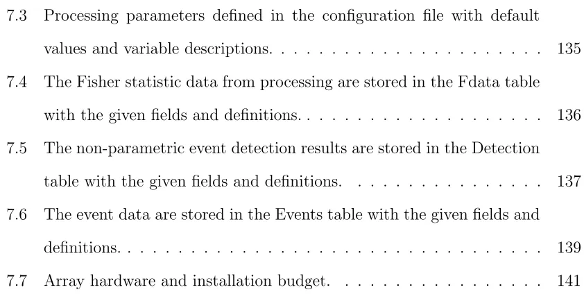
values and variable descriptions. . . 135 7.4 The Fisher statistic data from processing are stored in the Fdata table
with the given fields and definitions. . . 136 7.5 The non-parametric event detection results are stored in the Detection
table with the given fields and definitions. . . 137 7.6 The event data are stored in the Events table with the given fields and
definitions. . . 139 7.7 Array hardware and installation budget. . . 141
1.1 Interaction of factors that can lead to an avalanche. . . 2 1.2 The Snow Micro Penetrometer being used to evaluate snowpack layering. 5
2.1 The number of avalanches that hit Highway 21 in relation to the num-ber of days Highway 21 is closed. . . 10 2.2 Location of current avalanche forecasting operations by ITD for
High-way 21 and HighHigh-way 12. . . 11 2.3 A planar snow slab on an inclineθ. From Conway and Wilbour (1999). 12 2.4 The relationship between shear stress σf and snow density ρs can be
represented by a power law relationship. From Jamieson (1995). . . . 14 2.5 Flow chart for real time application of SNOSS. Three independent
processes occur to obtain weather data, run SNOSS, and view the results on a webpage. . . 18 2.6 Real time SNOSS webpage output, updated when a new weather
mea-surement is acquired. The top panel shows the hourly precipitation measurement, the middle panel is the time to failure, and the bottom panel is the stability index. . . 21 2.7 The new results figure was used starting for the 2012/2013 winter,
which includes hourly precipitation, temperature, minimum SI and the estimated depth, and the SI for all layers. . . 22
weather and SNOSS results. Hovering over a data point brings up a tool tip and shows the time and value of the point. . . 23 2.9 SNOSS model output of the stability index for a large storm that
produced 57 avalanches (more avalanche cycle information in Chapter 6). The black lines indicate two avalanche events that were identified through infrasound. . . 24
3.1 Avalanche paths along Little Cottonwood Canyon that have the ability to affect the road. . . 30 3.2 Flow chart for balanced random forests. Definitions: CT -
Classifica-tion tree; OOB - Out-of-Bag . . . 36 3.3 (a) UAA, (b) the true positive rate, or sensitivity, and (c) the true
negative rate, or specificity. . . 39 3.4 The top ten most important variables for the different predictor
vari-able tests. The bar represents one standard deviation about the mean. (a) All variables, (b) important variables, (c) meteorological variables, and (d) SNOSS variables. . . 40 3.5 The distribution of the probability of an avalanche occurring (a) given
the current conditions that produced a natural avalanche and (b) con-ditions when no avalanches occurred. . . 41
4.1 Typical crystals found at Grand Mesa for a) precipitation particles, b) rounded grains, and c) large facets. Scale is 1 mm between tick marks. 51
aries can differ between pit measurements and the SMP signal. Some pit measurements are similar to the manual delineation, however some layer boundaries are up to 20 mm off. . . 55 4.3 Flow chart of the random forest process. Definitions: CT -
classifi-cation tree; OOB - out-of-bag; B - bootstrap sample. See text for in-depth explanations. . . 59 4.4 Monte Carlo results using the mean, standard deviation, and CV(F)
predictors for random forests (RF) and a single classification tree (CT). The results between RF and CT are statistically different with lower error rates for RF at all sites. . . 63 4.5 Variable importance for simultaneously classifying three grain types
with mean, standard deviation, and CV(F) predictor variables. The bars show two standard deviations about the mean over the Monte Carlo simulations. Negative values occur when there is a decrease in the error rate after adding noise to the mth variable. Organized by highest to lowest Global importance. . . 65 4.6 Variable importance for binary classification of three grain types, using
the mean, standard deviation, and CV(F) predictor variables. The bars show two standard deviations about the mean over the Monte Carlo simulations. Organized by highest to lowest mean Global importance. 68
5.1 Dry avalanche flow, showing the three layers and possible sources of both infrasound and seismic signals. FromKogelnig et al. (2011). . . 75
paths. The avalanche path colors indicate return frequency of avalanches that reach Highway 21 with frequent avalanches (red,≥2 per year), oc-casional avalanches (yellow, 1-2 per year), and infrequent avalanches (green,≤1 per year). . . 78 5.3 a) The incidence angle i is the angle from vertical at which the wave
front reaches the array. b) The bearing from North to the source is the back azimuthθ. Triangles are example sensor locations. . . 81 5.4 Slowness vectors broken down to it’s components sx,sy, and sz. shor
is the slowness vector in the x−y plane. . . 82 5.5 A window of Fisher statistic values creates the background model PDF.
A new value of the Fisher statistic is then compared to the PDF with noise expected to fall within the distribution and an event to fall to the right of the distribution. Red dashed lines show how the current value, either noise or an event, will fall on the PDF. . . 88 5.6 Small wet avalanche that occurred during the 2-day avalanche cycle.
(a) The Fisher statistic was calculated over nine, 2 Hz frequency bands with most correlated energy in the 4-12 Hz bandwidth. (b) Amplitude signal of the avalanche. The start and end times of the avalanche are shown in red. Note that the avalanche has a small amplitude signal followed by uncorrelated wind signal. This signal is an avalanche as the back azimuth and vapp correspond to a known avalanche path. . . 91 5.7 Cycle background compared to the six events. . . 92
the residual. High significance level and small window sizes produce the most error in the detection with almost perfect detection in dark blue. The most accurate detection occurs with an alpha value around 10−10 and a window size greater than 600 seconds. . . . 94 5.9 Detection of the small wet avalanche. (a) Fisher statistic values. (b)
Probability of the current observation, low values indicate a new obser-vation and high values indicate a value that has been observed before. (c) Product of the probabilities in black with the automatic detection in green. The red lines indicate the actual start and end time of the avalanche. . . 95 5.10 The mean and standard deviation of the l2-norm for all the events. . 96 5.11 Median values of the l2-norm for all six event types identified. . . . . 97 5.12 Avalanche neural network results for classifying an avalanche as an
avalanche and an airplane as not an avalanche. FromHavens et al.(In Prep). . . 98 5.13 Vehicle neural network results for classifying a vehicle as a vehicle and
an avalanche as not a vehicle. FromHavens et al. (In Prep). . . 98
tral Idaho. A significant number of the major avalanche paths had evidence of extremely large dry avalanches, which occurred during the 19 January 2012 cycle. A total of 57 avalanches were reported in the area, with 37 avalanches that covered the highway with 1.5 to 8 me-ters of snow. b) Three-dimensional rendering obtained from a 2 meter aerial LiDar survey, overlain with 0.5 meter ortho photo. The maxi-mum extent of 96.92 is outlined in red with the path profile in blue. The infrasound array was located at the red marker. c) Head avalanche forecaster standing in the middle of the debris pile a day after the 96.92 avalanche event. The debris was approximately 8 meters high on the highway and continued to flow into the creek below. The array location is on the small ridge directly behind the forecaster. . . 107 6.2 (a) Avalanche signal with the three phases marked. The highest
am-plitude recorded at the array of 1.5 Pa occurred when the avalanche reached the highway. Inlay shows the whumpf signal with a two order of magnitude difference in amplitude. (b) Power spectrum of avalanche with the most power in the 1-10 Hz bandwidth. Higher frequencies ap-pear after avalanche reaches the highway. . . 109
period, the precursory signal, and the avalanche are compared. The Fisher statistic threshold was the 0.99 quantile of the signal-free period. The median value of the signals over the threshold was the signal-to-noise ratio (SNR), with the precursory and avalanche signal well above the Fisher statistic threshold value. . . 112 6.4 (a) F-statistic evaluated at each point along the path profile in the
1-10 Hz bandwidth. The three avalanche phases are shown with the highway location highlighted in purple. (b) Velocity of avalanche was slow to start, but reaches a maximum of 35.9±7.6ms−1 just before reaching the highway. (c) The 96.92 path profile in dashed red with a histogram of the maximum F-statistic locations through time. The solid red shows the maximum extent of the 96.92 avalanche path with the snowpack failure and avalanche motion originating around 300-320 meters. . . 115
7.1 The number of avalanches that hit Highway 21 in relation to the num-ber of days Highway 21 is closed. . . 121 7.2 Flow chart representing the processing steps for the real time
imple-mentation. . . 123 7.3 Quanterra Q330S data logger from Kinemetrics. . . 124 7.4 The fit-PC2i from fitPC. . . 126
batteries, ∼150Ah. (b) Charge controller to manage charging of bat-teries from solar panels. (c) FitPC. (d) Power box with two 12V and two 5V outputs. (e) Iridium satellite modem. (f) Q330S. . . 128 7.6 GUI on-site that controls the Q330S communication and processing.
The left panel buttons control starting and stopping of netmon, qmaserv, and datalog (through netmon). The left panel update button will up-date the status for netmon, datalog, and qmaserv from the log files. The right panel controls the processing flow and the update button will update the status of the processing from the log file. . . 130 7.7 Flow chart for the the on-site data retrieval and processing. . . 131
A.1 Compaction of polar snow in Antarctica where the pressure from the overburden changes the density of the snow and ice. FromMaeno and
Ebinumae (1983). . . 163
B.1 From Surinach et al. (2000). Station H is in the runout zone and station T is mid-path. E1, E2, and E3 correspond to different arrival times of different seismic signals. . . 167
CHAPTER 1:
INTRODUCTION
Avalanches occur when the snowpack fails, releasing a portion of the snowpack that begins to rapidly move downslope. The failure can occur when a cohensionless surface layer releases or as a cohesive block of snow that produces a loose snow avalanche or slab avalanche, respectively. Slab avalanches are a cohesive block of snow that fractures at a weak layer and can propagate for large distances before moving downslope. The failure layer for slab avalanches occurs on a buried layer due to new snow instabilities or on a persistent weak layer.
In the United States, most avalanches occur in remote mountainous regions and do not have a direct impact on infrastructure. When avalanches do pose a threat to infrastructure, they can prove hazardous to residential construction, highways, rail-roads, mountain travelers, utilities, commercial/industrial use, ski areas, and recre-ational users (Mears, 1992). In Ketchum, Idaho, homes are encroaching on avalanche terrain and the number of avalanche incidents are on the rise (Kellam, 2012). In-terstate 90 in Washington was closed for 89 hours in January-February 2008, which produced an estimated economic loss of just under $28 million dollars (Ivanov et al., 2008).
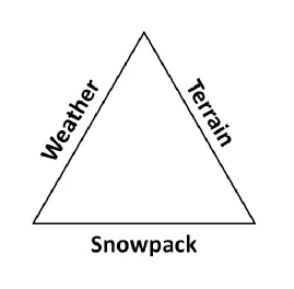
factors (Figure 1.1), but also the complexities within each factor. For an avalanche to occur, the snowpack must be unstable, which can be caused from too much load on an internal weak layer. Understanding the snowpack at a single point on a slope can be helpful but the snowpack properties can change drastically over short length scales due to weather and terrain factors.
The weather plays an important role in applying an increased load to the snowpack either from new precipitation or wind deposited snow. When a new layer forms and becomes part of the snowpack, there is possibility that the layer may become the instability within the snowpack. Even clear weather can adversely affect the snowpack through the formation of near surface facets or surface hoar that occur due to the energy balance at the surface.
Figure 1.1: Interaction of factors that can lead to an avalanche.
avalanche because the terrain is not capable of such an event. Therefore, a slope (typically 38o) is required to begin moving the snowpack downhill after release. There are many terrain factors that can lead to stability or instability within the snowpack. For example, a convexity in the slope will put the snowpack layers under greater stress, making it easier to trigger an avalanche.
These three factors - snowpack, weather, and terrain - must work together to create an unstable slope. The factors can produce a highly spatially variable snowpack that is difficult to evaluate. My work focuses on how to use snowpack properties at a point, either measured or modeled, and how to relate those properties to avalanche occurrences.
1.1
Snow Slope Stability at a Point
The snowpack is a collection of different layers that form from new or blowing snow. The different layers lead to stability problems when two snowpack layers have large differences in grain size, grain type, and hardness. The snowpack can be esti-mated with models that use weather data like precipitation and air temperature to model the snowpack (e.g., SNOWPACK Bartelt and Lehning, 2002; Lehning et al., 2002a,b). The models can provide insight as to how the snowpack is evolving through time when manual snowpack observations are not feasible.
avalanches are expected to occur within a region. Modeling the snowpack over a large landscape can be very problematic as both weather and terrain factors must be taken into account, which leads to a complex spatially distributed snowpack.
1.2
Measuring Snowpack Properties
The snowpack at a point must be evaluated to determine the snowpack properties, either for stability assessment or model validation. The current method of measur-ing snowpack properties is through a manual snow pit that is highly dependent on observer skill. Manual snow pits can contain errors in the location of layer bound-aries, grain size, and grain type (Pielmeier and Schneebeli, 2003). Therefore, a robust method to quickly characterize snowpack properties is needed.
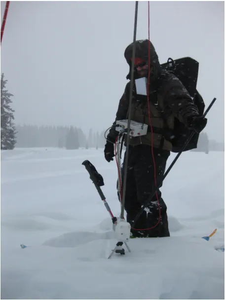
The Snow Micro Penetrometer (SMP, Schneebeli and Johnson, 1998) is an in-strument that takes mechanical snowpack profiles at speeds much greater than a traditional snowpit. The signal from the SMP (Figure 1.2) can be used to estimate snowpack properties like grain type, grain size, hardness, and strength. Certain mi-crostructural properties estimated through the SMP inversion procedure agree well with previous studies of measured parameters and make physical sense, while others do not (Marshall and Johnson, 2009). Using tools like the SMP can provide a method of characterizing the snowpack that is faster and can provide more spatial information than a traditional snowpit for both stability and model verification.
micromechanical properties from the SMP can then be used to classify the snowpack into precipitation particles, rounded grains, and faceted grains.
Figure 1.2: The Snow Micro Penetrometer being used to evaluate snowpack layering.
1.3
Understanding Where and When Avalanches
Occur
when an avalanche occurred until a much later time. We are left to hypothesize when the avalanche occurred based solely on our understanding of the current snowpack and weather conditions.
Avalanches emit low frequency noise (1-10 HzBedard Jr. et al., 1988) that is below the level of human hearing. Using instruments that are sensitive to infrasound (1-20 Hz band), we aim to detect avalanches that occur within a small mountainous region. This information will be valuable for highway department avalanche forecasters as large avalanches can be detected to determine if a road has been affected. Information on smaller avalanches that do not affect a road can be useful as an indicator of the instability being released from the snowpack.
To properly tune an avalanche forecasting model, the avalanche times must be known with some accuracy. Infrasound provides a method to accurately determine the avalanche time for a small region. The time can be fed back to the forecasting model, like SNOSS, to ensure that modeled stability is low when the avalanches are occurring. Chritin et al.(1996) used infrasound arrays to determine avalanche times, which updated a nearest neighbor forecasting model. Infrasound combined with a forecasting model tuned to actual avalanche times can provide avalanche forecasters with the ability to not only forecast when an avalanche may occur, but detect when and where avalanches are occurring.
1.4
Dissertation Organization
This dissertation is organized to address point scale measurements of the snow-pack. Appendix A reviews the current knowledge of snow densification. Chapter 2 and 3 evaluate the SNOw Slope Stability (SNOSS) model at a point. The goal is to use SNOSS as a tool to help avalanche forecasters evaluate avalanche hazard. By applying SNOSS to a large dataset of avalanche and weather observations, factors that produce natural avalanches can be explored.
Chapter 4 shows how the SMP can be used as a tool to classify grain types in support of remote sensing validation campaigns. The differences in grain types within the snowpack affect remote sensing measurements of snow water equivalent (SWE) and are an important factor to include in SWE retrieval algorithms. A relatively new classification technique is applied to a large database of SMP measurements in different types of snow in Switzerland and Colorado.
Chapter 5 provides the background information on avalanche infrasound gener-ation, current infrasound research, and array processing techniques. Chapter 5 and Chapter 6 use infrasound emitted by avalanches to detect and track where and when an avalanche occurs. Four winters of avalanche activity have been recorded along Highway 21 in Central Idaho. Automatic avalanche detection is explored using array processing techniques combined with non-parametric background modeling to deter-mine when infrasound signal is present (Chapter 5). In Chapter 6, I calculate the avalanche velocity of a fast moving avalanche at a high spatial and temporal resolu-tion.
array to detect when and where an avalanche occurs in real time. When an avalanche is detected by the on-site computer processing the data in near real time, the system will send out a message to alert the avalanche forecasters of the event.
Appendix B provides a literature review of seismic detection of avalanches. De-tection with infrasound will borrow heavily from the seismic community and under-standing the latest in seismic detection is critical.
1.5
Published Papers
Two chapters in this dissertation have been published in peer reviewed journals. The first paper was titled “Automatic Grain Type Classification of Snow Micro Pen-etrometer Signals with Random Forests” and was published in IEEE Transactions
on Geoscience and Remote Sensing (Havens et al., 2013). This paper is shown in
Chapter 4.
The second paper was titled “Calculating the Velocity of a Fast Moving Snow Avalanche Using an Infrasound Array” and was published in Geophysical Research
CHAPTER 2:
REAL TIME SNOW SLOPE STABILITY
MODELING
2.1
Research Project Statement
Avalanches routinely occur on Highways 21 and 12 each winter, posing a safety threat to maintenance workers and the traveling public. Currently, avalanche fore-casters based in Lowman, ID forecast for Highway 21 between Grandjean and Stanley, ID and Highway 12 near Lolo Pass, ID. An avalanche forecasting model would pro-vide avalanche forecasters with an additional tool when evaluating the possibility of avalanche activity. The work aims to enhance avalanche forecast accuracy, especially during darkness and for highway areas (like Highway 12) a long distance from the forecast office. During times of avalanche activity, Highway 21 routinely closes until the end of an avalanche cycle and reopens after the clean up effort. The goal of the ITD avalanche forecasters is to maintain the public safety while trying to keep Highway 21 open (Figure 2.1).
2.2
Study Site
Figure 2.1: The number of avalanches that hit Highway 21 in relation to the number of days Highway 21 is closed.
average), extremely cold temperatures between storms (-30 to -15 C), and rain on snow events throughout the winter. ITD has a limited explosive avalanche mitigation program due to the complex terrain in the start zones and the highway location. Avalanche activity is mostly direct action avalanches due to storm snow or rain on snow, with at least one major wet slide cycle during the spring. Both lanes of Highway 21 are frequently covered during avalanche cycles and the road is often closed for several days at a time.
meters above sea level) and frequently encounters rain on snow events.
Boise
Highway 21 Highway 12
Figure 2.2: Location of current avalanche forecasting operations by ITD for Highway 21 and Highway 12.
2.3
SNOw Slope Stability Model
The SNOw Slope Stability (SNOSS) model developed by Conway and Wilbour
2.3.1
Overburden Shear Stress
The stress applied by the snow slab in the down slope direction is the overburden shear stress σxz(t). The shear stress is a function of the amount of overburden snow above a given layer and a function of time as more snow layers are added from precipitation events. The shear stress at the base of the layer is dependent on the weight of water above the layer and is formulated as:
σxz(t) = g
Z
˙
Pwcosθsinθdt (2.1)
where g is the gravitational constant, P˙w is the accumulation rate, and θ is the slope angle (Figure 2.3). The accumulation rate is measured at precipitation gauges, typically at hour increments.
2.3.2
Basal Shear Strength
The strength of a weak layer is highly dependent on snow microstructure and crystal type. A first order approximation of a weak layers shear strength is to relate the shear strength to the snow density. Jamieson (1995) performed numerous field measurements of shear strength of persistent weak layers and their associated density. Jamieson’s results show a power law relationship between shear fracture strength and density:
σf =A1
ρs
ρi
2
(2.2)
where ρs and ρi are the density of snow and ice respectively. The parameter A1 is estimated from the measurements and varies from 1.8×10⁴Pa for faceted grains to 2.2×10⁴Pa for decomposing new snow with the best fit to all the measurements of
A1 = 1.95×10⁴Pa. However, Figure 2.4 shows a large range in strength for any given density, which can be attributed to different grain types or microstructural differences.
2.3.3
Snow Densification
The viscosity relates the stress to the strain rate through the following constitutive equation:
˙
= σ
ηz
(2.3)
where ηz is the compactive viscosity of the snow layer. The overburden stressσzz(t) contributes to the stress applied to the snow layer and for an inclined snowpack
σzz(t) = g
R ˙
Figure 2.4: The relationship between shear stress σf and snow density ρs can be represented by a power law relationship. From Jamieson (1995).
metamorphic component has a value of 75 Pa during a storm, where we expect equi-librium metamorphism to dominate especially near the surface whenσzz(t)≈0 (
Mar-shall et al., 1999). A snow layer with thickness h and density ρ compacted over a
time t will have a thickness of h −dh and density of ρ+dρ. Therefore, the new constitutive equation is:
˙
(t) = − 1
h(t)
dh
dt =
1
ρ(t)
dρ
dt =
1
ηz(t)
[σm(t) +σzz(t)] (2.4)
Kojima (1967) performed numerous field measurements over multiple seasons to
the affect of layer temperature on snow densification:
ηz(t) =B1eB2(ρz(t)/ρi)eE/(RTz) (2.5)
where B1 = 6.5×10⁻⁷Pa s, B2 = 19.3, the activation energy E = 67.3 kJ−1mol−1, the gas constantR = 0.0083 kJ mol−1K−1, and the layer temperature T
z in Kelvin.
2.3.4
New Snow Density
Equation 2.4 requires an estimate of the density of any new snow layer. New snow density is not measured at the hourly time scale and must be estimated with a representative model (reference unknown).
ρ0 = 134.2e(19.95Ta)/(273+Ta) (2.6)
where Ta is the air temperature in Celsius. This approximation has a significant amount of uncertainty since it does not take other weather parameters into account, like wind.
2.3.5
Stability Index
The ratio of the shear strength σf z to the overburden shear stress σxz is the stability index (Fohn, 1987) and is calculated for each layer at depth z:
Σz(t) =
σf z(t)
σxz(t)
As the value approaches 1, the probability of an avalanche theoretically increases. However, past studies have shown that avalanches typically occur at a higher stability index value (e.g., above 1.4), which varies between sites (Conway and Wilbour, 1999;
Lehning et al., 2004; Schweizer et al., 2006). This is possibly due to a difference
in model forcings and snowpack properties between available weather stations and starting zones.
2.3.6
Time to Failure
The time to failure is the expected length in hours until the critical stability index is reached. The time to failure assumes the current conditions stay the same and the slope of the stability index at the current time does not change.
tf(t) =
Σz(t)−Σc
dΣz/dt
(2.8)
where dΣz/dt is the slope of the stability value for the layer at the current time and Σc is the critical stability index value, typically set to 1 when failure is expected as the overburden shear stress reaches the layers shear strength.
2.3.7
Model Calibration
parameters were determined by changingB1 andB2 until the root mean square error (RMSE) was minimized. The results producedB1 = 2.69×10⁻⁸Pa s andB2 = 30.27, which are significantly different than the values found for the maritime climate of Washington in Conway and Wilbour (1999).
The second step of calibration is avalanche times, which are used to calibrate the basal shear strength (Equation 2.2) and provide insight into the significant values for the stability index and time to failure. However, determining when an avalanche has occurred can prove problematic along Highway 21 as the road can be closed for multiple days at a time, making visual confirmation of an avalanche occurrence not possible for hours to days after the avalanche event. What is required for proper calibration is sub hourly resolution of when the avalanche events occurred. To perform the calibration, we have deployed infrasound arrays to detect when and where an avalanche has occurred (Chapter 5) but the catalog of avalanche events is still under development.
2.4
Real Time Application
Download data from Mesowest New weather data? Wait for next run
Add station data to database No Yes Weather Database Load weather data SNOSS Results Database New precipitation?
Create new layer Yes Snowpack densification No Update strength Calculate SI
Add results to database Wait for next run Weather SNOSS Web Server
Figure 2.5: Flow chart for real time application of SNOSS. Three independent pro-cesses occur to obtain weather data, run SNOSS, and view the results on a webpage.
2.4.1
Weather Data
Mesowest collects, processes, archives, integrates, and disseminates weather data collected from over 43,000 automated weather stations (Horel et al., 2002). Mesowest has two methods for obtaining real time data: first through a file located on their FTP server, which is updated four times an hour. The second method is in beta testing but uses an Application Programming Interface (API) to provide data through a web service. For this project, the weather data is downloaded from the FTP server.
through the file for the desired weather stations. If the weather station is found, the data is added to a MySQL database (Figure 2.5). Typically, new weather data is available approximately 20 to 30 minutes after the measurement.
2.4.2
SNOSS
The real time application of SNOSS can be run for any weather station with a minimum of hourly temperature and precipitation measurements. SNOSS is run four times an hour to ensure the most up to date results. When only one new measurement exists for a station, the processing time is less than one second and 2,100 hourly measurements can be processed in approximately 10 seconds.
The flow chart in Figure 2.5 outlines the processing flow for SNOSS. For each weather station, the previous SNOSS results are loaded along with new weather data obtained since the last model run. If there is precipitation for that time step, a new layer is created with an initial density based on the air temperature. The algorithm proceeds with snow densification given the overburden and viscosity for each layer (Equations 2.4 and 2.5) and the new layer densities are calculated. Given the new layer densities, the shear strength is updated. Finally, the stability index (Equation 2.7) is calculated for each layer with the new strength and overburden.
2.4.3
Displaying Results on a Webpage
Over the life of the project, the results have been presented on a webpage in three different iterations, which are listed below.
1) First MATLAB Figures
The first results (Figure 2.6) tracked the basal layer from the beginning of the current storm. After 12 hours of no new precipitation, SNOSS began tracking the basal layer of the next storm, when precipitation resumes. However, tracking only the basal layer posed problems if the possible failure layer was not the basal layer due to initial density changes within the new snow.
Figure 2.6 shows the typical results displayed for the winter of 2011/2012 and how to interpret the figure. The figures were created in MATLAB and uploaded to the web server where the avalanche forecasters could look at the image. The figure worked well initially, but was not as informative or straight forward to interpret. If the basal layer was not the failure layer, the figure would not be able to effectively communicate the other potential weak layer.
2) Second MATLAB Figures
Wx Sta'on code Time figure was created
Current 'me step values
Time2Fail = 1
StabilityIndex = 1
Pr
eci
p [
in/hr
]
Tim
e t
o
F
ai
lu
re
[h
r]
St
ab
ili
ty
In
de
x
Figure 2.6: Real time SNOSS webpage output, updated when a new weather mea-surement is acquired. The top panel shows the hourly precipitation meamea-surement, the middle panel is the time to failure, and the bottom panel is the stability index.
Figure 2.7: The new results figure was used starting for the 2012/2013 winter, which includes hourly precipitation, temperature, minimum SI and the estimated depth, and the SI for all layers.
3) Web-Based Plotting Charts
Figures created in MATLAB are difficult to interact with and do not provide an easy way to look up past data without storing all of the past images. Many options exist for web-based plotting; I chose to use jqPlot (www.jqPlot.com) which is a javascript/jQuery based plotting library. jqPlot was chosen due to the elegant look and its ability to interact with the data.
that point. Web-based plotting allows the ITD avalanche forecasters an easy and interactive method to look at weather and SNOSS results.
Figure 2.8: Example of the new webpage design with new charts to display the weather and SNOSS results. Hovering over a data point brings up a tool tip and shows the time and value of the point.
2.5
Conclusion
The simple 1-D snow densification model SNOSS forecasts for direct action avalanches using the stability index. I have adapted SNOSS to run in real time and provides the ITD avalanche forecasters an additional tool for their avalanche forecasting op-eration. SNOSS runs by using weather data obtained from Mesowest and models how new snowfall creates instability within the new snow. The SNOSS results are displayed on a webpage using an elegant and interactive plotting library. The charts allow the ITD avalanche forecasters to look quickly at weather and model results for any desired date and station.
in-estimated layer height [m]
Stability Index − BNRI1
0 0.1 0.2 0.3 0.4 0.5 0.6 0.7
1 1.5 2 2.5 3 3.5 4 4.5 5
Wed 00:00 Thu 00:00 Fri 00:00 Sat 00:00 Sun 00:00 Mon 00:00
0 1 2 3 4 5
Minimum SI value
Avalanche Times
Figure 2.9: SNOSS model output of the stability index for a large storm that produced 57 avalanches (more avalanche cycle information in Chapter 6). The black lines indicate two avalanche events that were identified through infrasound.
CHAPTER 3:
AVALANCHE CLASSIFICATION WITH
BALANCED RANDOM FORESTS AND
SNOWPACK MODELING
3.1
Abstract
3.2
Introduction
Avalanche forecasting models ingest weather and snowpack data in order to deter-mine if the complex interaction of weather and snowpack data will lead to avalanche activity. Similar to an avalanche forecaster, the model attempts to use the available weather, snowpack, and avalanche information to determine if the current and future conditions will lead to avalanche activity. Avalanche forecasting models will not re-place the experience and knowledge of an avalanche forecaster any time soon, but will help communicate how the multitude of information relates to avalanche activity.
Previous studies have primarily used meteorological data to predict avalanche activity. The classification schemes use either manually collected weather data (Davis
et al., 1999; Floyer and McClung, 2003) or data from automatic weather stations
(Hendrikx et al., 2005; Cordy et al., 2009; Eckerstorfer and Christiansen, 2011). The
most popular method is to forecast avalanche days (i.e., whether or not an avalanche has occurred over a specified time window). These studies reported results that vary between a 70-85% correct classification rate for both natural and artificially released avalanches. The model results are simple to interpret but require a significant amount of past avalanche data to test the model. Classification performance improves with the quality of the meteorological data available.
data set for calibration to produce robust results.
Snowpack modeling can provide the required hourly snowpack property infor-mation that would be needed for avalanche forecasting models. Snowpack models typically use a minimum of hourly precipitation and temperature measurements, and from these measurements construct and evolve the snowpack through time. The phys-ically based SNOWPACK model (Bartelt and Lehning, 2002;Lehning et al., 2002a,b) has been used to create snow profiles during times of avalanche activity. Measured snowpack stability from pit and Ruchblock tests were compared with SNOWPACK outputs of snow strength to evaluate how well SNOWPACK can determine stability rating (Lehning et al., 2004; Schweizer et al., 2006; Schirmer et al., 2010). Schirmer
et al.(2010) found that SNOWPACK variables were better at detecting rather stable
conditions when compared with the regional avalanche hazard forecast. However, SNOWPACK has not been compared with a large database of avalanche activity to test the model results.
The French SAFRAN-Crocus-MEPRA (SCM) chain (Durand et al., 1999) is an operational avalanche forecasting model that uses meteorological data as input to the snowpack model Crocus. The results from Crocus are analyzed with an expert system of rules (MEPRA) to determine if natural or skier triggered avalanche activity is likely to occur.
estimate avalanche regional activity.
3.3
Study Site
The Utah Department of Transportation (UDOT) has an avalanche forecasting program for the Little Cottonwood Canyon road between Salt Lake City and Alta, Utah in the Wasatch Mountains (Figure 3.1). UDOT has an extensive explosive avalanche mitigation program employing multiple Avalaunchers and large artillery. Avalanche records affecting the road date back to 1974 and provide a large dataset of high quality avalanche observations alongside a long history of weather observations. A significant amount of the avalanches in the area are direct action avalanches due to storm snow and occur during or directly after a storm. However, the climate is intermountain and can produce depth hoar at the base of the snowpack during the early season. Here we focus on slide paths with multiple events per year to target direct action events. Avalanche records between years 2001 and 2010 were used along with data from two weather stations. Alta Guard (2682 meters) measures hourly precipitation, air temperature and snow accumulation on a storm board. Alta Baldy (3373 meters) measures air temperature, wind speed, and wind direction.
3.4
SNOw Slope Stability Model
The SNOw Slope Stability (SNOSS) model developed by Conway and Wilbour
LC1 LC2 LC3 ! !!!! ! !!!! !!!!! Gate B Gate A Gate F Gate D Gate C Gate E LITTLE PINE LISA FALLS OLD MILL ELBERT'S SLIDE 7 TURNS WHITE PINE ACORN TANNERS OAK RIDGE MORMON SLIDE GOAT COALPIT #4 MAYBIRD WILLOWS COTTONWOOD DRAW MONTE CRISTO GULLY MONTE CRISTO #10 SPRING FACE #10 SPRINGS GULLY TED'S HOUSE VALERIE'S HILTON MAIN SUPERIOR LITTLE SUPERIOR HELLGATE BACKBOWL HELLGATE BOWL EAST HELLGATE 64 CHUTE TOLEDO BOWL BLACKJACK CARDIFF
BOWL FLAGSTAFFSHOULDER FLAGSTAFF FACE EMMA #1 EMMA #2 EMMA #3 EMMA #4 CULPS GRIZZLY
#1 #2 #3 #4 WHITE PINE CHUTES LIMBER PINE JEDEDIAH LITTLE PINE EAST LODGE CORNER HIGH MODELS
Scale = 1:27,500 0 0.4 0.8 1.6
Miles
I
Figure 3.1: Avalanche paths along Little Cottonwood Canyon that have the ability to affect the road.
3.5
Methods
3.5.1
Natural Avalanche Days
for SNOSS. This ensures that the non-avalanche day does not contain any type of avalanche that would produce biased results.
Since we are looking at predicting natural avalanches that occur during storms, we want to have non-avalanche days that reflect times of significant storms. This will allow us to directly compare why certain storms produced avalanches and others did not. The criterion for a storm was more than 1.3 cm of water, less than 2 degrees C at the peak weather station, and less than 2 hours elapsed since the last precipitation measurement. These criteria produced 42 avalanche days and 358 non-avalanche days. The number of avalanches days already show that there are times of significant storms that still do not produce avalanches.
3.5.2
Meteorological and SNOSS Predictor Variables
For each avalanche day, meteorological and SNOSS predictor variables were cre-ated for the 12, 24, 48, and 72 hours prior to the end of each time window (Table 3.1). The minimum (Min), average (Avg), maximum (Max), and range (Range) values of the meteorological variables are calculated for each time window. Since total snow depth is not measured at Alta Guard, the hourly snow accumulation was determined when the snow board registered an increase in snow depth from the snow depth sen-sor placed on the snow board. The snow accumulation was then either summed or averaged for the time windows to create the total snow accumulation or average snow accumulation respectively. The snow drift parameter is the total water weight mea-sured at Alta Guard multiplied by the peak wind speed raised to the fourth power (i.e., Davis et al., 1999; Hendrikx et al., 2005).
Baldy were used to run SNOSS for the 12, 24, 48, and 72 hours windows. The minimum stability index and time to failure of the new snow was restricted to the last 12 hours of model output to ensure that the minimum value occurs in the avalanche day window. At the minimum stability index value (the most likely failure layer), the depth below the snow surface, layer settlement, and layer strength were used for the SNOSS predictor variables (Table 3.1).
A total of 108 predictor variables were created: 88 from meteorological factors and 20 from SNOSS model results (Table 3.1). A different subset of the predictor variables was used to determine the most important variables for predicting natural avalanches. The subsets included:
1. All the predictor variables
2. Significant meteorological and SNOSS variables (18 total)
3. Meteorological variables
4. SNOSS variables
The significant meteorological and SNOSS variables are the most significant variables from the all predictor variables tested.
3.5.3
Balanced Random Forests
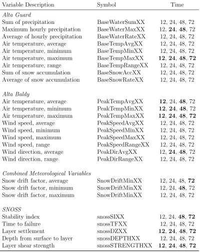
sam-Table 3.1: Meteorological and SNOSS predictor variables. XX denotes the time for each of the variables. Bold variables were used for the significant variable test.
Variable Description Symbol Time
Alta Guard
Sum of precipitation BaseWaterSumXX 12, 24, 48, 72
Maximum hourly precipitation BaseWaterMaxXX 12, 24, 48, 72 Average of hourly precipitation BaseWaterRateXX 12, 24, 48, 72 Air temperature, average BaseTempAvgXX 12, 24, 48, 72 Air temperature, minimum BaseTempMinXX 12, 24, 48, 72 Air temperature, maximum BaseTempMaxXX 12, 24, 48, 72
Air temperature, range BaseTempRangeXX 12, 24, 48, 72 Sum of snow accumulation BaseSnowAccXX 12, 24, 48, 72 Average of snow accumulation BaseSnowRateXX 12, 24, 48, 72
Alta Baldy
Air temperature, average PeakTempAvgXX 12, 24, 48, 72 Air temperature, minimum PeakTempMinXX 12,24, 48, 72 Air temperature, maximum PeakTempMaxXX 12, 24, 48, 72
Wind speed, average PeakSpeedAvgXX 12, 24, 48, 72
Wind speed, minimum PeakSpeedMinXX 12, 24, 48, 72
Wind speed, maximum PeakSpeedMaxXX 12, 24, 48, 72
Wind speed, range PeakSpeedRangeXX 12, 24, 48, 72
Wind direction, average PeakDirAvgXX 12, 24, 48, 72 Wind direction, range PeakDirRangeXX 12, 24, 48, 72
Combined Meteorological Variables
Snow drift factor, average SnowDriftMinXX 12, 24, 48, 72
Snow drift factor, minimum SnowDriftMinXX 12, 24, 48, 72 Snow drift factor, maximum SnowDriftMinXX 12, 24, 48, 72
SNOSS
Stability index snossSIXX 12, 24,48, 72
Time to failure snossTFXX 12, 24, 48, 72
Layer settlement snossDZXX 12, 24, 48, 72
pling reduces correlation between each classification tree in the ensemble leading to a stronger classifier.
Balanced Random Forests (BRF; Chen et al., 2004) are used when the dataset is imbalanced. This occurs when the class of interest (i.e., avalanche occurrence) is the minority class and contains significantly less values than the majority class. Classification of imbalanced datasets is biased towards the majority class where the highest accuracy can be obtained by correctly classifying only the majority class. However, the process ignores the minority class that we are interested in classifying and understanding.
A random forest randomly samples with replacement from all the dataset values to create a bootstrap sample (B) the same size as the original data. This can lead to problems with imbalanced classes because there is a high probability that the minority class will not be well represented in B. Therefore, Chen et al. (2004) proposed to randomly sample with replacement from each class separately. The minority class is randomly sampled with replacement to create a bootstrap sample that is the same size as the minority class. The same number of cases is randomly sampled with replacement from the majority class. This produces a bootstrap sample with an equal number of cases from each class. Class labels may appear multiple times or not at all in B. Cases that are not selected for B are considered out-of-bag (OOB) samples. On average,∼37% of the minority cases will be OOB and significantly more for the majority class.
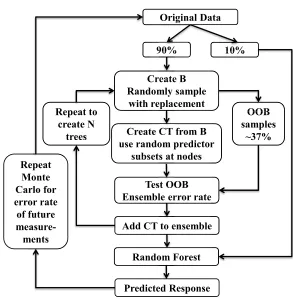
predictive power and reduces correlation between trees in the ensemble. The random selection of B was repeated for the desired number of trees, each time storing the OOB cases and the classification tree to create a BRF.
To make a prediction, the predictor variables are run through the BRF, producing a predicted class from each tree. In the majority of random forest studies, the class with the highest probability of classification is the predicted class. However, in this study, we are more interested in the probability of an avalanche given the current weather and snowpack model. The probability of an avalanche is determined from the number of trees predicting a class over the number of trees in the random for-est. A high probability indicates a high number of trees voted for the class and a low probability indicates a low number of trees voted for the class. Therefore, the probability of an avalanche will provide information to avalanche forecasters on the probability of an avalanche occurring given the current conditions.
The importance of a predictor variable can be determined from the change in error rate when noise is added to the mth variable. The mean change in error rate over the standard deviation of the change in error rate gives the variable importance. A variable with a high value indicates that the variable is important to distinguish between an avalanche and non-avalanche day.
3.5.4
Performance Evaluation
Original Data Randomly sample with replacement OOB samples Test OOB Ensemble error rate
Add CT to ensemble Create CT, use random
predictor subsets at nodes Repeat to create N trees Random Forest Predicted Response
Figure 3.2: Flow chart for balanced random forests. Definitions: CT - Classification tree; OOB - Out-of-Bag
cases are classified as avalanche day or non-avalanche day and a confusion matrix can be created.
Table 3.2: Confusion matrix. Observation
True Negative Total
Predicted True a b a+b
Negative c d c+d
Total a+c b+d N
To determine the accuracy, the unweighted average accuracy (UAA) metric will be used as this metric weights evenly the accuracy of predicting an avalanche day and the accuracy of predicting a non-avalanche day. The UAA is calculated
UAA = 0.5
a
a+c +
d
b+d
The creation of the BRF was repeated 100 times to estimate the uncertainty in the both the UAA and the probability of classification.
The true positive rate, or sensitivity, is a measure of how well the predictive model can identify the true class label. The sensitivity is defined as:
Sensitivity = a
a+c (3.2)
When the sensitivty approaches 1, the number of false negatives approaches 0, in-dicating that the majority of true classes are identified correctly. A low sensitivity means a high number of the true class were classified incorrectly (false negatives), indicating a poor predictive model.
The true negative rate, or specificity, is a measure of how well a predictive model can identify the false class label. The specificity is defined as:
Specificity = d
b+d (3.3)
3.6
Results
3.6.1
Overall Correct Classification
The average overall correct classification was low for all subsets of predictor vari-ables (Figure 3.3a). The significant varivari-ables had the lowest UAA with an overall correct classification only slightly better than a random guess (0.57). The sensitivity (Figure 3.3b) was low with an average value of 0.4, which indicates that the avalanche days were not being correctly identified (a high false negative). The specificity (Fig-ure 3.3c) was within reason at 0.75, which indicates that the non-avalanche days were being correctly identified, and a limited number were classified as an avalanche day.
The second lowest scoring test was using only SNOSS predictor variables with an average UAA of 0.62 (Figure 3.3a). The sensitivity (Figure 3.3b) was higher with an average value of 0.55, which indicates that about half of the avalanche days were not being correctly identified (a high false negative). The specificity (Figure 3.3c) was the lowest of all tests at 0.71, which indicates that a significant number of non-avalanche days were being correctly identified, and a limited number were classified as an avalanche day.
better than the other tests. 0.5 0.55 0.6 0.65 0.7
All Sig Wx SNOSS
UAA (a) 0.3 0.35 0.4 0.45 0.5 0.55 0.6 0.65
All Sig Wx SNOSS
True Positive Rate (Sensitivity)
(b) 0.68 0.7 0.72 0.74 0.76 0.78 0.8 0.82
All Sig Wx SNOSS
True Negative Rate (Specificity)
(c)
Figure 3.3: (a) UAA, (b) the true positive rate, or sensitivity, and (c) the true negative rate, or specificity.
3.6.2
Variable Importance
The top ten most important variables for each test were evaluated using Fig-ure 3.4. There were four variables that were important for three out of the four tests: PeakTempMax48, SnowDriftMin48, snossSI48, and snossSTRENGTH12. Six variables were important for two out of the three tests: BaseTempMax48, BaseWater-Max24, snossDZ24, snossDZ72, snossSTRENGTH24, and snossSTRENGTH72. Six out of the top ten most frequent variables are attributed to SNOSS model outputs of settlement, strength, and the stability index. Out of the top 20 for all and important variables, 9 were from SNOSS and 11 were from meteorological variables.
−0.1 −0.05 0 0.05 0.1 0.15 0.2
snossDZ24 SnowDriftMin48 BaseTempMax48 snossDZ72 PeakTempMax48 snossSTRENGTH72 snossSTRENGTH12 snossSI48 snossSTRENGTH24 BaseTempMax72
Variable Importance All Variables (a) −0.1 0 0.1 0.2 0.3 0.4
snossSI48 PeakTempMax48 PeakTempAvg48 SnowDriftMin48 snossSTRENGTH12 snossSI72 PeakTempMin48 BaseWaterMax24 PeakTempMin24 PeakTempMax72
Variable Importance Important Variables (b) −0.2 −0.1 0 0.1 0.2
PeakTempMax48 BaseTempMax48 SnowDriftMin48 PeakDirAvg24 SnowDriftMin24 PeakDirAvg48 BaseWaterMax24 BaseWaterMax48 PeakTempMax12 PeakSpeedMin24
Variable Importance Meteorological Variables (c) −0.1 0 0.1 0.2 0.3
snossDZ24 snossSTRENGTH72 snossSI12 snossSTRENGTH12 snossDZ72 snossDZ48 snossSTRENGTH48 snossSTRENGTH24 snossSI48 snossDZ12
Variable Importance
SNOSS Variables
(d)
Figure 3.4: The top ten most important variables for the different predictor variable tests. The bar represents one standard deviation about the mean. (a) All variables, (b) important variables, (c) meteorological variables, and (d) SNOSS variables.
ten variables.
3.6.3
Probability of an Avalanche
Figure 3.5: The distribution of the probability of an avalanche occurring (a) given the current conditions that produced a natural avalanche and (b) conditions when no avalanches occurred.
around 0.41 with all other tests between 0.17 to 0.21. The non-avalanche day are those days that did not produce an avalanche and should have a lower probability of predicting an avalanche.
3.7
Discussion and Conclusion
A subset of the avalanche records at Alta, UT were used in order to determine when a natural soft slab avalanche will occur during a storm. Previous studies either randomly sampled non-avalanche days from the rest of the weather record (Hendrikx
the data from the previous seasons (Cordy et al., 2009). These studies attempted to predict all avalanche activity, both natural and artificial. Since we are attempting to predict natural avalanches due to new snow loading, the non-avalanche and avalanche days consisted of large storms with more than 1.3 cm of water. This creates a difficult classification problem to try and predict whether or not an avalanche will occur in a storm.
Balanced random forests (BRF;Chen et al., 2004) is a method of implementing the random forest procedure outlined byBreiman (2001). BRF account for an unbalanced dataset and randomly sample the inputs based on the smallest class size, reducing classification bias. BRF benefit when variables are correlated as the random sampling at each stage reduces the affect of correlation between variables (Breiman, 1996, 2001). This allows for a large amount of predictor variables from 12, 24, 48, and 72 hours prior to the avalanche day.
Other studies that use classification trees (Davis et al., 1999; Hendrikx et al., 2005) or nearest neighbor techniques (Purves et al., 2003; Cordy et al., 2009) have only used meteorological variables. This is the first study to try and relate the snow pack model SNOSS, along with meteorological variables, to avalanche activity. The average overall correct classification for predicting natural soft slab avalanche activity during a storm was between 57% to 67%. The sensitivity (Figure 3.3b) shows that only about 55% of the avalanche days were being correctly identified. This indicates that there may be other variables that we could not account for, like a persistent weak layer. If persistent weak layers were present, SNOSS would not be able to predict instability and the model would have to rely on the meteorological variables.
Peak-TempMax48, SnowDriftMin48, snossSI48, snossSTRENGTH12, BasePeak-TempMax48, BaseWaterMax24, snossDZ24, snossDZ72, snossSTRENGTH24, and snossSTRENGTH72. The snow drift parameter has shown up before in a study performed at Alta, UT
(Davis et al., 1999) and in maritime climates (Hendrikx et al., 2005). The other
important variables are based on the air temperature and the maximum hourly pre-cipitation rate or intensity (BaseWaterMax24). All important SNOSS variables have a quantitative meaning to the snowpack. The settlement of the failure layer calcu-lated from SNOSS appears to be the most important SNOSS variable in separating avalanche from non-avalanche day with the snow layer strength also an important predictor.
Instead of a “yes” or “no” vote from the BRF, the number of trees within the BRF voting for an avalanche is the probability of an avalanche given the current conditions. The distributions between the two days (Figure 3.5) are quite different as the probability distribution is skewed towards higher probabilities when a natural avalanche has occurred. This shows that the BRF predicts a higher probability of an avalanche when a natural avalanche occurred. The error rates (Figure 3.3a) reflect a cutoff value of 50% of the trees voting for a particular class. It may be that the cutoff value is actually lower since most avalanches are centered around the 52% to 55% range. Error rates may improve by optimizing the cutoff value.
Acknowledgements
CHAPTER 4:
SNOW MICRO PENETROMETER SIGNAL
CLASSIFICATION WITH RANDOM FORESTS
Summary
The spatial variability of snowpack properties can be fairly difficult to measure given the current method of snow pits. Snow pits are highly subjective to observer skill and can take a significant amount of time to complete. Digging multiple snow pits for spatial variability studies is time intensive and may not be able to accurately capture the true variability. The Snow Micro Penetrometer (SMP) is a tool that can take full mechanical profiles of the snowpack in only a couple of minutes. With the SMP, it is possible to cover large distances while getting useful mechanical snowpack profiles.
This work is the first step in the direction of using the SMP to automatically classify grain types. While on a remote sensing and validation campaign, the SMP can be used to classify the stratigraphy of an area at speeds much greater than the traditional snowpit. The results of this work show that we can classify the SMP signal into new snow, rounds, and facets using an ensemble of classification trees. Future work will include applying this technique to full SMP profiles, which will enable the user to quickly characterize a site.
The paper was published June 2013 in IEEE Transactions on Geoscience and
at Boise State University. This paper targets an audience in the snow remote sensing community to show the difficultly in representing a complex snowpack as a single grain type. We hope that our results will show that with different grain sizes, the grain sizes and shapes are significantly different and need to be accounted for in radiative transfer models or in snow water equivalent retrieval algorithms.
Automatic Grain Type Classification of
Snow Micro Penetrometer Signals with
Random Forests
Scott Havens∗, Hans-Peter Marshall∗, Christine Pielmeier,† and Kelly Elder‡
∗Center for Geophysical Investigation of the Shallow Subsurface, Boise State
University, Boise, Idaho, USA
†WSL Institute for Snow and Avalanche Research SLF, Davos, Switzerland ‡USDA Forest Service, Rocky Mountain Research Station, Fort Collins, CO, USA.
4.1
Abstract
random forest techniques to classify three snow grain types (new snow, rounds, and facets) from SMP measurements collected in Switzerland and Grand Mesa, Colorado. Random forests performed up to 8% better than single classification trees, with over-all misclassification errors between 17-40 percent. The coefficient of variation of the penetration force proved to be the most important variable, followed by variables that contain information about grain size like micro scale strength and the number of ruptures.
4.2
Introduction
The complicated structure of the seasonal snowpack is important for snow avalanches, snow hydrology, and microwave remote sensing. Snow microstructure controls snow strength and complicates retrieval of important hydrological quantities, such as snow water equivalent (SWE) for both passive and active radars (Rees, 2006; Baenninger
et al., 2008; Wojcik et al., 2008). Microstructural properties such as hardness, grain
size, and grain shape vary significantly between layers in the snowpack (e.g.,Pielmeier
and Schneebeli, 2003) and are important to characterize to properly describe the
sea-sonal snowpack (Shapiro et al., 1997).
Accurate and objective methods to determine snow stratigraphy are needed, as stratigraphy is a major influence on microwave emission models (Durand et al., 2008). Current algorithms assume a homogeneous one-layer snowpack, typically with grain size (and sometimes stickiness), as a tunable parameter that is chosen to minimize the error between in-situ ground data and estimates from microwave inversion algorithms
(Yueh et al., 2009; Rott et al., 2010). These techniques can produce errors in SWE