Patron: Her Majesty The Queen Rothamsted Research Harpenden, Herts, AL5 2JQ
Telephone: +44 (0)1582 763133 Web: http://www.rothamsted.ac.uk/
Rothamsted Research is a Company Limited by Guarantee Registered Office: as above. Registered in England No. 2393175.
Rothamsted Repository Download
A - Papers appearing in refereed journals
Dungan, J. L., Perry, J. N., Dale, M. R. T., Legendre, P., Citron-Pousty,
S., Fortin, M-J., Jakomulska, A., Miriti, M. and Rosenberg, M. S. 2002. A
balanced view of scale in spatial statistical analysis. Ecography. 25 (5),
pp. 626-640.
The publisher's version can be accessed at:
•
https://dx.doi.org/10.1034/j.1600-0587.2002.250510.x
The output can be accessed at:
https://repository.rothamsted.ac.uk/item/88wv4/a-balanced-view-of-scale-in-spatial-statistical-analysis.
© Please contact [email protected] for copyright queries.
ECOGRAPHY 25: 626 – 640, 2002
A balanced view of scale in spatial statistical analysis
J. L. Dungan, J. N. Perry, M. R. T. Dale, P. Legendre, S. Citron-Pousty, M.-J. Fortin, A. Jakomulska, M. Miriti and M. S. Rosenberg
Dungan, J. L., Perry, J. N., Dale, M. R. T., Legendre, P., Citron-Pousty, S. Fortin, M.-J., Jakomulska, A., Miriti, M. and Rosenberg, M. S. 2002. A balanced view of scale in spatial statistical analysis. – Ecography 25: 626 – 640.
Concepts of spatial scale, such as extent, grain, resolution, range, footprint, support and cartographic ratio are not interchangeable. Because of the potential confusion among the definitions of these terms, we suggest that authors avoid the term ‘‘scale’’ and instead refer to specific concepts. In particular, we are careful to discriminate between observation scales, scales of ecological phenomena and scales used in spatial statistical analysis. When scales of observation or analysis change, that is, when the unit size, shape, spacing or extent are altered, statistical results are expected to change. The kinds of results that may change include estimates of the population mean and variance, the strength and character of spatial autocorrelation and spatial anisotropy, patch and gap sizes and multivariate relationships. The first three of these results (precision of the mean, variance and spatial autocorrelation) can sometimes be estimated using geostatistical support-effect models. We present four case studies of organism abundance and cover illustrating some of these changes and how conclu-sions about ecological phenomena (process and structure) may be affected. We identify the influence of observational scale on statistical results as a subset of what geographers call the Modifiable Area Unit Problem (MAUP). The way to avoid the MAUP is by careful construction of sampling design and analysis. We recommend a set of considerations for sampling design to allow useful tests for specific scales of a phenomenon under study. We further recommend that ecological studies completely report all components of observation and analysis scales to increase the possibility of cross-study comparisons.
J.L.Dungan([email protected]6),MS242-2,NASA Ames Research Center, Moffett Field,CA94035-1000,USA. – J.N.Perry,Plant and In6ertebrate Ecology Di6.,Rothamsted Experimental Station,Harpenden,Herts,U.K.AL5 2JQ. –M.R.T. Dale,Dept of Biological Sciences,Uni6.of Alberta,Edmonton,AB,Canada T6G2E9. – P. Legendre, De´pt de Sciences Biol., Uni6. de Montre´al, C.P. 6128 succ. A, Montre´al,QC, Canada H3C3J7. – S.Citron-Pousty, Social Science Statlab, Yale Uni6.,140Prospect St.,P.O.Box208208,New Ha6en,CT06520-8208,USA. –M.-J. Fortin, Dept of Zoology, 25 Harbord St., Uni6. of Toronto, Toronto, ON, Canada M5S3G5. –A.Jakomulska,Remote Sensing of En6ironment Lab.,Fac.of Geography and Regional Studies,Uni6. of Warsaw, 26/28, PL-00-927 Warsaw, Poland. – M. Miriti, Dept of E6olution, Ecology and Organismal Biology, The Ohio State Uni6., 1735 Neil A6e., Columbus, OH 43210-1293, USA. – M. S. Rosenberg, Dept of Biology,Arizona State Uni6.,P.O.Box871501,Tempe,AZ85287-1501,USA.
Technological advances have improved researchers’ ca-pacity to observe phenomena that occur over very small (10−9 m) to very large (1014 m) extents. The increased use of new tools has created opportunities for collaboration among researchers from previously inde-pendent fields such as geology, cartography and
ecol-ogy. As the interests of these distinct fields continue to merge, the need for consistent, conforming terminology becomes increasingly important (Silbernagel 1997, Jenerette and Wu 1999, Csillag et al. 2000). ‘‘Scale’’ is one term that has gained great currency in ecology during the past decade (Wiens 1989, Levin 1992,
Accepted 6 February 2002
Ehleringer and Field 1993, Peterson and Parker 1998, Gardner et al. 2001), yet this term has multiple, some-times contradictory meanings.
One scale concept with a long tradition in geography is map scale, a cartographic ratio referring to the relationship between the distance or area represented
on a map to the corresponding real-world distance or area. In landscape ecology, scale has the disjunctive definition of ‘‘grain and extent’’ (Turner 1989). The term ‘‘resolution,’’ commonly used in remote sensing, is defined as the smallest object that can be reliably detected. A geostatistical term, ‘‘support,’’ has been used since the 1960s to refer to an n-dimensional vol-ume, including its geometrical shape, size and orienta-tion, within which average values of a variable may be computed (Olea 1990). Schneider (1994) devotes an entire text to concepts of spatial scaling in ecology. In fact, the word scale has a long and varied list of synonyms, including several more meanings in mathe-matics and statistics. Concepts such as cartographic ratio, grain, extent, resolution, support, range, variance and footprint have all been used as synonyms of scale in one context or another.
The purpose of this paper is to present a balanced view of scale terms by considering their specific mean-ings and their relationships to one another. We identify some of the most prevalent scale terms in ecology and propose that their definitions can be best understood within three categories or dimensions. We then review how changing scales within two of these categories (sampling and analysis) can make a substantial differ-ence to the inferdiffer-ences about the third category (phe-nomena). The relevance of changing scales is further discussed using four case studies. Finally, we recom-mend sampling design considerations that are specific to these dimensions of scale.
To provide a framework to discuss scale terms and to provide a means of reducing potential confusion over myriad definitions, we distinguish among three different categories to which spatial scale-related terms may be applied: 1) the phenomenon being studied, for example the spatial structure of vegetation and the processes that affect it; 2) the spatial units or sampling units used to acquire information about the phenomenon, for example quadrats on the ground or pixels in an image; and 3) the analysis of the data, used to summarize them or make inferences. The phenomenon, sampling and analysis categories can be thought of as three dimen-sions to which scale concepts pertain (Fig. 1). We will illustrate this idea with a simple example.
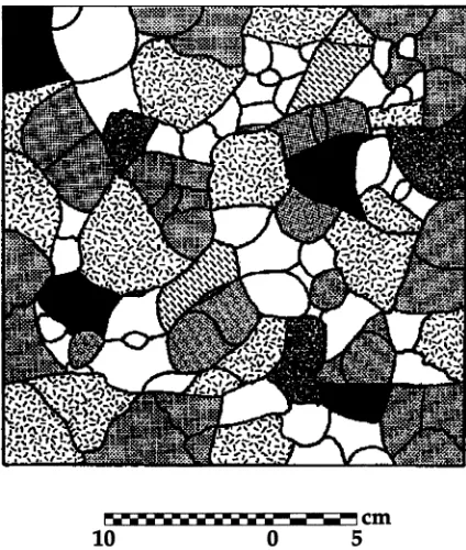
Consider a community of crustose lichens growing on a large smooth plane rock surface (Fig. 2). For the purposes of illustration, we will discuss a structurally simple system that is essentially two-dimensional. We will pretend that there is no environmental variability in this system, although in real saxicolous communities, differences in environmental conditions on a single rock face may determine where particular lichen species are found. Plant communities typically have many other complexities in their physical pattern arising from verti-cal structure and from variation in environmental (to-pographic, hydrologic, soil, climatic, etc.) variables. Fig. 1. Dimensions of scale concepts.
In our illustration, individual lichen bodies (thalli) are associated in monospecific clusters or patches, here called tiles. Boundaries between tiles separate thalli of the same or different species. There are also tiles of uncolonized rock. Together these tiles make up a mo-saic. If s is the number of lichen species, there are s+1 phases in this mosaic with the additional phase being the bare rock. At any point in time, there are at least two spatial characteristics of the structure or pattern of this mosaic (see the phenomenon axis in Fig. 1). One is the distribution of the tile sizes, which has a mean and variance. Of course, different species may have different tile size distributions. Another characteristic of the pat-tern is the spacing between tiles of the same phase. This spacing will vary with the commonness or rarity of a particular species and with whether colonies of the species tend to be clumped together in close proximity. These sizes and spacings, properties of the phenomenon of these lichens, are ecological subjects of interest.
Besides the physical structure of a system, the pro-cesses that act upon it have their own spatial character-istics. Again there are at least two for each process (see the phenomenon axis in Fig. 1). The first is the distance at which it can act, its range of action; the second is its potential or actual extent, the area that it does or can affect. For example, in the lichen community, the dis-persal of propagules (spores or soredia) may occur at a distance that is large relative to the size of the lichen thallus, but each propagule will, at least initially, affect only a very small area of the rock. Competition for space between thalli, if physical, may occur only at very short distances and may affect only small areas. If competition is mediated by the release of quantities of allelopathic chemicals, both the range of action and the spatial extent affected may be greater. Factors from outside the community itself, such as the disturbance of a boulder sliding across the rock and scraping the lichens off the surface, can affect a much greater area of the system, thus being larger in extent. All of these processes – dispersal, competition and disturbance – therefore express distances or regions that are reflected in the community and are also subjects of ecological study.
Structural and process scales can be considered to be related to the phenomenon being studied. Scale con-cepts necessarily enter in a second incarnation when the community is observed or sampled. Observations may be made as part of a survey or an experiment; herein we refer to a set of measurements for either purpose as a sample. Scale concepts about the sample are repre-sented by the vertical axis of Fig. 1.
The spatial characteristics of the sampling units – their size, shape, spacing and extent – are important scale concepts. Some ecological data are collected on natural spatial sampling units. For example, observa-tions may be collected for each organism in a defined population, on an easily defined part of an organism
(such as a leaf), or on a per nest or per burrow basis. These natural sampling units may exist within a hier-archy with a range of sizes, such as insects within seeds, seeds within seedheads, seedheads within flowers, flow-ers within plants, plants within patches, patches within fields (Norowi et al. 2000). In the majority of cases however, a natural sampling unit does not exist and decisions must be made about the characteristics of the unit to be sampled. This decision is often mediated by the instrument used to make the measurement and by logistical constraints on making the measurement. When we are not dealing with a naturally occurring sampling unit, we must consider: 1) the size of the sampling unit we are going to use (a unit may be so small that it can contain at most a single (or a fraction of a) tile or so large that it will always contain many), 2) the shape of the sampling unit we are going to use (the most common are rectangular or circular quadrats, but many other shapes including irregular ones may be used) and 3) the spacing of sampling units; units can be contiguous or they can have random or predetermined intervals between them. Whether sampling units are arbitrary or not, a fourth consideration is the extent of the sample. In the example of Fig. 2 the observational extent is the area of the rock surface to be included in the study.
In some cases, a possible alternative to sampling is a complete census of a chosen extent. This can be done using an exhaustive measurement campaign or with an imaging device, such as an airborne or satellite camera or radiometer. Such a complete census also has unit size and shape, spacing and extent. For example, in a satellite image, the sampling unit size and shape are defined by the ground instantaneous field of view (GIFOV). The GIFOV may or may not be identical to the pixel size, but pixel size is more commonly used as an approximation to the sampling unit size. Similarly, sensor sampling rate determines the spacing between units, but pixel spacing is commonly thought of as the sample spacing.
to create bins of similar distances. Such a decision effectively changes the spacing of analysis units. Also, the extent over which these statistics are calculated would be different than the extent of the mosaic rep-resented in Fig. 2. Classical advice is to calculate statistics to a distance at one-fifth to one-third of the extent of the study domain (Rossi et al. 1992) in order to obtain enough pairs for stable statistical esti-mates. In this case, the statistics would be calculated from pairwise distances out to ca 9 cm. Therefore, conclusions based on analysis beyond 9 cm would not be supported though the extent of the observation is nearly 27 cm.
The above example illustrates the diverse scale con-cepts that are involved in ecological phenomena, their observation and analysis. We now examine how pop-ular scale-related terms can be applied to this exam-ple and more generally how they have been applied in the literature.
Phenomenon, sampling and analysis scales
In this section, we will see that the literature gives a variety of definitions for each of the terms extent, grain, resolution, lag, support, cartographic ratio and especially scale. Some of these definitions overlap one another or are ambiguous. As an attempt at unifica-tion of these concepts, we find it useful to place each on the Fig. 1 axes. Some terms can refer to more than one axis.
Extent
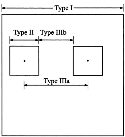
Extent is the total length, area or volume that exists or is observed or analyzed. The extent of the lichen observation portrayed in Fig. 2 is ca 27 cm or 730 cm2. Often, extent is reported in one-dimensional units, though if an area is asymmetrically shaped it is important to describe all dimensions of it. Extent can be unambiguously applied to phenomena, observa-tions or analysis. Figure 3 represents the simplest view of observational extent (Type I) as the length of the longest axis of the study domain. It is worthwhile to consider the extent of an analysis when designing the sample, since as mentioned above, the extent of an analysis and the extent of a set of observations are not necessarily the same.
Grain
Grain can also be defined for phenomena, observa-tions and analysis. In the lichen example, the grain of the phenomenon could be defined as the average size of the tiles (Dale 1999), a parameter of the tile size
Fig. 3. A simplified view of observation extent (Type I), grain (Type II) and lag (Type III). Note that Type IIIb=Type IIIa−Type II when units have the same size and shape.
distribution and clearly a property of the structure of the mosaic. There are many examples where grain is used to refer to some property of a phenomenon (Kotliar and Wiens 1990, Gross et al. 1995, Garrett and Dixon 1997, Kaspari and Weiser 1999). It is also often defined as a property of the observations. Leg-endre and LegLeg-endre (1998) state that ‘‘grain size is the size of the elementary sampling units. It may be expressed as the diameter, surface or volume of the matter supporting the measurements.’’ Figure 3 repre-sents a simple view of observational grain (Type II) as the length of one side of a square quadrat used to collect data. Bjornstad et al. (1999) also use a defini-tion tied to the observadefini-tions, distance to the nearest sampling unit (a definition which seems closer to that of ‘‘lag’’ – see below). Costanza and Maxwell (1994) define it as the smallest unit of measure. Dutilleul (1998) says it is the finest distinction that can be made between two sampling units and equates this with the geostatistical concept of support (see below). Analysis grain may differ from the sampling unit grain if sampling units are aggregated into larger units. The lack of consensus on the precise meaning of grain suggests that an explicit definition of grain is needed when it is used.
Resolution
of the smallest sampling unit or grain size of its sam-pling design (Schneider 1994, Gustafson 1998). This definition, based strictly on the spatial aspects of the sampling unit, ignores the crucial element of the at-tribute (z) measurement scale (Perry et al. 2002). Let us assume that the lichen in Fig. 2 are all various shades of green. Suppose that an image taken of the lichen had a radiometric sensitivity only great enough to read ‘‘green’’ or ‘‘not-green.’’ Lichen species com-prising the various tiles could not be resolved, no matter how small the size of the image grid cells. Therefore, resolution involves more than observation grain alone. This point has generally been ignored in the literature.
Lag
Lag refers to the spacing or interval between neigh-boring unit phenomena or neighneigh-boring sampling or analysis units. Unless clearly defined, there are a few possible interpretations of the word in either measure-ment or analysis. Figure 3 shows that lag may refer to the distance between the centroids of the sampling units (Type IIIa) or the distance between the closest boundaries of the sampling units (Type IIIb).
Support
The geostatistical concept of support belongs on the analysis axis of scale, in that it is a property of a variable used to model data. The support can be as small as a point or as large as the full extent of the spatial field. The spatial unit used to sample the envi-ronment has also been considered the support of the data (Rossi et al. 1992).
A change in any characteristic of the support defi-nes a new variable. This was the fundamental insight of the geostatisticians. A variable, say organism abun-dance, measured on one support is a different vari-able than the same organism’s abundance measured on a different support. The usual geostatistical nota-tion would symbolize these as Zv1(x) and Zv2(x), where v1 and v2are the two distinct supports. It may seem intuitive to suggest that a variable is defined by attribute alone (i.e. organism abundance, species pres-ence/absence, vegetation greenness, etc.), but the spa-tial aspects of the sampling unit are also critical. Statistically, the same attribute measured using two different sampling units must define different variables because they have different distributions. The first-or-der characteristics (the central tendencies) of these distributions may be the same, but their second-order (such as the variance) and higher-order statistics al-most certainly are not.
Cartographic ratio
When ecological data are presented or stored as a map, there is a ratio between the distance on the map to the real-world distance that it represents. For the lichen example, that ratio can be calculated from the scale bar beneath the diagram (Fig. 2). Scale as a cartographic ratio has been a fundamental tool for geographers (Silbernagel 1997). The larger the scale, the larger the value of this ratio. A typical ratio, one cm to the kilometer (1:100000) is thus a smaller scale than 1:24000. Typically, larger scales in this sense represent smaller extents, though this is not always the case. As the mosaic in the diagram has a cartographic ratio fairly close to 1:1, we would say it is a large-scale diagram, despite the fact that it represents an extent of only 27 cm. This geographic meaning of scale refers only to the cartographic representation of the world, not the phenomena being studied or the observations made of them. Ecologists often use ‘‘large scale’’ to refer to large extents and ‘‘small scale’’ to refer to small extents of phenomena, observations or analysis. This usage conflicts with the cartographic usage. Potential confusion because of this conflict can be limited by making the context of scale clear. A simple solution is to avoid the word scale and use extent when appropri-ate (e.g. ‘‘global extent’’ instead of ‘‘global scale’’).
Scale
Scale has been used as a synonym for all of the above-mentioned terms, including their different appli-cations on the phenomenon, observation and analysis axes. In addition there are some related definitions that have been used. For example, the distribution of the means of the tile sizes for each of the s species is used to define the ‘‘scale of pattern’’ of the mosaic. The ‘‘scale of pattern’’ in a multi-species or multi-phase system is one-half the average of the mean distances between tiles of the same phase (Dale 1999). Scale in this context is related to the studied phenomenon. Landscape ecologists define scale as ‘‘grain and extent’’ (Turner 1989, Gustafson 1998). A change of scale in this context may mean a change in grain, a change in extent, or both. Schneider (1994) uses the definition that scale ‘‘denotes the resolution within the range of a measured quantity.’’ A more complicated (and mysteri-ous) definition is, ‘‘a change in pattern as determined by the spatial and or temporal extent of measurements necessary to detect significant differences in the vari-ability of the quantity of interest’’ (Gardner 1998). Given this huge variety of disparate meanings, scale terms must be specific to be understood.
analysis should be considered as separate subjects. The scales of phenomena can only be studied using a choice of scales of observation and analysis – there-fore not all regions within the space defined by the three dimensions in Fig. 3 are possible. Regions that are possible are partly circumscribed by the fact that as the size and shape of the sampling units, the extent of the sample or the lag between sampling units change, inferences about phenomena may change. The next section of this paper focuses on this idea.
Changing observation and analysis scales
influence inference
In ecology, it is well known that observation scales can influence ecological inference (Mercer and Hall 1911, Home and Schneider 1995). The characteristics of a variable’s distribution depend on the area or volume over which it is measured or calculated. Spe-cifically, inference about the population mean and variance, the strength and character of spatial autocor-relation, spatial anisotropy, patch and gap sizes, as well as multivariate relationships are all dependent on the size and shape of sampling units and the lags and extent of sampling. Furthermore, if the size, shape, lag or extent of the analysis is changed, inference can be affected. We now consider specific targets of inference and how they are influenced by changing sampling unit size and extent.
Estimate of the population mean
Many ecological attributes can be expected to average linearly so that the estimate of a population mean will not change if the size of the sampling unit is changed. For example, mean species abundance per unit area can be measured using 1 m2 or 1 ha blocks. Other attributes, those that represent some non-linear func-tion of a quantity, do not have this property. Exam-ples of these attributes are the ph of precipitation samples or the Normalized Difference Vegetation In-dex (NDVI), a ratio of reflectances. That is, the aver-age of NDVIs calculated from 900-m2 pixels is expected to differ from the average of NDVIs calcu-lated from 1.1-km2 pixels covering an identical extent (Aman et al. 1995).
Regardless of the type of attribute, the variance of the mean, which is used to make a statement about the precision of the mean estimate, is expected to change with the size of the sampling unit (Home and Schneider 1995). This leads to advice to choose the largest quadrat size practicable in the sampling design (Kenkel and Podani 1991), since variance is expected to decrease and therefore precision will increase with
increasing quadrat size. With spatially autocorrelated data, this decrease is not as rapid as it would be with independent data. This advice goes counter to the practice of sampling the ‘‘minimum area’’ per unit (Greig-Smith 1983), because that practice is tailored to objectives of measuring spatial pattern rather than es-timating the population mean.
When the extent of a sample is changed, estimates of both the mean value of the population and its precision can be expected to change. Variance could in general be expected to increase, though this is by no means guaranteed.
Estimate of the population variance
Home and Schneider (1995) reviewed the ecological literature on the dependence of variance on ‘‘scale,’’ which in their context most often referred to the size of the sampling unit. In geostatistics, the need for models explaining this dependence arose with require-ments to predict the tonnage of ore realizable by the truckload based on data from the much smaller core or blasthole samples (Journel and Huijbregts 1978, Rendu 1981). These were generally called ‘‘change of support’’ models, explaining the effect that support has on statistics. As support gets larger (also known as regularization), in general, the new variable will have a smaller variance and a more symmetric distribution.
Presence and characteristics of spatial autocorrelation
Along with a decrease in population variance with increasing sampling unit size, changes in pairwise vari-ances are expected. Therefore Moran’s I, Geary’s c, correlograms and semivariograms will change. In many cases, the semivariogram sill and nugget vari-ance will decrease and the range will increase with increasing sampling unit size. These changes were demonstrated empirically by Bellehumeur et al. (1997) and analytically by Bellehumeur and Legendre (1997).
Presence of anisotropy
affected by a specific size change because it is already suffering from a relatively lower sample size than is an isotropic measure of spatial pattern. For example, in a 20×20 grid, there are 79800 pairs of cells to use in the calculation of an omnidirectional spatial mea-sure. Restricting calculations to one direction yields only 3800 pairs. The variance will be hugely affected by this decreased sample size. A sampling unit aggre-gation to a 10×10 grid yields 4950 pairs for the omnidirectional measure, but only 450 for one direc-tion. There is a much greater percentage decrease for the omnidirectional measure, but the sample size is so much smaller for the directional measure that its in-crease in variance will have a more profound effect.
Patch and gap size
Fortin (1999) considered differences in lag distances and quadrat size and shape. In her complete survey of the abundances of three plant species collected in contiguous 5×5 m quadrats within a 60×140 m ex-tent, she found that quadrat sizes smaller than the identified patch size made little difference to patch size inferred from Moran’s I correlograms. Various lag distance classes did not change the conclusions. With other data sets, as we will see in the case stud-ies section, this is not always the case.
Multivariate relationships
Given the effects on inference that we have discussed with a change in the spatial characteristics (size, shape, lag and extent) of sampling units of a single variable, it follows that if the unit sizes of two or more variables change, their covariance and correla-tion statistics also change. Pearson and Carroll (1999) found an ecological example of this effect in the bivariate relationship between bird and butterfly counts over the western United States. The relation-ship changed when the grid cell was quadrupled (from 137.5-km cells to 275-km cells). This effect in multivariate data has been identified in the geography literature as the ‘‘modifiable areal unit problem,’’ or MAUP (Openshaw 1984). The MAUP is not a recent discovery (Gehlke and Biehl 1934) but it became an active area of research in geography in the 1980s. It states that changing the shape and/or size of the units on which data are mapped can change the resulting correlations or statistical models generated from the data. Openshaw (1984) distinguished the ‘‘zoning’’ (changing shape) from the ‘‘aggregation’’ (increasing size) components of the problem. Jelinski and Wu (1996) recognized that this problem can occur with ecological data.
Predicting the effects of observation and analysis scale changes
Can any of the above changes in inference be predicted a priori? Classical statistical theory provides the basis for predicting a change in variance, for independent sampling units, with increasing sampling unit size. Given that most ecological variation is spatially depen-dent, geostatistical regionalized variable theory can be expected to be more accurate in predicting variance than theory based on independent sampling units. In addition, geostatistical theory can predict changes in spatial autocorrelation. Bellehumeur and Legendre (1997) apply this theory to accurately predict the vari-ance, sill, range and nugget variance of tree density at two different sampling unit sizes given measurements on a third sampling unit size. However, the effects of sampling unit shape as well as the effects of extent and lag are not likely to be as predictable. More generally, a solution to the MAUP is elusive, but King (1997) has shown that statistical results can at least be bounded. King’s findings have yet to be applied to ecological data. If ecologists are explicit about all of the compo-nents and dimensions of scale so that the spatial char-acteristics of the quantities measured can be correctly interpreted, there will be new opportunities to gain experience and improve understanding of the effects of observations and analysis scale changes.
Case studies
We have seen that the choices investigators have to make in the design of the sample and in the statistical analysis done on the data can affect the scales of the phenomena that are detected or quantified in the results of analysis. In this section, we give concrete illustra-tions, with several censused data sets, showing how these choices influence outcomes.
Four case studies are examined where data are all point-referenced (Perry et al. 2002) and represent com-plete censuses within a given extent. The data consist of percent cover of Betula glandulosaand counts of Am
-brosa dumosa, isopod burrows and Nyssa aquatica
et al. 1993). Two of these four data sets are further described in Perry et al. (2002). The grid cell sizes, extents and lags were changed in these case studies. Each change considered (whether an increase in unit size, an increase in lag or a decrease in extent) results in a reduction in the number of samples, n. Relative to the complete data set, the changed sets have their sample size reduced from four- to 75-fold. A brief summary of each complete set is documented in Table 1, with its spatial pattern prior to the change in sampling, the form of the change and the effect of the change.
The analysis used in each example includes at least one of the methods designed to detect and describe spatial pattern (e.g. see Perry et al. 2002). These meth-ods include ‘‘variography’’, wherein semivariograms are calculated from the data and their shapes are inspected or modelled (Rossi et al. 1992). Ripley’s K and L methods (Ripley 1981), and SADIE (Spatial Analysis by Distance Indices). SADIE is a class of methods designed to detect clusters, either patches or gaps (Perry et al. 1999). The calculations (Dale et al. 2002) involve comparisons of local density with those elsewhere made across the whole study arena simultaneously. Each sampling unit is assigned an index of clustering and the overall degree of clustering into patches and gaps is assessed by a randomization test.
Change in unit size and shape
Consider two sampling unit sizes, v1Bv2. If the major process affects regions larger than v2, then use of v2 may impair the detection of pattern compared to the use of v1. However, if the process affects regions of sizes between v1and v2, then the pattern found may be qualitatively different.
To illustrate the first outcome, consider a change in unit size from 25 to 100 m2achieved by aggregating the counts of plants in groups of four contiguous grid cells for the Ambrosia dumosa counts (Table 1). Similar weakening in detection resulted for both SADIE (Table 2) and variography (Fig. 4) methods. For SADIE, increased unit size led to a loss of the significance of the strong pattern and a reduction in the definition of clusters, although cluster size was not affected greatly. The semivariogram was more variable for the larger unit size, spatial structure appeared weaker and the estimated range increased from 15 to 25 m.
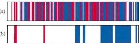
To illustrate the second outcome, consider a change in unit size from 0.01 m2, through 0.04 to 0.08 m2by aggregation of contiguous transect units into groups of first four, and then eight, forBetula glandulosa% cover (Table 1). SADIE revealed extremely strong clustering (pB0.0005) with the smallest unit size, with mean values of indices over three times that expected for a random pattern. A large range of patch sizes were detected, including many small ones. The 73 identified
patches ranged from 0.01 to 0.17 m2with mean 0.040 m2; the 106 gaps ranged from 0.0l to 0.33 m2with mean size 0.030 m2 (Fig. 5a). The degree of pattern and number of clusters identified was qualitatively different when unit size was increased to 0.04 m2(Table 1). Note that the mean cluster sizes for patches and gaps found for the smallest unit size of 0.01 m2were both less than for the largest unit size studied, 0.08 m2. At this largest unit the measured pattern was indistinguishable from random (p\0.05). Fewer clusters were identified; only two patches, both \0.1 m2, and only five gaps, again of relatively large size, ranging from 0.11 up to 1.2 m2 (Fig. 5b).
Another example of the effect of an increase in unit size was calculated for the isopod burrow count data (Table 1). The increase, from 25 m2in the first case to 625 m2in the second, represents a 25-fold change. Both unit sizes resulted in the identification of strong spatial structure, similar sills and ranges of ca 125 m (Fig. 6). The semivariogram of the smaller units could be mod-eled with nested models with various ranges shorter than 125 m, but the semivariogram of the larger units appears to coincide well with a single-range model. The shorter ranges (which are not deterministically deriv-able from the semivariogram alone) seem to disappear from this second semivariogram.
Change in lag
Similar outcomes are expected from a change in lag as from a change in unit size and again the effect depends on the relationship between the size of the region affected by the major process and the comparative lag values studied. For a fair comparison with the change in unit size in the A. dumosa data, described above, a two-fold increase in lag was studied, since the effect of this was, once again, to decrease n from 400 to 100 (Table 1). Broadly, the result from SADIE analysis for the change in lag was indeed similar to that from the change in unit size described above; there were fewer identified clusters and a weakened conclusion. Note that for the above set, and indeed for any square sampling grid, there were four entirely independent sets of data that might have been chosen to illustrate changes in lag. For example, instead of units separated by 10 m at coordinates: (7.5, 2.5), (7.5, 12.5), (17.5, 2.5), (17.5, 12.5)…, the following could equally well have been chosen: (2.5, 2.5), (2.5, 12.5), (12.5, 2.5), (12.5, 12.5)…. The choice is wholly arbitrary.
Change in extent
634
ECOGRAPHY
25:5
Table 1. Summary of the effect of changes in extent (E), lag (L) or unit size (S) on three data sets, exemplified by three methods. Relative to the complete data set, the changed sets with smaller n are reduced in sample size, from four- to 75-fold.
Spatial pattern of changed set
Changed set Change in sampling
Complete set
Dataset Methods
parameters and spatial pattern
Extent
n=20×20=400 Variograpphy,
A.dumosacounts (1) n=10×10=100 no spatial covariance; appears random no clustering; appears random SADIE
E=100×100 m=1 ha E=25×25 m=0.25 ha
clusters smaller and lack definition; SADIE
Lag (2) n=10×10=100
S=5×5 m=25 m2
L=5 m L=10 m pattern weaker
Variography, pattern weaker; variographic range ca 25 Unit size
(3) n=10×10=100 strong pattern; variographic
S=10×10 m=100 m2 SADIE m
range ca 15 m; clusters up
pattern non-significant; clusters lack to ca 450 m2
definition
moderate and significant pattern; 10 n=1001×1=1001 (1) n=250×1=250 Unit size
B.glandulosacounts SADIE
S=0.4×0.1 m=0.04 m2 clusters only
E=10.01 m2
S=0.1×0.1 m=0.01 m2
L=0.1 m
some pattern, but non-significant; 7 very strong spatial pattern; (2) n=125×1=125 Unit size SADIE
clusters only, some increased in size 107 clusters identified S=0.8×0.1 m=0.08 m2
strong pattern; same variographic range n=3024
Isopod burrow counts n=120 Unit size Variography
of ca 125 m E=7.56 ha S=25×25 m=625 m2
S=5×5 m=25 m2
L=5 m
very strong pattern; vario-graphic range ca 125 m
completely indistinguishable from random
Isopod burrows; n=2015 (1) n=59 Extent Ripley’s K
E=75 600 m2 E=14.6×6.6=96.4 m2
mapped individuals
Ripley’s K moderately and significantly aggregated Extent
intense aggregation (2) n=2
Table 2. The effect of changes in extent (E), lag (L) and unit size (S) on revealed spatial pattern of counts ofA.dumosaanalyzed by SADIE.
Set mean cluster index (p) max. cluster size (m2)
gap
Patch gap patch
Complete 1.29 (0.048) −1.35 (0.025) 270 450
Quarter extent 0.98 (0.49) −1.05 (0.32) 75 105
Doubled lag 1.09 (0.24) −1.22 (0.088) 105 420
Unit size increased four-fold 1.13 (0.20) −1.15 (0.17) 300 425
the region affected by a process is larger than or approximates a changed extent, then a considerable change in the perceived pattern is expected, and all pattern might be lost. Three data sets are used to exemplify the effects of a change in extent.
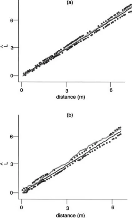
For a fair comparison with the above changes in unit size and lag for the A. dumosa data, a four-fold de-crease in extent was studied that once again reduced sample size, n, from 400 to 100 (Table 1). In this case, it was the upper-left quarter (xB50; y\50) of the original set that was chosen for study, but, as discussed above, the choice of precisely how to reduce extent was arbitrary. A complete absence of pattern was found both by the SADIE (Table 2) and the variography (Fig. 4) methods; neither method could support an inference that the area studied formed part of a larger and significantly non-random pattern. Interestingly, had the lower-left quarter been chosen, the reduction in sample size would not have prevented the detection of pattern. While changes of unit size and lag are not relevant to mapped-individual data, a change of extent may be. The second example concerns the mapped isopod bur-row data (Table 1). The complete data set (Fig. 7) clearly is strongly aggregated. Subsets with lesser extent may show any degree of pattern. Even subsets defined by very closely separated extents may yield completely different patterns, ranging from random (Fig. 7, right insert) to aggregated (Fig. 7, left insert) when measured by standard distance techniques such as Ripley’s L. method (Fig. 8) (Ripley 1981, section 8.3).
A third example illustrates the effect of a change of extent on the measurement of spatial association be-tween two spatial patterns. The complete set of the locations of male and female Nyssa aquatica trees, described previously by Shea et al. (1993), was sampled using two different extents to produce two different maps (Fig. 9). The lower map is an almost complete subset of the upper and has considerable overlap with the region labelled AB of the latter. Now, consider the degree of spatial association between the male and female trees. In the upper map of Fig. 9, there appears considerable positive association between the genders. This may be a real and direct effect, by virtue of a biological process siting males close to females or
vice-versa. Alternatively, it may be nothing more than an artifact caused by the relationship of both genders with some third, unseen variable, such as water depth. In that case, it may be that both genders of tree require some minimum depth of water, which may not be available all over the sampled area. Then, the spatial
Fig. 4. Semivariograms for Ambrosia dumosacounts/unit. complete data set (n=400; extent (E)=1 ha; unit size (S)=25 m2),extent reduced to E
=0.25 ha and×unit size increased to S=100 m2.
Fig. 5. SADIE cluster maps forBetula glandulosaat two unit sizes along a line transect, (a) map from complete data set, n=1001, extent (E)=10.01 m2, unit size (S)=0.1×0.1 m= 0.01 m2. Red shading indicates patches with cluster index values\1.5; blue shading indicates gaps with index valuesB
−1.5; white areas represent lengths that are neither patches nor gaps, (b) map from reduced data set, n=125, E=10.01 m2, S
Fig. 6. Two semivariograms for isopod burrows. complete data set: n=3024, E=7.56 ha, S=5×5 m=25 m2 with ordinate on the left vertical axis and maximumg=0.048. reduced data set: unit size increased to S=25×25 m=625 m2, n=120 with ordinate on the right vertical axis and maximum
g=0.54.
Given the range of outcomes possible, it is important to make a considered choice of the phenomena that will be studied so that the unit sizes and shapes, lags and extents of data collection and analysis can be intelligently chosen and clearly communicated. Ecologists have his-torically and routinely done this, but have not necessarily made these decisions explicit. Making definitions clear can help formalize the process and reduce chances of misinterpretation. In the next section, we discuss the implications to sampling design.
Considerations of observation scale in
sampling design
Ecological sampling has to be carried out using sampling unit sizes, shapes, lags and extents that are
appro-Fig. 8. Graphs of Ripley’s L. versus inter-point distance (m) for (a) left subset; and (b) right subset from Fig. 7. Envelopes of upper and lower 2.5% prediction limits for randomized values as symbols, smoothed median randomized values as black line and observed values as gray line. Significant aggregation is indicated where the gray line breaks out of the envelope. Fig. 7. Map of complete isopod burrow data set with n=2015
individual burrows and extent (E)=75600 m2. Inset maps show two subsets with reduced rectangular extent, both with E=
14.6×6.6 m=96.4 m2. The two subsets are separated by only 8 m. The first (right inset) contained 59 individuals in a pattern indistinguishable from random; the second (left inset to left) contained 27 individuals in a significantly aggregated pattern.
association is an indirect effect, which is apparent only because there are relatively large areas of the upper map in which neither males nor females occur. The problem of identifying which process is responsible is possible only by examining the data at some reduced extent.
Fig. 9. MappedNyssa aquaticatrees from Shea et al. (1993); females are represented as open circles and males are repre-sented as filled circles. The two rectangular areas shown both represent subsets with reduced extent, each part of a larger ca 50×50 m sample. The lower area overlaps considerably with the region labelled AB of the upper area.
objects or processes?’’ and ‘‘What is the spatial pattern of the distribution of these objects or processes?’’
To answer these questions, the spatial scale compo-nents of the sampling design have to allow detection of the patterns that may exist in the study area. Data obtained from the literature or from a pilot study form the basis for appropriate decisions. A well-focused question generally reduces the difficulty of choosing the type of sampling design (simple random, systematic, stratified, etc.) as well as its scale components (size, shape, lag, extent).
The following guidelines, reworked from Legendre and Legendre (1998), are critical in the design of a field survey or experiment:
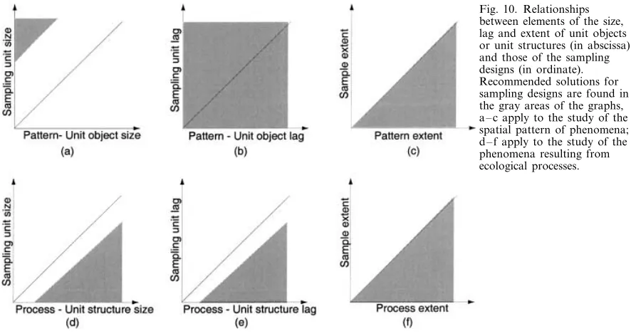
1) The size of the sampling units should be larger than a unit object (e.g., an individual organism; Figs 10a and 11a). It should be large enough to contain at least a few, and preferably several, unit objects. Sam-pling units designed in this way obtain counts instead of presence-absence data. In turn, counts allow the use of methods of surface pattern analysis which assume that the underlying quantitative variation is continuous. 2) The size of the sampling units should be smaller than the structures resulting from the unit process (e.g., a patch) that one is hoping to detect through the sampling design (Figs 10d and 11b). An equivalent concept is found in space or time series analysis, where the shortest period (for time series) or wavelength (for spatial transects) that can be resolved in periodic analy-sis is twice the interval between successive observations; the inverse of this value is called the Nyquist frequency. 3) The spatial lag for analysis of a pattern is a function of the sample size (n) which, inturn, depends upon the total effort allowable for the study (Fig. 10b). Once the sampling unit size has been determined, the relationships of n to lag and extent are
lag=extent
n (along a transect), (1)
lag=
extent 2n
1/2
(on a surface), (2)
lag=
extent 3n
1/3
(on a volume). (3)
In other words, for fixed extent, the spatial lag de-creases when n inde-creases. Prior to a field study, one should check that n provides enough power for detect-ing the hypothesized pattern, given the anticipated size of the effect; see Legendre et al. (2002). n may also be constrained by the method chosen for statistical analy-sis, some methods being more data-hungry than others. 4) The sampling lag (or spacing) should be smaller than the average distance between the structures result-ing from the hypothesized process (Fig. 10e). Otherwise one may fail to recognize the structures (e.g., patches) as separate from one another. Sampling designs with priate to detect the patterns or processes one is looking
Fig. 10. Relationships between elements of the size, lag and extent of unit objects or unit structures (in abscissa) and those of the sampling designs (in ordinate). Recommended solutions for sampling designs are found in the gray areas of the graphs, a – c apply to the study of the spatial pattern of phenomena; d – f apply to the study of the phenomena resulting from ecological processes.
varying spatial lags allow the detection of structures of different sizes after a smaller total effort (n) than would be required, for instance, by simple random or system-atic sampling (Fortin et al. 1989).
5) The sampling extent may be at least as large as the total area covered by the type of objects or process under study (Fig. 10c, f). To understand the extent of a structure or process it is of course preferable to sample beyond the boundaries of the phenomenon. For con-stant n, the sampling extent can be maximized by turning the sampling area into a transect, or two or more crossing transects if anisotropy is expected.
Ultimately, no structure can be detected which is smaller than the size of the sampling unit or larger than the extent of a study. Wiens (1989) compares these to the overall size and mesh size of a sieve, respectively.
Conclusion
An interesting dichotomy advanced by Pickett et al. (1994) is ‘‘thing ecology’’ and ‘‘stuff ecology.’’ The former includes portions of the discipline that focus on discrete object-like entities with recognizable spatial boundaries whereas the latter focuses on pools and fluxes of materials and energy. Stern (1998) makes a similar distinction between ‘‘Eulerian’’ and ‘‘Lagran-gian’’ methods in ecology. Eulerian methods, when the unit of study is an area, seem appropriate for stuff ecology and Lagrangian methods, when the unit of study is an individual, are suited to thing ecology. We find that support effects and other scaling issues are particularly relevant to stuff ecology, where the defini-tion of the unit of study is not fixed. Notably,
tics was developed fundamentally for predicting stuff – in this case stuff was defined as metal ore – and it is for stuff ecology that it finds its application.
Because they are often dealing with stuff rather than things, ecologists are faced with the difficult problem of deciding what sampling and analysis units to select, in some cases wholly arbitrary decisions. Much like power calculations are used to decide the number of sampling units, but require some pre-experimental knowledge of variance, decisions of sampling unit size require some idea of the size, spacing and extent of the phenomena that are of interest prior to the data collection effort. Exploratory pilot studies and detailed information on historical sampling schemes, or at the very least hy-potheses about these characteristics, are vital.
The results of our consideration of the myriad mean-ings of scale in ecology have convinced us that there is not one ‘‘problem of scale’’ (Levin 1992), but many, each of which deserves consideration in its own right. Peters (1992) complained about non-operational terms in ecology. ‘‘The terms in good theories are sufficiently well defined or generally known so that most practi-tioners agree about which theoretical variables repre-sent which phenomena’’ (Peters 1992, p. 30). We argue that to make theories about ‘‘scale’’ operational, its specific components relevant to observation, phenom-ena and analysis should be spelled out. We urge ecolo-gists to be explicit on their usage of the term scale and to report the decisions that were implemented in the sampling design and in the statistical analysis.
Acknowledgements – The work reported in this paper was conducted as part of the Working Group Integrating the Statistical Modeling of Spatial Data in Ecology by the Na-tional Center for Ecological Analysis and Synthesis (NCEAS), a Center funded by NSF (GrantcDEB-94-21535), the Univ. of California at Santa Barbara and the State of California.
References
Aman, A. et al. 1995. Upscale integration of Normalized Difference Vegetation Index: the problem of spatial hetero-geniety. – IEEE Trans. on Geoscience and Remote Sensing 30: 326 – 337.
Bellehumeur, C. and Legendre, P. 1997. Aggregation of sam-pling units: an analytical solution to predict variance. – Geogr. Anal. 29: 258 – 266.
Bellehumeur, C., Legendre, P. and Marcotte, D. 1997. Vari-ance and spatial scales in a tropical rain forest: changing the size of sampling units. – Plant Ecol. 130: 89 – 98. Bjornstad, O. N., Stenseth, N. C. and Saitoh, T. 1999.
Syn-chrony and scaling in dynamics of voles and mice in northern Japan. – Ecology 80: 632 – 637.
Costanza, R. and Maxwell, T. 1994. Resolution and pre-dictability – an approach to the scaling problem. – Land-scape Ecol. 9: 47 – 57.
Csillag, F., Fortin, M.-J. and Dungan, J. L. 2000. On the limits and extensions of the definition of scale. – Ecol. Soc. Am. Bull. 81: 230 – 232.
Dale, M. R. T. 1999. Spatial pattern analysis in plant ecology. – Cambridge Univ. Press.
Dale, M. R. T. and Zbigniewicz, M. W. 1997. Spatial pattern in boreal shrub communities: effects of peak in herbivore densities. – Can. J. Bot. 7: 1342 – 1348.
Dale, M. R. T. et al. 2002. Conceptual and mathematical relationships among methods for spatial analysis. – Ecog-raphy 25: 558 – 577.
Dutilleul, P. 1998. Incorporating scale in ecological experi-ments: data analysis. – In: Peterson, D. L. and Parker, V. T. (eds), Ecological scale: theory and methods. Columbia Univ. Press, pp. 369 – 386.
Ehleringer, J. R. and Field, C. B. 1993. Scaling physiological processes: leaf to globe. – Academic Press.
Fortin, M.-J. 1999. Effects of quadrat size and data measure-ment on the detection of boundaries. – J. Veg. Sci. 10: 43 – 50.
Fortin, M.-J., Drapeau., P. and Legendre., P. 1989. Spatial autocorrelation and sampling design in plant ecology. – Vegetatio 83: 209 – 222.
Gardner, R. H. 1998. Pattern, process and analysis of spatial scales. – In: Peterson, D. L. and Parker, V. T. (eds), Ecological scale. Columbia Univ. Press, pp. 17 – 34. Gardner, R. H. et al. (eds) 2001. Scaling relations in
experi-mental ecology. – Columbia Univ. Press.
Garrett, K. A. and Dixon, P. M. 1997. Environmental pseu-dointeraction: the effects of ignoring the scale of environ-mental heterogeneity in competition studies. – Theor. Popul. Biol. 51: 37 – 48.
Gehlke, C. E. and Biehl, K. 1934. Certain effects of grouping upon the size of the correlation coefficient in census tract material. – J. Am. Stat. Assoc. 29: 169 – 170.
Greig-Smith, P. 1983. Quantitative plant ecology. – Univ. of California Press.
Gross, K. L., Pregitzer, K. S. and Burton, A. J. 1995. Spatial variation in nitrogen availability in three successional plant communities. – J. Ecol. 83: 357 – 367.
Gustafson, E. 1998. Quantifying landscape spatial pattern: what is the state of the art? – Ecosystems 1: 143 – 156. Home, J. K. and Schneider, D. C. 1995. Spatial variance in
ecology. – Oikos 74: 18 – 26.
Jelinski, D. E. and Wu, J. G. 1996. The modifiable areal unit problem and implications for landscape ecology. – Land-scape Ecol. 11: 129 – 140.
Jenerette, G. D. and Wu, J. 1999. On the definitions of scale. – Ecol. Soc. Am. Bull. 1: 104 – 105.
Journel, A. G. and Huijbregts, C. J. 1978. Mining geostatis-tics. – Academic Press.
Kaspari, M. and Weiser, M. D. 1999. The size-grain hypothe-sis and interspecific scaling in ants. – Funct. Ecol. 13: 530 – 538.
Kenkel, N. C. and Podani, J. 1991. Plot size and estimation efficiency in plant community studies. – J. Veg. Sci. 2: 539 – 544.
King, G. 1997. A solution to the ecological inference problem. – Princeton Univ. Press.
Kotliar, N. B. and Wiens, J. A. 1990. Multiple scales of patchiness and patch structure: a hierarchical framework for the study of heterogeneity. – Oikos 59: 253 – 260. Legendre, P. and Legendre, L. 1998. Numerical ecology. –
Elsevier.
Legendre, P. et al. 2002. The consequences of spatial structure for the design and analysis of ecological field surveys. – Ecography 25: 601 – 615.
Levin, S. A. 1992. The problem of pattern and scale in ecology. – Ecology 73: 1943 – 1967.
Mercer, W. B. and Hall, A. D. 1911. The experimental error of field trials. – J. Agricult. Sci. 4: 107 – 132.
Miriti, M., Howe, H. F. and Wright, S. J. 1998. Spatial patterns of mortality in a Colorado desert plant commu-nity. – Plant Ecol. 136: 41 – 51.
Norowi, H. M. et al. 2000. The effect of spatial scale on interactions between two weevils and their parasitoid. – Ecol. Entomol. 25: 188 – 196.
Openshaw, S. 1984. Concepts and techniques in modern geog-raphy number 38: the modifiable areal unit problem. – GeoBooks.
Pearson, D. L. and Carroll, S. S. 1999. The influence of spatial scale on cross-taxon congruence patterns and prediction accuracy of species richness. – J. Biogeogr. 26: 1079 – 1090. Perry, J. N. et al. 1999. Red-blue plots for detecting clusters in
count data. – Ecol. Lett. 2: 106 – 113.
Perry, J. N. et al. 2002. Illustrations and guidelines for select-ing statistical methods for quantifyselect-ing spatial patterns in ecological data. – Ecography 25: 578 – 600.
Peters, R. H. 1992. A critique for ecology. – Cambridge Univ. Press.
Peterson, D. L. and Parker, V. T. 1998. Dimensions of scale in ecology, resource managements and society. – In: Peter-son, D. L. and Parker, V. T. (eds), Ecological scale: theory and methods. Columbia Univ. Press, pp. 387 – 425. Pickett, S. T., Kolasa, J. and Jones, C. G. 1994. Ecological
understanding. – Academic Press.
Rendu, J.-M. 1981. An introduction to geostatistical methods of mineral evaluation. – South African Inst. of Mining and Metallurgy, Johannesburg, South Africa.
Ripley, B. D. 1981. Spatial statistics. – Wiley.
Rossi, R. E. et al. 1992. Geostatistical tools for the modeling and interpretation of ecological spatial dependence. – Ecol. Monogr. 62: 277 – 314.
Schneider, D. C. 1994. Quantitative ecology: spatial and tem-poral scaling. – Academic Press.
Shea, M. M., Dixon, P. M. and Sharitz, R. R. 1993. Size differences, sex ratio and spatial distribution of male and female water tupeloNyssa aquatica(Nyssaceae). – Am. J. Bot. 80: 26 – 30.
Silbernagel, J. 1997. Scale perception-from cartography to ecology. – Ecol. Soc. Am. Bull. 78: 166 – 169.
Stern, J. S. 1998. Field studies of large mobile organisms: scale, movement, and habitat utilization. – In: Peterson, D. L. and Parker, V. T. (eds), Ecological scale: theory and methods. Columbia Univ. Press, pp. 289 – 307.
Turner, M. G. 1989. Landscape ecology: the effect of pattern on process. – Annu. Rev. Ecol. Syst. 20: 171 – 197.