University of New Orleans University of New Orleans
ScholarWorks@UNO
ScholarWorks@UNO
University of New Orleans Theses and
Dissertations Dissertations and Theses
Fall 12-18-2014
Investigation of the Quenching Characteristics of Steel
Investigation of the Quenching Characteristics of Steel
Components by Static and Dynamic Analyses
Components by Static and Dynamic Analyses
Pratik Sarker [email protected]
Follow this and additional works at: https://scholarworks.uno.edu/td
Part of the Applied Mechanics Commons
Recommended Citation Recommended Citation
Sarker, Pratik, "Investigation of the Quenching Characteristics of Steel Components by Static and Dynamic Analyses" (2014). University of New Orleans Theses and Dissertations. 1942.
https://scholarworks.uno.edu/td/1942
This Thesis is protected by copyright and/or related rights. It has been brought to you by ScholarWorks@UNO with permission from the rights-holder(s). You are free to use this Thesis in any way that is permitted by the copyright and related rights legislation that applies to your use. For other uses you need to obtain permission from the rights-holder(s) directly, unless additional rights are indicated by a Creative Commons license in the record and/or on the work itself.
Investigation of the Quenching Characteristics of Steel Components by
Static and Dynamic Analyses
A Thesis
Submitted to the Graduate Faculty of the University of New Orleans in partial fulfillment of the requirements for the degree of
Master of Science in
Engineering-Mechanical Solid Mechanics
by
Pratik Sarker
B.Sc., Bangladesh University of Engineering and Technology, 2007
ii
DEDICATION
To
My Father
who taught me never to lose hope and always try to the end without expecting anything for
earning an honest living
and
My Mother
who always encouraged me to listen to my mind to do things as I think is good and to have faith
iii
ACKNOWLEDGMENT
First of all, I would like to express my sincere gratitude to my advisor, Dr. Uttam K
Chakravarty for the continuous support of my Master’s study and research, for his patience,
motivation, enthusiasm, and immense knowledge. I am especially thankful for his guidance on
fostering my professional problem-analyzing, problem-solving, and reporting skills. His
guidance helped me in all the time of research and writing of this thesis.
Besides my advisor, I would like to thank the rest of my thesis committee; Dr. Paul J
Schilling and Dr. Martin J Guillot for their encouragement, insightful comments, and hard
questions. I am also grateful to Dr. Kazim M Akyuzlu and Dr. David Hui for their valuable
advice and guidance.
I thank my fellow labmates in University of New Orleans Computational Solid
Mechanics Group; Manohar Chidurala and Jose Enrique Rubio for the stimulating discussions,
for the sleepless nights we worked together before deadlines, and for all the fun we have had in
the last two years.
Last but not the least, I would like to thank my family; my parents Sribash Chandra
Sarker and Dharitri Sarker for giving birth to me at the first place and supporting me throughout
iv
Table of Contents
List of Figures ... vi
List of Tables ... viii
Abstract ... ix
1. Introduction ... 1
1.1 Scope of Quenching ...1
1.2 Mechanism of Quenching: A typical Heat Treatment Process ...1
1.3 Literature Review...4
1.4 Research Objective ...8
2. Static Quenching Analysis of a Spur Gear ... 10
2.1 Scope of Quenching of a Spur Gear ...10
2.2 Description of the Spur Gear ...10
2.3 Properties of Steel ...11
2.4 Temperature Dependence of the Yield Stress of Steel ...12
2.5 Finite Element Model ...13
2.6 Boundary Conditions ...14
2.7 Mesh Generation ...16
3. Dynamic Quenching Analysis of a Steel Tube... 17
3.1 Scope of Quenching of a Steel Tube...17
3.2 Description of the Steel Tube ...17
3.3 Properties of the Steel Tube ...18
3.4 Properties of the Liquid Quenchants...18
3.5 The Fluid-Structure Interaction Model ...19
3.5.1 General Mathematical Formulation for the CFD Model ...19
3.5.1.1 General Assumptions ...20
3.5.1.2 Conservation of Mass (Continuity Equation) ...20
3.5.1.3 Conservation of Momentum (Navier-Stokes Equations) ...21
3.5.1.4 Conservation of Energy (Energy Equation) ...21
3.5.1.5 Boundary and Initial Conditions ...23
3.5.2 Physical Domain ...25
3.5.3 Interaction ...28
3.5.4 Boundary and Initial Conditions ...28
3.5.4.1 For CFD Model ...28
3.5.4.2 For Solid Model ...30
3.5.5 Mesh Generation ...31
3.5.5.1 For CFD Model ...31
3.5.5.2 For Solid Model ...32
4. Results and Discussions ... 33
4.1 Static Quenching Analysis of a Spur Gear ...33
v
4.1.2 Convergence Study and the Cooling Curve ...34
4.1.3 Stress and Deformation Analysis ...35
4.1.4 Time-varying Nodal Stress and Deformation ...36
4.1.5 Path-wise Stress and Deformation ...37
4.2 Dynamic Quenching Analysis of a Steel Tube ...40
4.2.1 Model Validation ...40
4.2.2 Convergence Study and the Cooling Curve ...40
4.2.3 Stress and Deformation Analysis ...42
4.2.4 Time-varying Nodal Stress and Deformation ...45
4.2.5 Distribution of the Axial Stress and Deformation in the Tube ...47
4.2.6 Distribution of the Radial Stress and Deformation in the Tube...49
5. Conclusions ... 52
5.1 Static Quenching Analysis of a Spur Gear ...52
5.2 Dynamic Quenching Analysis of a Steel Tube ...53
References ... 56
vi
List of Figures
Figure 1.1: A sample TTT diagram for plain carbon eutectoid steel
Figure 1.2: A sample TTT diagram with different microstructures
Figure 1.3: Flow chart of numerical modeling
Figure 2.1: Detailed 3-D model of the full spur gear
Figure 2.2: Quarter of a spur gear with the pathway of analysis
Figure 2.3: Mesh of the quarter gear with element size of 0.16 mm
Figure 3.1: Typical boundary conditions in a viscous heat-conducting fluid flow analysis
Figure 3.2: Computational domain for the liquid quenchant
Figure 3.3: Computational domain for the steel tube
Figure 3.4: Half of the tube with locations of paths (AB and CD) and nodes (2, 24, 25, 27, 52,
68, and 2471) of analysis
Figure 3.5: The fluid domain after meshing
Figure 3.6: The steel tube after meshing
Figure 4.1: Variations of the von-Mises stresses at different nodes with degrees of freedom
Figure 4.2: Variations of the nodal temperatures with time
Figure 4.3: Distribution of the von-Mises stress in the quarter gear
Figure 4.4: Distribution of the deformation in the quarter gear
Figure 4.5: Variations of the von-Mises stresses at different nodes with time
Figure 4.6: Variations of the deformations at different nodes with time
Figure 4.7: Variation of the von-Mises stress along the path 39→40
Figure 4.8: Variation of the deformation along the path 39→40
vii
Figure 4.10: Variations of the temperatures of nodes 2, 24, and 2471 with time for water
Figure 4.11: Variations of the temperatures of node 24 with time for different quenchants
Figure 4.12: Distributions of the von-Mises stresses in (a) the steel tube (b) the cross-sectional
half of the tube in the downstream direction of flow
Figure 4.13: Distributions of the von-Mises stresses on outer surface of the tube in (a) the
upstream direction (b) the downstream direction of flow
Figure 4.14: Distributions of the deformations in (a) the steel tube (b) the cross-sectional half of
the tube in the downstream direction of flow
Figure 4.15: Distributions of the deformations on outer surface of the tube in (a) the upstream
direction (b) the downstream direction of flow
Figure 4.16: Variations of the von-Mises stresses of node 24 with time for different quenchants
Figure 4.17: Variations of the deformations of node 24 with time for different quenchants
Figure 4.18: Variations of the von-Mises stresses axially along path AB from node 52 to node 25
Figure 4.19: Variations of the deformations axially along path AB from node 52 to node 25
Figure 4.20: Variations of the von-Mises stresses radially along path CD from node 68 to node
27
viii
List of Tables
Table 2.1: Physical and thermal properties of steel
Table 2.2: Temperature dependent yield stress of steel
Table 2.3: Global coordinates of the nodes in Fig. 2.2
Table 2.4: Boundary conditions for the quarter spur gear
Table 3.1: Properties of the steel tube
Table 3.2: Properties of the liquid quenchants at 25 °C
Table 3.3: Global coordinates of the nodes in Fig. 3.4
Table 3.4: Boundary conditions for fluid domain
Table 3.5: Boundary conditions for solid domain
ix
ABSTRACT
Machine components made of steel are subjected to heat treatment processes for
improving mechanical properties in order to enhance product life and is usually done by
quenching. During quenching, heat is transferred rapidly from the hot metal component to the
quenchant and that rapid temperature drop induces phase transformation in the metal component.
As a result, quenching generates some residual stresses and deformations in the material.
Therefore, to estimate the temperature distribution, residual stress, and deformation
computationally; three-dimensional finite element models are developed for two different steel
components – a spur gear and a circular tube by a static and a dynamic quenching analyses,
respectively. The time-varying nodal temperature distributions in both models are observed and
the critical regions are identified. The variations of stress and deformation after quenching along
different pathways for both models are studied. The convergence for both models is checked and
validations of the models are done.
Keywords:Quenching process; finite element; fluid-structure interaction; temperature
1
1. Introduction
1. 1 Scope of Quenching
The application of quenching, an essential heat treatment process for hardening materials
in industrial and mechanical fields, is continuously increasing worldwide for developing desired
material properties. From industrial sector to most common use of alloy materials in automotive,
aircraft, heavy machineries, transmission systems, engine components, etc., quenching is
involved as a part of the heat treatment process. Highly loaded gears and shafts, such as those in
transport or racing vehicles or a heavy duty power transmission mechanism should have fracture
toughness and fatigue strength values two or three times those of conventional vehicles or
mechanisms to resist failure. Therefore, they need to be quenched to serve the aforesaid purpose.
In military, aircraft, and naval applications quenched steel plates are used for making dies for
extrusions, nozzles, armor plates, tempered steel bars, deep drawn objects, ship hulls, and many
other parts. Likewise, mechanisms that use moving parts where strength and fatigue resistance is
very important, quenching can essentially ensure the necessary material properties.
This work studies heat transfer, residual and thermal stress, and distortion analysis after
quenching of two steel parts – a spur gear and a circular tube by a static and a dynamic analyses,
respectively. The static analysis uses a constant heat transfer coefficient while the dynamic
analysis uses the fluid flow by three liquid quenchants; water, brine, and propylene glycol (PG).
1.2 Mechanism of Quenching: A Typical Heat Treatment Process
Heat treatment is a method mainly used to alter the physical properties such as
2
concentration of a material or a part. Unlike grinding and machining, there is usually no material
removal in heat treatment processes. Typical heat treatment processes include those altering
physical properties, e.g., quenching, tempering, aging, annealing, and normalizing and also those
involving chemical property changes, e.g., carburizing and nitriding.
In material science, quenching is a heat treatment process, in which it is cooled rapidly
from its austenitization temperature. It prevents low-temperature processes such as phase
transformations from occurring by only providing a narrow window of time in which the reaction
is both thermodynamically favorable and kinetically accessible. Quenching is generally done for
metals that are alloyed with small amounts of other metals, mostly done with steels, an alloy of
iron and carbon. The temperature of steel parts from which cooling starts usually ranges from
815–900 °C. The way quenching works to harden steels is by introducing martensite, a very hard
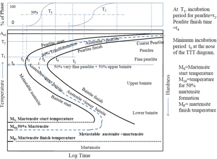
form of steel crystalline structure. Fig. 1.1 shows a schematic time-temperature-transformation
(TTT) diagram [1] for the eutectoid plain carbon steel.
At high temperature, the alloying metals are dissolved in the base metal. If the material is
cooled slowly, the alloy elements have time to precipitate out separately. However, if the metal is
quenched, the alloying metals are trapped within the crystal grains which make it harder. At a
temperature of around 750 °C, iron has a body centered cubic (BCC) structure, called ferrite. The
carbon atoms can easily be held within this less tightly packed structure in what is called a solid
solution. If the steel is cooled slowly, the iron atoms rearrange into a face centered cubic (FCC)
structure, called austenite. The iron atoms are more tightly packed in this arrangement and
cannot hold as many carbon atoms within the structure. The remaining carbon forms a compound
with iron called iron carbide or cementite. If the same steel is quenched rather than being cooled
3
austenite structure in an arrangement called martensite, generated due to the rapid phase
transformation while quenching. The movement of dislocations is very difficult in this structure
so the metal becomes very hard and brittle.
Figure 1.1: A sample TTT diagram for plain carbon eutectoid steel
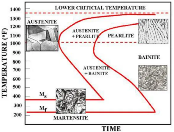
Figure 1.2 illustrates some phases for steel components at different cooling rates. From
Fig. 1.2, martensitic reaction begins during cooling when the austenite reaches the martensite
start temperature Ms and the parent austenite becomes mechanically unstable. As the sample is
quenched, an increasingly large percentage of the austenite transforms to martensite until the
lower transformation temperature Mf is reached, at which the transformation is completed. One
of the differences between the two phases is that martensite has a body centered tetragonal
4
Figure 1.2: A sample TTT diagram with different microstructures
Besides improving mechanical properties, quenching produces some residual stresses in
the material too, which ultimately cause deformations and increase with increasing steel
hardenability. Therefore, it is necessary for the heat treaters to optimize the component design
and the heat treating processes. It is important to note that the hardness is not uniform in the
material after quenching and a hardness gradient exists throughout the material. The final
hardness is dependent on the amount of carbon in the steel. The depth of hardness depends on the
hardenability of the steel as well as the quench severity. The performance capability of the
quenched part is defined by its properties (mechanical, physical, and metallurgical), which are in
turn determined by the part microstructure.
1.3 Literature Review
As quenching is a much accelerated cooling process, it brings the metal back to room
temperature, preventing the lower temperatures through which the material is cooled from
5
quenching rate, the longer the thermodynamic forces have a chance to alter the microstructure,
which is in some cases is desirable. Hence there are uses of different quenching media either
liquids like oil, water, etc., or gases. Elkatatny et al. [2] used a transient flow model aided by
computational fluid dynamics (CFD) to simulate the process of high pressure gas quenching of a
large die in order to predict the temperature distribution. Totten et al. [3] discussed the vapor
blanket and nucleate boiling stage of heat transfer of a hot object when quenched in fluids like
oil or water. Jintang et al. [4] analyzed the quenching process of a heavy rail to obtain the time
varying temperature fields by simulating the different stages of heat treatment using the finite
element software, ANSYS. For a rapid quenching process, the quenchant must produce enough
quench severity to have martensitic transformation. A very common method for that purpose is to
use liquid quenchants. Water and brine [3–7] are two such conventional liquid quenchants used
for rapid cooling. While water quenching results in the formation of hard martensitic
microstructure and subsequently provides high strength and toughness after tempering, it also
has a tendency to create distortion and cracking in the specimen. On the other hand, brine is
somewhat corrosive in nature. Oil quenching does not have these problems, but cannot provide
sufficient cooling rate to harden the part as required to achieve acceptable mechanical properties,
especially in large cross sections. To overcome these disadvantages of quenching by water, brine,
and oil; polymeric solutions are introduced as the substitutions. There are several commercial
polymer quenchants that are readily accepted and used nowadays among which glycol based
quenchants are frequently used [8].
Previous works suggest that the residual stress and deformation are measured by various
methods for conventional and simple geometries in transient stress analysis. Yamada [9]
6
plates with prescribed temperatures. The transient thermal stress problem in a thermally and
elastically orthotropic rectangular slab was investigated by Wang and Chou [10]. Nowadays, the
finite element (FE) method, one of the most powerful numerical methods, is used to predict the
residual and thermal stress in the material. Toparli and Aksoy [5] analyzed the residual stress
developed during water quenching of cylindrical solid steel bars of various diameters using FE
method to find the transient temperature distribution in the bar. Transient temperature and
residual stress fields were carried out by Fa-rong and Shang-li [11] by ADINA/ADINAT
program for a metal specimen during quenching. The commercial FE software, DEFORM-HT
was used to predict the material response for optimizing the gas quenching process in order to
minimize the distortion [12]. Residual stresses in a large circular disk caused by local heating
and cooling at its center was calculated by Gurney [13]. Several researchers [14–17] showed that
the FE method could be used to simulate the real processes by comparing the results with some
experimental data. Numerical investigation of the thermal stress suggested a good validation of
the experimental results [18–19].
The residual stress and deformation created by quenching are influenced by a number of
parameters and vice versa. Sedighi and McMahon [20] investigated the effect of variation in part
orientation and quenchant circulation during quenching of steel parts to estimate the residual
stresses. The residual stress generated after quenching was used to find the impact on fatigue life
in an automotive aluminum alloy by using local stress and idealized pore size in the alloy [21].
Rapid tension tests were performed on the alloy in super-saturated solution state to study the
development of residual stress and deformation during quenching of an aluminum alloy at
several temperatures and strain rates to determine the parameters in the thermo-mechanical
7
accurately in carburized and quenched gear steels to show that distortions were quite sensitive to
small variations in constitutive parameters. The application of new multiphase material model for
simulating deformation and residual stress in carburized and quenched gear steels was also
developed [24]. Different techniques for the measurement of the residual stress like optical strain
rosette, resistance strain rosette, X-ray, neutron diffraction, etc., were used in the experimental
study of residual stress distributions in aluminum castings after water quenching [25].
When quenched, a significant amount of residual stress is developed in the component,
particularly in water [2, 21–22, 26–28] and the relevant previous works suggests some ways to
minimize it. The commercial finite element software, DEFORM-HT, was used to predict the
material response during the quenching process to optimize the gas quenching process in order to
minimize the distortion [12]. Residual stress differences were experimented between water and
air quenched aluminum castings to find significantly reduced residual stress for air quenching
compared to water quenching [28]. Better control over quenching by changing fluid pressure,
speed, flow direction, or the fluid itself enables absolute repeatability, optimized part
microstructure, enhanced mechanical properties, and reduced manufacturing costs. Kavalco et al.
[29] discussed the strength, cooling rate and intergranular corrosion of aluminum alloys with
residual stress or deformation for optimization of the gas quenching efficiency. The heat transfer
coefficient between the hot part and the quenchent affects the quenching result significantly.
Xiao [19] studied the effect of distribution of heat transfer coefficient on the accuracy of thermal
boundary conditions by numerical modeling and experimental investigation for optimization in
quenching processes of aluminum and steel components. Mitchell [30] studied quenching of
wrought 7075 aluminum alloy by calculating the variable heat transfer coefficient to maximize
8
1.4 Research Objective
This work is dedicated to study the thermal behavior and mechanical response of two
different steel parts during the quenching process by static and dynamic analyses. Specifically,
the aims of this work are as follows:
1.Heat Transfer Modeling: At first, the heat transfer model needs to be developed in
order to generate the temperature-time history of the steel part after quenching. In the static
analysis, two different approaches are followed. One is the fully coupled analysis (also called
coupled-temperature-displacement analysis) and another is the sequentially coupled analysis. For
fully coupled analysis, the temperature-time history is developed at an instant and immediately
applied to determine the corresponding stress and deformation at that instant. In the sequentially
coupled analysis, the temperature-time history is developed for the whole part at the first step
and is used as an input to determine the stress and deformation in the second step. In the dynamic
analysis, a fluid-structure interaction (FSI) model is developed and sequentially coupled analysis
is used which uncouples the thermal response from the mechanical response.
2. Stress and Deformation Modeling: The temperature-time history developed in both
the static (sequentially coupled analysis) and dynamic analyses is used to calculate
three-dimensional (3-D) stress and deformation in both steel parts. The time-varying stress and
deformation at a specific point and the variation of stress and deformation along particular
pathways in the steel components are determined.
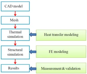
The sequence of the first two steps is summarized more clearly in Fig. 1.3. Results are
obtained after validation of the model is done. The convergence of the results for both analyses
9
Figure 1.3: Flow chart of numerical modeling
3. Identification of the Critical Regions: Once the results are obtained, identification of
the regions of the steel parts in both analyses after quenching is done where the stress and the
deformation are the maximum.
4. Selection of the Proper Quenchant: In the dynamic analysis, the cooling rates for all
the quenchants are compared and the criteria for selecting a suitable quenchant among different
10
2. Static Quenching Analysis of a Spur Gear
2.1 Scope of Quenching of a Spur Gear
Spur gear quenching is done basically to make them suitable for machining into a
particular shape and for withstanding high dynamic stress for a particular service. To control the
deformation and achieve repeatable dimensional tolerances, the gear needs suitable constraints
during the quenching cycle of the heat treatment process. Although heat treating represents a
significant portion (≈ 30%) of a typical gear manufacturing cost, quenching is essentially
important for spur gears to make them harder and tougher as part of the manufacturing process.
This is because spur gears are the most common parts to withstand high dynamic bending and
compressive stresses. They must be capable of resisting frictional wear and should have
enhanced toughness for which sufficient strength is required for better performance and longer
life. To meet all these requirements, the gear must be heat treated. The geometry of the gear is
one of the governing factors to perform well in its service. So, it needs to be in a state or shape in
which minimum amount of residual stress and deformation take place. Therefore, after
quenching, identification of high stress developing regions in the gear is necessary and those
regions need to be carefully designed by considering important design parameters like strength,
cost, durability, and reliability.
2.2 Description of the Spur Gear
The object of analysis here is a steel spur gear and is symmetric about X-, Y-, and Z-axes
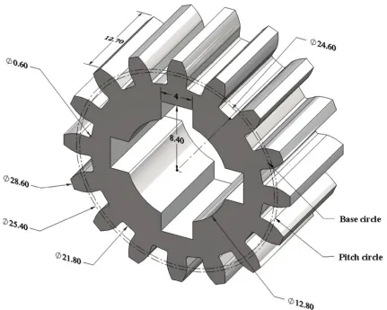
shown in Fig. 2.1. The gear has 16 teeth. The outer circle, pitch circle, base circle, and root circle
diameters are 28.6 mm, 25.4 mm, 24.6 mm, and 21.8 mm, respectively. The height and the
11
Figure. 2.1: Detailed 3-D model of the full spur gear
gear are taken from the Boston gear catalog [31]. All the gear teeth have involute profile and
standard procedures are followed to maintain the involute profile of each tooth using 13 points
[32]. For serving the purpose of an industrial gear, four keyways, symmetric about X-, Y-, and Z
-axes are modeled around the bore hole of the spur gear. The bore diameter is 12.8 mm. The
height of a key slot is 8.4 mm from the center of the bore hole and total width of the key slot is 4
mm. At the root of each tooth, a fillet of radius 0.3 mm is maintained.
2.3 Properties of Steel
The mechanical and thermal properties of steel are given in Table 2.1. It is assumed that
12
Table 2.1: Physical and thermal properties of steel
Material Density, kg/m3 Young’s modulus, Pa Poisson’s ratio Thermal conductivity,
W/m·K
Specific heat, J/kg·K
Coefficient of thermal expansion,
K-1
Steel 7800 207e9 0.3 50 500 0.000013
2.4 Temperature Dependence of the Yield Stress of Steel
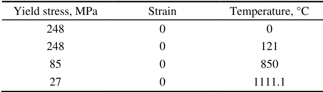
The gear is assumed to be made of an elastic, perfectly plastic steel with the yield stress
that drops linearly with temperature above 121 °C [18]. The transient stress is large enough to
cause significant plastic flow, so residual stress will remain after the plate is cooled to the sink
temperature. The relationship between the temperature dependent yield stress and the
corresponding temperature [18] is given below by the Eqs. 2.1 and 2.2. From Eq. 2.1, when the
temperature of the steel is below or not more than 121 °C, it does not affect the yield stress at all.
But at very high temperature, in general, the yield stress of the steel gets reduced significantly as
indicated by Eq. 2.2. The range of values for the temperature dependent yield stress and the
corresponding temperature for the static model of the gear is described in Table 2.2.
Yield stress, = 248 MPa Temperature, ≤ 121 °C (2.1)
Yield stress, = 248(1 − ( − 121)/1111.1) MPa Temperature, > 121 °C (2.2)
Table 2.2: Temperature dependent yield stress of steel
Yield stress, MPa Strain Temperature, °C
248 0 0
248 0 121
85 0 850
13
2.5 Finite Element Model
Due to the symmetry about the X-, Y-, and Z-axes, a 3-D FE model of the quarter of the
full spur gear is developed for investigating the thermal stress and deformation using the FE
analysis software, Abaqus 6.13 [33]. The analysis is run in a transient mode and in two methods
– the fully coupled and the sequentially coupled analyses. The fully coupled analysis is done by
creating a coupled-temperature-displacement step. In this step, both the heat transfer and the
thermal stress are interrelated. On the other hand, the sequentially coupled analysis is achieved
by two stages; at first, the analysis is run as a pure heat transfer step to get the temperature-time
history until the model is cooled. Secondly, the analysis is completed by creating a static general
step, where the temperature-time history generated from the heat transfer step is given as an
input. In the sequentially coupled analysis, the pure heat transfer step is done without setting any
mechanical boundary conditions or constraints in the model whereas; appropriate boundary
conditions are applied in the second stage, i.e., the thermal stress analysis.
The initial temperature of the spur gear is 850 °C. Also, the interaction surface is assigned
with an average surface film coefficient of 1950 W/m2·K [19] with a sink temperature of 25 °C
in both methods. The analysis is run for 30 s until the gear cools to 25 °C.
In this analysis, a pathway is created to observe the behavior of the estimates along that
track and is highlighted in red in Fig. 2.2 starting from node 39 and ending at node 40. The point
of origin for the quarter gear is defined by the global coordinate system, i.e., the intersection of
the X-, Y-, and Z-axes in Fig. 2.2. The XY-plane contains the origin and in that sense, node 39 is
the vertex of the middle tooth of the quarter gear in the XY-plane. Node 44 is just located
14
Figure 2.2: Quarter of a spur gear with the pathway of analysis
node 39. Node 43 is in the same plane of node 44 located at the top inner arc of the quarter gear
at a radial distance of 5.9 mm from node 44. Node 40 is just located vertically below the node 43
in the XY-plane. Node 1609 and node 1415 are located almost midway of the paths 44→43 and
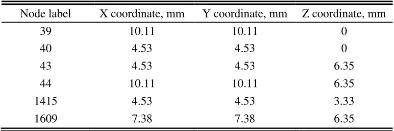
43→40, respectively. The global coordinates of all the nodes in Fig. 2.2 are shown in Table 2.3.
Table 2.3: Global coordinates of the nodes in Fig. 2.2
Node label X coordinate, mm Y coordinate, mm Z coordinate, mm
39 10.11 10.11 0
40 4.53 4.53 0
43 4.53 4.53 6.35
44 10.11 10.11 6.35
1415 4.53 4.53 3.33
1609 7.38 7.38 6.35
2.6 Boundary Conditions
Table 2.4 shows the necessary boundary conditions relevant to the boundaries as
described in Fig. 2.2 where is the displacement and is the rotation with 1, 2, and 3 as the
15
subscripts representing the X-, Y-, and Z-axes, respectively. The first boundary condition
indicates that the inner curved surface of the spur gear including the areas of the key slots does
not have any displacement along the X- or Y-directions i.e., along the radial direction. The only
direction to which the deformation is allowed is the Z-axis. This is because; after quenching, the
gear would have a tendency to shrink in all directions and if the inner curved surface of the
quarter gear including the key slot areas is not allowed to move radially, then the gear can shrink
only along the vertical direction.
Table 2.4: Boundary conditions for the quarter spur gear
Surfaces Degrees of freedom
UVWXABB′A′X′W′V′U′ U1=U2=UR3=0
BCC′B′ U2=UR1=UR3=0
UTT′U′ U1=UR2=UR3=0
CDEFGHIJKLMNOPQRSTUVWXAB U3=UR1=UR2=0
The second and the third boundary conditions indicate that the vertical planes
and ′ remain in the respective vertical planes while quenching. For plane ,
deformation is allowed along X- or Z-axis and rotation is constrained to occur only in the
XZ-plane (no rotation with respect to X- or Z-axis). For XZ-plane ′, deformation is allowed along
Y- or Z-axis and rotation is restricted to occur only in the YZ-plane (no rotation with respect to
Y- or Z-axis). These boundary conditions are set accordingly because both planes are the planes
of symmetry of the spur gear.
Finally, the fourth boundary condition describes that the bottom XY-plane remain in the
same plane and is not displaced. No rotation of this plane occurs with respect to the Z-axis. This
16
2.7 Mesh Generation
Figure 2.3: Mesh of the quarter gear with element size of 0.16 mm
The quarter gear is partitioned into eight segments to ensure a good, uniform mesh and to
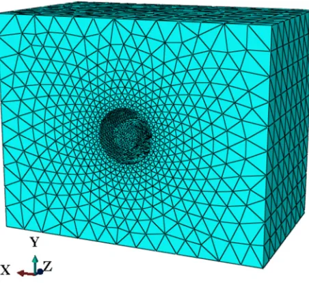
avoid deformation of mesh elements. Fig. 2.3 represents the meshed gear with the finest element
size of 0.16 mm. After meshing, the quarter gear has 156,640 elements and 169,412 nodes.
Structural meshing is preferred to avoid any distortion of the mesh elements. For fully coupled
analysis, C3D8RT (eight-node thermally coupled brick, tri-linear displacement and temperature,
reduced integration) elements are used. For sequentially coupled analysis, DC3D8 (eight-node
linear heat transfer brick) elements are used for heat transfer and C3D8R (eight-node, linear
17
3. Dynamic Quenching Analysis of a Steel Tube
3.1 Scope of Quenching of a Steel Tube
Steel tubes with various wall thicknesses are most commonly used as machine
components in a mechanism as connecting, rotating, or, rolling components, generator shafts,
pressure vessels, etc. They have to withstand high dynamic torsional and compressive stresses
and should have enhanced toughness and fatigue resistance for better performance and longer
life. Hence, steel tubes need to be quenched for obtaining improved properties. Since steel tubes
are the basic forms of many mechanical components, it is important to observe the transient
temperature distribution throughout the steel tube after quenching and the distribution of the
stress and deformation along radial and axial pathways of the tube. Therefore, in this Chapter, a
3-D FSI model is developed consisting of the solid steel tube and the liquid quenchant to
evaluate at first the thermal interaction between the tube and the quenchant. After that, the
thermal stress is calculated based on the previous thermal interaction. The time-varying
temperature distributions for three different nodes are investigated. Also, the residual stress and
deformation at a particular point and along the axial and radial directions of the tube after
quenching are studied. The cooling rates of all the three liquids are compared with each other and
the critical regions in the tube are identified after quenching.
3.2 Description of the Steel Tube
The steel tube has the inner and the outer radii of 1.2 mm and 2.5 mm, respectively, with
a height of 9.0 mm and is considered homogeneous. All the standard dimensions are chosen from
precision bushing catalog [34]. A relatively smaller tube is chosen to save computational time
18
3.3 Properties of the Steel Tube
Properties of the steel tube are given in Table 3.1 [18]. The tube is assumed to be made of
an elastic, perfectly plastic steel with a temperature dependent yield stress as mentioned in
Chapter 2 by Eqs. 1 and 2. All the properties of the steel tube are considered isotropic.
Table 3.1: Properties of the steel tube
3.4 Properties of the Liquid Quenchants
Three different liquid quenchants are used in this analysis namely water [35], 20% w/w
brine aqueous solution [36], and 10% w/w PG aqueous solution [37]. The properties of the liquid
quenchants at 25 °C are given in Table 3.2. The solution concentration unit w/w for both brine
and PG indicates the ratio of the mass of the solute to that of the solvent in a solution.
Table 3.2: Properties of the liquid quenchants at 25 °C
Property Water 20% w/w brine aqueous solution
10% w/w PG aqueous solution
Density, kg/m3 1000 1133 1004
Viscosity, Pa·s 0.891e–3 1.26e–3 1.2e–3
Thermal conductivity, W/m·K 0.61 0.494 0.565
Specific heat, J/kg·K 4200 3430 4200
Density, kg/m3 7830
Young’s modulus, Pa 206.8e9
Poisson’s ratio 0.3
Thermal conductivity, W/m·K 58.8
Specific heat, J/kg·K 600
19
3.5 The Fluid-Structure Interaction Model
The 3-D FSI model consists of the cylindrical steel tube as the solid FE model and the
rectangular liquid quenchant domain as the CFD model, for investigating the residual stress and
deformation in the tube by using the commercially available FE software, Abaqus 6.12 [33]. The
dynamic analysis is run in a transient mode by a sequentially coupled analysis. The sequentially
coupled analysis, as described in Chapter 2, consists of two steps; the pure transient heat transfer
analysis between the tube and the quenchant at first and then the thermal stress analysis of the
tube. In the first step, the heat transfer analysis is carried out by coupling the FE model with the
CFD model to generate the temperature-time history as an output until the tube reaches the sink
temperature. It is a multi-physics coupling such that the fluid flows over the tube and takes away
the heat to cool it. Once the temperature-time history in the heat transfer step is obtained, it is
used as an input in the second step where a static FE model is used to estimate the thermal stress
and deformation in the tube. The initial temperature of the tube and all the liquid quenchants are
850 °C [19] and 25 °C, respectively. The sink temperature for the tube is set as 25 °C.
3.5.1 General Mathematical Formulation for the CFD Model
T
he mathematical formulation for the CFD model predicts the primitive variables ofdensity, velocity, pressure, and temperature within the fluid domain which requires the solution
of the continuity, momentum (Navier-Stokes equations), and the energy equations. The general
mathematical formulation of the above conservation equations starting from vector form with
appropriate boundary conditions and initial conditions are discussed in the following sections.
Later, depending on our specific physical flow model, the corresponding boundary conditions
20
3.5.1.1 General Assumptions
1. The fluid flow is assumed to be incompressible.
2. The flow is laminar and viscous.
3. The working fluid behaves like a Newtonian fluid with stokes assumptions.
4. The physical properties of the fluids are assumed to be constant.
3.5.1.2 Conservation of Mass (Continuity Equation)
The general continuity equation in vector form for any fluid,
+ . = 0 (3.1)
where, indicates the velocity vector, is the density of the fluid, and represents
time.
From assumption 1, for incompressible flow,
= 0 (3.2)
Using the above relation in Eq. 3.1 and by assumption 4, the continuity equation becomes,
. = " (3.3)
From Eq. 3.3, the modified continuity equation can be written in scalar form,
#
$ +%& +'( = 0 (3.4)
where, #, %, and ' indicates the velocity components of the fluid in $, &, and ( directions,
respectively. Eq. 3.3 represents the most general form of the continuity equation for
21
3.5.1.3 Conservation of Momentum (Navier-Stokes Equations)
The general momentum equation in vector form for an incompressible flow with constant
properties (assumptions 1 and 4),
* + . + = −, + -∇/ + 0 (3.5)
where, , is the thermodynamic pressure, - is the dynamic viscosity of fluid, and 0is the
acceleration vector due to gravity.
The corresponding $, &, and ( momentum equations in scalar form are as follows:
*# + ##$ + %#& + '#(+ = −23−,$ + - 4
/#
$/ +
/#
&/+
/#
(/5 (3.6)
*% + #%$ + %%& + '%(+ = −27−,& + - 4
/%
$/ +
/%
&/+
/%
(/5 (3.7)
*' + #'$ + %'& + ''( + = −29−,( + - 4
/'
$/ +
/'
&/ +
/'
(/5 (3.8)
3.5.1.4 Conservation of Energy (Energy Equation)
The vector form of the energy equation for an incompressible flow the fluid domain can
be described as,
:;; = < ;,; − . = + Φ (3.9)
where,
: is the specific heat of the fluid at constant pressure
22 < is the volumetric thermal expansion coefficient = is the heat flux vector due to conduction, and
Φ is the dissipation function defined as,
Φ = @AB %A
$B (3.10)
where, @AB is the shear stress and CDE
C3F indicates the velocity gradient in the fluid domain.
If the velocity G becomes smaller and heat transfer remains important, the fluid kinetic
energy term containing G/ will eventually become much smaller than the enthalpy change
:Δ. Since both I:IJ and Φ are of order G/, we can neglect them and eventually Eq. 3.9
becomes,
:;; = −. = (3.11)
Neglecting radiative heat transfer, = can be calculated from Fourier’s law of heat
conduction,
= = −K (3.12)
where, K is the thermal conductivity of the fluid.
Substituting this value of =intoEq. 3.11, we get,
:;; = −. −K (3.13)
23
:4 + . 5 = K∇/ (3.14)
Eq. 3.14 can be expanded in scalar form in terms of the temperature gradients in $, &, and
( directions as,
:4 + # $ + %L& + 'L(5 = K 4
/
$/ +
/
&/ +
/
(/5 (3.15)
3.5.1.5 Boundary and Initial Conditions
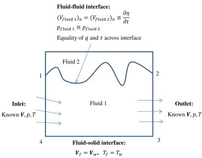
The boundary conditions for a viscous, heat conducting flow involve three most common
type of boundaries described in Fig. 3.1,
1. The fluid-solid interface
2. The fluid-fluid interface
3. The inlet or exit section of the fluid domain
1. The fluid-solid interface: At the fluid-solid interface, there must be no slip of fluid
due to viscosity effect. So, the no slip boundary conditions are,
= M or = N (3.16)
where, the subscripts L, O, and ' stands for fluid, solid, and wall, respectively.
When, the fluid conducts heat from the wall, then, either there will be no temperature jump
(when the wall temperature is known or can be found from other relationships),
= M or = N (3.17)
24
KP = Q (3.18)
where, P indicates the direction normal to the fluid surface adjacent to the wall.
Figure 3.1: Typical boundary conditions in a viscous heat-conducting fluid flow analysis
2. The fluid-fluid interface: At the interface between two fluids, there must be
kinematic equivalence, i.e., there must be equality of the normal velocity across the fluid-fluid
interface so that no holes appear between them, which is also known as the kinematic boundary
condition. If we denote the fluid 1 and fluid 2 interface 1-2 in Fig. 3.1 by R, then the boundary
condition at the interface 1-2 would be,
(GSTAU V)W = (GSTAU /)W ≅ R (3.19)
1
4 3
2
Inlet:
Known , ,,
Outlet:
Known , ,,
(GSTAU V)W = (GSTAU /)W ≅ R
,STAU V ≅ ,STAU /
Fluid-fluidinterface:
Equality of Q and @ across interface
Fluid-solid interface:
= N, = N
25
There must be mechanical equilibrium across the interface. The viscous shear stresses
must balance:
@STAU VAWJYZ[\Y = @STAU /AWJYZ[\Y (3.20)
Neglecting the viscous normal stresses, the pressure at the interface except for surface
tension effects (negligible in most cases) must be balanced as,
,STAU V ≈ ,STAU / (3.21)
Finally the heat transfer must be same on both sides of the interface, since no heat can be
stored in the infinitesimally thin interface and neglecting radiation which is equivalent to
QSTAU VW = QSTAU /W (3.22)
3. The inlet or exit section: At any inlet or outlet section of the flow, the complete
distribution of the velocity, pressure, and temperature must be known every point on the
boundary which sets the boundary conditions as; known G, ,, and at inlet and exit.
If the flow is unsteady, there must be an initial condition or initial spatial distribution
known for the primitive variables. Hence, for the most general case, the initial condition is
written as; known G, ,, and at = 0, where G, ,, and are different functions of $, &, and (.
3.5.2 Physical Domain
Figures 3.2 and 3.3 show the computational fluid domain for the liquid quenchant and the
steel tube, respectively. The point of origin for both the fluid and the solid domain is the
intersection of the X-, Y-, and Z-axes which lies in the same XY-plane common for both
26
the X-direction, the width of 20 mm in the Y-direction, and the height of 15 mm in the Z
-direction. The solid domain in Fig. 3.3 has the same dimensions as described before for the steel
tube in the property section. The surface of the tube in the XY-plane is will be noted asthe
bottom surface of the tube.
Figure 3.2: Computational domain for the liquid quenchant
Figure 3.3: Computational domain for the steel tube
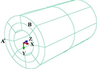
Figure 3.4 describes the longitudinal cross-section of the steel tube about the YZ-plane
where an axial path AB from node 52 to node 25 and a radial path CD from node 68 to node 27,
are created to see the distribution of the stress and deformation along the normalized distance.
The normalized distance is a dimensionless distance defined as the ratio of any distance from the
27
and K are randomly chosen in the tube. Node J is located on the top surface of the tube in the
upstream direction of flow on the periphery of a circle having a radius of 1.85 mm along
negative X-axis. Node K is located in the longitudinal cross-section FGHI of the tube near the
vicinity of the bottom surface. Node E is the intersection point as well as the midpoint of both
paths AB and CD. Table 3.3 enumerates the coordinates of all the nodes described in Fig. 3.4.
Figure 3.4: Half of the tube with locations of paths (AB and CD) and nodes (2, 24, 25, 27, 52, 68, and 2471) of analysis
Table 3.3: Global coordinates of the nodes in Fig. 3.4
Node label
X-coordinate,
mm
Y-coordinate,
mm
Z-coordinate,
mm
2 -1.85 0 9
24 0 -1.85 4.5
25 0 -1.85 9
27 0 -2.5 4.5
52 0 -1.85 0
68 0 -1.2 4.5
28 3.5.3 Interaction
The interaction surface is the common, shared surface between the tube and the
quenchant through which heat transfer occurs. The whole surface area of the tube except the
bottom surface is the interaction surface also known as fluid-structure co-simulation boundary.
The interaction surface for the tube can be visualized easily from Fig. 3.2 which is the union of
the top surface J, the outer surface K, and the inner surface L of the tube inside the fluid domain.
3.5.4 Boundary and Initial Conditions
3.5.4.1 For CFD Model
Table 3.4: Boundary conditions for fluid domain
Name Surfaces
Boundary conditions
Velocity, m/s
# % ' Pressure, Pa Temperature, ºC
In-flow ABDC 1 0 0 - -
Top-flow ABFE 1 0 0 - -
Side-flow BFGD 1 0 0 - -
Side-flow AEHC 1 0 0 - -
Out-flow EFGH - - - 0 -
No-slip CDGH+I+J+K+L 0 0 0 - -
No-temperature jump CDGH+I+J+K+L 0 0 0 - = M^SAUMTZ[\Y
The boundary conditions for the CFD model (the fluid domain) are shown in Table 3.4
with reference to Fig 3.2. For the fluid domain, the boundary conditions are specified in terms of
velocity, pressure, or temperature. As mentioned in the mathematical formulation;#, %, and '
indicate the velocity components along X-, Y-, and Z-directions (upper case notations according
29
are considered the same as that for the in-flow. This is because; the fluid domain is small enough
to justify the consideration of parallel flow. It is a reasonable assumption to set zero velocity in
Y- and Z-directions. The no-slip boundary condition contains surface CDGH and surface I in
Fig. 3.2 including the interaction surface. The no-temperature jump boundary condition indicates
that at the hot outer and inner surfaces of the steel tube, the adjacent fluid layers in touch must
have the same temperature of the corresponding surfaces.
The heat from the hot solid surface of the steel tube to the liquid is transferred in two
steps. At first, the heat will transfer from the hot tube surface to the touching adjacent but very
thin stagnant layer of liquid mainly by conduction through the thickness of the layer and also by
convection which is negligible. In the next step, the heat from the thin liquid layer will negligibly
be conducted to the surrounding fluid buy significantly by convection. Mathematically, we can
express this by,
(_\^WUT\JA^W+ _\^WDY\JA^W)J`AW S[7YZ = (_\^WUT\JA^W+ _\^WDY\JA^W)MTZZ^TWUAWa STAU
(_\^WUT\JA^W)J`AW S[7YZ≅ (_\^WDY\JA^W)MTZZ^TWUAWa STAU
− *Kb3cc$ +Kb7cc& + Kb9cc(+ ≅ ℎbS[7YZ− ZYYMJZY[e (3.23)
where,
_ is the heat transferred either by conduction or convection
b3, b7, and b9 indicate the heat conduction areas in the thin liquid layer normal to the
$, &, and ( directions, respectively
30
bS[7YZ is the outer area of the thin fluid layer separating the bulk fluid from the tube wall
Uf
U3
,
cc&,
and UfU9 indicate the temperature gradients in the thin liquid layer in $, &, and (direction respectively and the temperature derivative is defined as,
c
cP = limjW→l
WmjW− W
ΔP = limjW→l
M^SAUMTZ[\Y−
ΔP
where, P indicates either $, &, or ( direction.
Since we are not considering a steady flow analysis, the initial conditions must be defined
at the start of our analysis for the CFD model. The initial conditions are stated below:
1. Initial condition for velocity: The free stream velocity of fluid applied at the left
boundary of the fluid domain in Fig. 3.2 represents the initial velocity condition as; # = 1 n/O,
% = 0, and ( = 0 at = 0.
2. Initial condition for temperature: It is the temperature of the fluid in the free stream
location applied at the left boundary of the CFD model in Fig. 3.2 and is prescribed as =
25 °C at = 0.
3.5.4.2 For Solid Model
For the solid domain, the boundary conditions are specified in terms of the displacement
and the rotation with reference to Fig. 3.3. In Table 3.5, O and p indicate the displacement and the
rotation of the tube, respectively, with the corresponding subscripts. For the solid domain in Fig.
3.3, surface B is the whole bottom surface of the tube which always remains in XY-plane during
quenching for which O9 is zero. The fixed point A is located on the bottom surface of the tube in
31
displacements and rotations are zero on that point. The initial condition for the solid tube in
terms of temperature is set as; N`^SYJTqY = M^SAUMTZ[\Y =850 °C at = 0.
Table 3.5: Boundary conditions for solid domain
Name
Surface or point
Boundary conditions
Displacement, m Rotation, degrees
O3 O7 O9 p3 p7 p9
Bottom surface B - - 0 - - -
Fixed point A 0 0 0 0 0 0
3.5.5 Mesh Generation
3.5.5.1 For CFD Model
Figure 3.5: The fluid domain after meshing
Figure 3.5 shows the meshed fluid domain with the finest element size of 2 mm. A high
density mesh is created near the outer and the inner surface of the cavity within the fluid domain
32
cavity. The rectangular fluid domain in the CFD model is meshed by FC3D4 (four-node, linear,
fluid-tetrahedron), 3-D stress elements.
3.5.5.2 For Solid Model
Figure 3.6: The steel tube after meshing
Figure 3.4 represents the meshed FE model of the steel tube with the finest element size
of 0.2 mm. For more accuracy, structured meshing is considered. The tube is symmetrically
partitioned by eight axial planes and by one radial plane through the center of the tube axis. After
meshing, the tube has 15,456 elements and 18,424 nodes which are kept same for both heat
transfer and thermal stress analyses. In this sequentially coupled analysis, DC3D8 (eight-node
linear heat transfer brick) elements are used for the heat transfer step and after that, C3D8R
(eight-node, linear brick, reduced integration) elements are used to calculate the 3-D stress. The
solid FE model developed in Abaqus/Standard and the CFD model developed in Abaqus/CFD
33
4. Results and Discussions
4
.1 Static Quenching Analysis of a Spur Gear
4.1.1 Model Validation
For validating the FE model, the residual stress computed by Landau et al. [18] for an
infinite plate with one-dimensional (1-D) heat transfer is compared with that of the developed FE
model. Landau et al. [18] showed the residual stress distribution after quenching of an infinite
steel plate of thickness 36 inch only in the thickness direction. An axisymmetric analysis from
center of the plate up to thickness of 18 inch was carried out. The boundary conditions of the
axisymmetric model involved no movements of the X- and Y-axes, in vertical and horizontal
directions, respectively. The FE model computes the 1-D residual stress as reported in Ref. [18]
by both fully and sequentially coupled analyses. The maximum variation of the stress computed
by two models (Ref. [18] and developed FE model) is 8%. As the FE model for 1-D quenching
workes well, the current 3-D model of the gear is investigated for further analysis.
In this analysis of the quarter gear in Chapter 2, the estimates are in an excellent
agreement with both fully and sequentially coupled analysis for the finest mesh size of 0.16 mm.
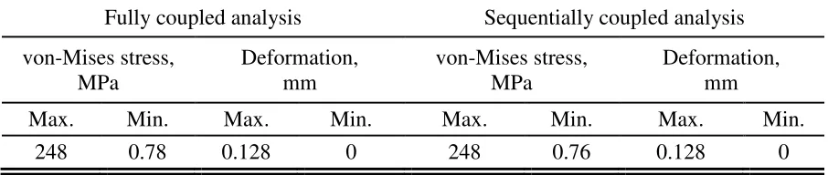
A comparison of the results from both methods is shown in Table 6.
Table 4.1: Comparison of fully coupled and sequentially coupled analysis
Fully coupled analysis Sequentially coupled analysis
von-Mises stress, MPa
Deformation, mm
von-Mises stress, MPa
Deformation, mm
Max. Min. Max. Min. Max. Min. Max. Min.
34
4.1.2 Convergence Study and the Cooling Curve
Figure 4.1 shows the variation of stresses at different nodes with degrees of freedom
(DOF) for different meshes. 14 different mesh elements of size 2.0, 1.8, 1.5, 1.2, 1.0, 0.8, 0.5,
0.4, 0.3, 0.25, 0.22, 0.2, 0.18, and 0.16 mm are used for the simulation until the convergence or
mesh independence condition is obtained. As the DOFs increase, stresses fluctuate initially and
after that become flattened indicating that the solution has already become mesh independent.
The mesh independence study is done for three different nodes as shown in Fig. 4.1.
Figure 4.1: Variations of the von-Mises stresses at different nodes with degrees of freedom
Figure 4.2 gives the temperature-time history for five nodes located in surface ABCD, the
middle vertical plane in the quarter gear in Fig. 2.2. Nodes 39, 44, and 1609 are on the boundary
while nodes 14983 and 15979 are internal ones. The temperature of each node decreases with
time in an exponential way as the gear cools from 850 °C to 25 °C. The cooling curves for nodes
14983 (X=5.43712 mm, Y=5.43789 mm, and Z=1.11125 mm) and 15979 (X=6.80506 mm,
Y=6.80603 mm, and Z=4.445 mm) are the top ones indicating lower cooling rates compared to
von
-M
is
es
s
tr
es
s, M
P
35
those of nodes 39, 44, and 1609 as they did not come directly to the exposure of the cooling
environment. The time-varying temperature distribution for each node follows similar trend up to
15 s and are merged after that. It is clear from the cooling curve that the cooling rate decreases as
the temperature difference between the gear and the surrounding decreases. The slopes of the
cooling curves indicate respective cooling rates almost zero after 15 s for all of the nodes.
Figure 4.2: Variations of the nodal temperatures with time
4.1.3 Stress and Deformation Analysis
Figure 4.3: Distribution of the von-Mises stress in the quarter gear von-Mises Stress,
MPa
.
.
.
.
.
44
1609
15979
14983 39
D C
B
36
From Fig. 4.3, the highest stress developed in the gear is 248 MPa that covers the region
from the inner bore edge up to the tooth root and reduces from the tooth root to the tooth tip of
the gear radially inwards. The stress also varies through the tooth along the gear thickness. From
Fig. 4.4, the deformation varies from the bottom plane to the top plane of the gear and increases
from the inner bore edge to the tooth tip with a peak value of 0.128 mm.
Figure 4.4: Distribution of the deformation in the quarter gear
4.1.4 Time-varying Nodal Stress and Deformation
The behavior of the time-varying stresses at nodes 39, 1415, and 1609 are plotted in Fig.
4.5 which depicts that after around 7 s, all the curves get flattened, although they have some
initial stress fluctuations. Nodes 39 and 1415 have the leveled stress of 84 MPa and 284 MPa,
respectively. The stress for node 1609 is 181.4 MPa for most of the time. Node 1415 has higher
stress than that of node 1609, as the former is located on a curved surface. The behavior of the
time-varying deformations at nodes 39, 1415, and 1609 are visible in Fig. 4.6 where all the
curves show a sharp increase of deformation within 5 s. Compared to Fig. 4.5, node 39 has no
fluctuation in deformation as seen from Fig. 4.6. Also, from Fig. 4.6, the deformations of nodes
39 and 1609 are very close unlike respective stresses given by Fig. 4.5.
37
Figure 4.5: Variations of the von-Mises stresses at different nodes with time
Figure 4.6: Variations of the deformations at different nodes with time
4.1.5 Path-wise Stress and Deformation
The variation of the von-Mises stress with normalized distance along the pathway from
node 39 to node 40 is given in Fig. 4.7 where the normalized distance is calculated by dividing
the distance of any node from node 39 by the total linear distance between node 39 and node 40.
von
-M
is
es
s
tr
es
s,
M
P
38
Fig. 4.7 gives a fluctuating pattern of stress along the path from node 39 to node 40 (pathway
39→40). As node 39 is more constrained than the top nodes, it shows the highest stress of 84
MPa among all the nodes in the pathway 39→44 and starts decreasing after that until it reaches
node 44 at a normalized distance of 0.3 with 2 MPa stress. For pathway 44→43, the stress level
increases, then decreases, and again increases ending up to 248 MPa at normalized distance 0.53
and continues the trend up to node 40. The overall stress fluctuation is due to the unequal
movement of the inner nodes not very free to move compared to the outer ones.
Figure 4.7: Variation of the von-Mises stress along the path 39→40
Comparing Figs. 4(b) and 5(b), a trend of decreasing stress in Fig. 4(a) is counter parted
by increasing deformation in Fig. 5(b) within node path 39→44. The opposite behavior is seen
for node path 44→43. The highest stress developed in the gear is the plastic yield stress limit of
the gear material; consequently, a proportional stress-strain relationship within the elastic limit
does not work. For node path 39→44, the upper nodes are freer to move compared to node 39
and they experience more deformation. Due to the constraint, the bottommost node 39 shows the
von
-M
is
es
s
tr
es
s,
M
P
a
0
0.2
0.4
0.6
0.8
1
0
50
100
150
200
250
39
Figure 4.8: Variation of the deformation along the path 39→40
least deformation but higher stress up to node 44 when considered the pathway 39→44. For
pathway 44→43, the nodes at the outer edge of the quarter gear have more freedom to move then
the inner ones (partially constrained), which is the cause of the fall of deformation to a value of
0.076 mm at node 43 (normalized distance 0.69) in Fig. 4.8. For pathway 43→40, the
deformation continuously decreases and becomes zero at the mid-plane since the corresponding
boundary conditions restrict the X-, Y-, and Z-movements accordingly. When comparing Figs.
4.5 and 4.6, the stress at node 39 is the least among all the three nodes while the deformation of
node 39 is the highest. This is because; node 39 is located on the outermost edge of the quarter
gear. As there is no constraint for node 39 to move freely in the radial direction, the stress at node
39 would be the minimum and the corresponding deformation of node 39 would be the
maximum. From Fig. 4.5, node 1415 has higher stress than that of node 1609 because node 1415
has only one DOF (vertical) while node 1609 has more than one DOFs. The corresponding
deformations of the nodes 1415 and 1609 are reflected in Fig. 4.6, where node 1609 shows
higher deformation than that of node 1415.
0
0.2
0.4
0.6
0.8
1
0
0.05
0.1
0.15
0.2
Normalized distance from node 39 to node 40
D
ef
o
rm
at
io
n
,
m
40
4.2 Dynamic Quenching Analysis of a Steel Tube
4.2.1 Model Validation
The model is validated by the experimental results as described in Chapter 4 in section 4.1.1.
4.2.2 Convergence Study and the Cooling Curve
Figure 4.9: Variations of the temperatures of node 24 with degrees of freedom
The variations of the temperature of node 24 (point E of Fig. 3.4) versus the degrees of
freedom (DOF) are depicted in Fig. 4.9 for two different time steps; 0.4 s and 2 s. The reason for
choosing 0.4 s is because; the major fluctuation of temperature occurs within a very short period
of time after the quenching starts. From Fig. 4.9, as the DOF increases, the temperature becomes
flattened after showing some initial changes indicating that the solution is already converged and
has become mesh independent. Mesh independence studies are done for both the solid FE and
CFD models. At first, the CFD model is made mesh independent with the finest element size of 2
mm. Later the FE model is made so with the finest element size of 0.2 mm based on the former.
0
0.5
1
1.5
2
x 10
4100
200
300
400
500
600
700
800
Degrees of freedom
T
em
p
er
at
u
re
,
°C
41
Figure 4.10 gives the temperature-time history for nodes 2, 24, and 2471 (points J, E, and
K, respectively, of Fig. 3.3) quenched by water, whose coordinates are given in Table 3.3. As
seen for static analysis in Fig. 4.2, the temperature of each node decreases exponentially with
time as the tube cools from 850 °C to 25 °C. All the cooling curves follow the similar trend up to
4 s and are merged after that. It is reasonable to assume that the cooling curves for these three
nodes would be of similar shapes for other quenchants but with different cooling rates.
Figure 4.10: Variations of the temperatures of nodes 2, 24, and 2471 with time for water
To compare the cooling capacities for different quenchants, Fig. 4.11 shows the
time-varying temperatures of node 24 by water, brine, and PG. The time scale chosen here is
logarithmic unlike linear to observe the actual characteristics of the cooling curves. It shows the
portion of the cooling curve where the rate of change of temperature (cooling rate or slope of the
cooling curve) is very high. Therefore, compared to Fig. 4.10, Fig. 4.11 reveals that rapid cooling
of the tube occurs from 0.1 s to 1 s. The time required to cool the tube to the sink temperature is
8 s, 9.5 s, and 8.6 s for water, brine, and PG, respectively. Starting from the same time, the
0 2 4 6 8
0 200 400 600 800 1000
Time, s
T
em
p
er
at
u
re
,
°
C
42
Figure 4.11: Variations of the temperatures of node 24 with time for different quenchants
cooling curve for brine is always above that of water indicating less cooling capacity than water
while PG maintains a cooling capacity somewhere in between that of water and brine. The
concentration of the aqueous solution as a quenchant affects the cooling rate. The properties of
the aqueous solution become closer to water as the concentration of the solution becomes lower.
4.2.3 Stress and Deformation Analysis
Figures 4.12 through 4.15 describe the deformed contour of the steel tube for water
quenching in terms of the von-Mises stress and the deformation. Similar characteristics of the
deformed contour of the tube are found for brine and PG also, with only some variations in the
magnitudes of the stress and deformation. From Figs. 4.12(a) and 4.12(b), the highest von-Mises
stress generated in the tube is 45.95 kPa, which occurs in the lower-half of the outer surface and
the mid-internal surface of the tube in the downstream direction of flow. The magnitude of the
highest stress is below the yield stress limit of the steel tube. Therefore, it is reasonable to
assume that the steel retains its elastic strain-strain behavior throughout the analysis.
10-3 10-2 10-1 100 101
0 200 400 600 800 1000
Time, s
T
em
p
er
at
u
re
,
°C