Motion Dynamics of Dropped Cylindrical Objects

University of New Orleans University of New Orleans

ScholarWorks@UNO

ScholarWorks@UNO

University of New Orleans Theses and

Dissertations Dissertations and Theses

Spring 5-19-2017

Motion Dynamics of Dropped Cylindrical Objects

Motion Dynamics of Dropped Cylindrical Objects

Gong Xiang

University of New Orleans, [email protected]

Follow this and additional works at: https://scholarworks.uno.edu/td

Part of the Ocean Engineering Commons, and the Risk Analysis Commons

Recommended Citation Recommended Citation

Xiang, Gong, "Motion Dynamics of Dropped Cylindrical Objects" (2017). University of New Orleans Theses and Dissertations. 2340.

https://scholarworks.uno.edu/td/2340

Motion Dynamics of Dropped Cylindrical Objects

A Dissertation

Submitted to the Graduate Faculty of the University of New Orleans

in partial fulfillment of the requirements for the degree of

Doctor of Philosophy

in Engineering and Applied Science

Naval Architecture and Marine Engineering

by

Gong Xiang

B.S. Huazhong University of Science and Technology 2011 M.E. Stevens Institute of Technology 2013

Copyright 2017, Gong Xiang

Acknowledgement

I would like to express the deepest appreciation to my committee chair Professor Lothar Birk and co-chair Professor Xiaochuan Yu. They continually and convincingly conveyed a spirit of adventure in regard to research and an excitement in regard to teaching. Without their guidance and persistent help this dissertation would not have been possible.

I would like to thank my committee member, Professor Brandon Taravella who recruited me into UNO’s PhD program and gave me clear guidance on finishing all the official requirements for the degree.

In addition, thank Professor Linxiong Li and Professor Uttam K Chakravarty for serving on my committee.

Contents

Contents v

List of Figures vii

List of Tables xi

Symbols xii

Abbreviations xiv

Abstract xv

1 Introduction 1

2 Literature Review 4

3 2D theory of dropped cylinderical object 10

3.1 2D Equations of motion for rigid body . . . 10

3.1.1 Hydrodynamic force and moment in potential theory . . . 12

3.1.2 Viscosity . . . 13

3.1.3 Transformation of coordinate system . . . 14

3.2 Simulated trajectories of dropped cylindrical objects using 2D theory . . . 15

4 3D theory of dropped cylinderical object 19 4.1 3D Equations of motion of rigid body . . . 19

4.1.1 Rigid body kinematics . . . 19

4.1.2 Rigid body dynamics . . . 20

4.1.3 Transformation of coordinate system . . . 23

4.1.4 Equations of motion for dropped cylindrical object . . . 26

4.1.5 Hydrodynamic force and moment in potential theory . . . 29

4.1.6 Viscosity . . . 29

4.1.7 Lift theory . . . 30

4.1.8 Transformation of coordinate system . . . 32

4.2 Comparison of dropped cylindrical objects using 2D theory and 3D theory . . . . 33

4.3 Study of factors influencing trajectories . . . 34

4.4.1 Rigid body kinematics . . . 54

4.4.2 Rigid body dynamics . . . 54

4.4.3 Equations of motion for dropped objects with nonzero LCG . . . 56

4.5 Dropped objects under current . . . 67

4.5.1 Uniform current . . . 68

5 Statistical study on landing points of dropped cylindrical object falling through air-water columns 73 5.1 Monte Carlo method . . . 73

5.2 Description of random variables . . . 76

5.2.1 Fundamentals of distribution selection . . . 76

5.2.2 Sensitivity analysis . . . 77

5.3 Sampling process . . . 78

5.4 Results of estimated landing point distribution under no current . . . 81

5.4.1 DNV simplified method . . . 81

5.4.2 Monte Carlo method: sensitivity analysis of mean value forZ˙0 . . . 82

5.4.3 Monte Carlo method: sensitivity analysis of value of standard deviation forθ0andΩ2 . . . 84

5.4.4 Simulated landing point distributions under uniform current . . . 86

5.5 Statistical analysis of simulated landing point distribution . . . 94

5.5.1 Mean, Median, Maximum (Max), Minimum (Min), Standard Deviation (SD) and confidence interval of excursion . . . 94

5.5.2 Risk free zone . . . 95

6 Conclusions 100 6.1 Conclusions . . . 100

6.2 Future work . . . 102

Bibliography 104

List of Figures

2.1 Sketches of observed trajectories (Aanesland, 1987) . . . 5 2.2 Coordinate system for equation of motions in three dimensions (Kim et al. 2002) 6 2.3 Experimental equipments: (A) drop angle device, (B) cylinder injector, (C)

in-frared light sensor, (D) output to universal counter, and (E) cylinders.(Chu et al.2005; 2006) . . . 7 2.4 Top view of the cylinder drop experiment.(Chu et al. .2005; 2006) . . . 8

3.1 Coordinate system for equation of motions in two dimensions . . . 11 3.2 Simulated trajectory and experimental envelope at drop angle45o,Cdz = 1.0, by

Aanesland (1987) . . . 16 3.3 Comparison of repeated simulated trajectory at drop angle45o,Cdz = 1.0, with

experimental envelope by Aanesland (1987) . . . 16 3.4 Simulated trajectory and experimental envelope at drop angle 30o, Xt=0.4, by

Aanesland (1987) . . . 17 3.5 Comparison of repeated simulated trajectory at drop angle30o, Xt=0.4, with

ex-perimental envelope by Aanesland (1987) . . . 17 3.6 Simulated trajectory and experimental envelope at drop angle 60o_{, Xt=0.4, by}

Aanesland (1987) . . . 18 3.7 Comparison of repeated simulated trajectory at drop angle60o, Xt=0.4, with

ex-perimental envelope by Aanesland (1987) . . . 18

4.1 Coordinate system for equation of motions in three dimensions . . . 27 4.2 Lift force of a rotating cylinder as a function of speed ratio . . . 32 4.3 Comparison of simulated trajectories of dropped cylinder at drop angle45owith

variance of Xt using 2D theory in Aanesland (1987) and new 3D theory with

Vroll= 0. . . 34

4.4 Simulated X-Z plane trajectories with variance ofCdz at drop angle30o, Xt=0.4,

Vroll=0.05rad/s,Cdy=1.0 . . . 35

4.5 Simulated X-Z plane trajectories with variance ofCdz at drop angle45o, Xt=0.4,

Vroll=0.05rad/s,Cdy=1.0 . . . 36

4.6 Simulated X-Z plane trajectories with variance ofCdz at drop angle60o, Xt=0.5,

Vroll=0.05rad/s,Cdy=1.0 . . . 36

4.7 Simulated X-Z plane trajectories with variance ofCdy at drop angle30o, Xt=0.4,

Vroll=0.05rad/s,Cdz=1.0 . . . 37

4.8 Simulated X-Z plane trajectories with variance ofCdy at drop angle45o, Xt=0.4,

Vroll=0.05rad/s,Cdz=1.0 . . . 38

4.9 Simulated X-Z plane trajectories with variance ofCdyat drop angle60o, Xt=0.4,Vroll=0.05rad/s,

4.10 Simulated Y-Z plane trajectories with variance ofCdyat drop angle30o, Xt=0.4,

Vroll=0.05rad/s,Cdz=1.0 . . . 39

4.11 Simulated Y-Z plane trajectories with variance ofCdyat drop angle45o, Xt=0.4, Vroll=0.05rad/s,Cdz=1.0 . . . 40

4.12 Simulated Y-Z plane trajectories with variance ofCdyat drop angle60o, Xt=0.5, Vroll=0.05rad/s,Cdz=1.0 . . . 40

4.13 Simulated X-Z plane trajectories with variance ofVrollat drop angle30o, Xt=0.4,Cdy=1.0, Cdz=1.0 . . . 41

4.14 Simulated X-Z plane trajectories with variance ofVrollat drop angle45o, Xt=0.4,Cdy=1.0, Cdz=1.0 . . . 42

4.15 Simulated X-Z plane trajectories with variance ofVrollat drop angle60o, Xt=0.4,Cdy=1.0, Cdz=1.0 . . . 42

4.16 Simulated 3D trajectories with variance ofVrollat drop angle30o, Xt=0.4,Cdy=1.0, Cdz=1.0 andVroll=0.1 rad/s . . . 43

4.17 Simulated time domain translational motions (a) in X-direction (b) in Y-direction (c) in Z-direction (from top to bottom) . . . 44

4.18 Simulated X-Z plane trajectories with drop angle from0oto90o,Cdy=1.0,Cdz=1.0, Vroll=0.01 rad/s . . . 45

4.19 Simulated Y-Z plane trajectories with drop angle from0oto90o,Cdy=1.0,Cdz=1.0, Vroll=0.01 rad/s . . . 46

4.20 Excursion distribution at 5m water depth with drop angles from0o_to90o_,C dy= 1.0, Cdz = 1.0, Vroll = 0.01rad/s, global view . . . 47

4.21 Excursion distribution at 5m water depth with drop angles from0oto90o,Cdy= 1.0, Cdz = 1.0, Vroll = 0.01rad/s, local view(Y axis scale enlarged) . . . 48

4.22 3D Simulated orientation and trajectory for drop angle30o . . . 49

4.23 The velocity time series of surge . . . 49

4.24 The velocity time series of sway . . . 50

4.25 The velocity time series of heave . . . 50

4.26 The velocity time series of roll . . . 51

4.27 The velocity time series of pitch . . . 51

4.28 The velocity time series of yaw . . . 52

4.29 Time series of the Euler angle in roll direction . . . 52

4.30 Time series of the Euler angle in pitch direction . . . 53

4.31 Time series of the Euler angle in yaw direction . . . 53

4.32 Set up of the cylinders dropped into water . . . 56

4.33 Simulated trajectory with variance of Xt atθ0=30o . . . 59

4.34 Simulated trajectory with variance of Xt atθ0=45o . . . 60

4.35 Simulated trajectory with variance of Xt atθ0=60o . . . 60

4.36 Trajectory of cylinder#2 with drop angle45o: (a) Chu et al. (2005) . . . 62

4.37 Trajectory of cylinder#2 with drop angle45o: (b) DROBS . . . 63

4.38 Trajectory of cylinder#3 with drop angle45o: (a) Chu et al. (2005) . . . 64

4.39 Trajectory of cylinder#3 with drop angle45o: (b) DROBS . . . 65

4.40 Trajectory of cylinder#2 with varying LCG, drop angle45o _{. . . 66}

4.41 Coordinate system for equation of motions in three dimensions . . . 67

5.2 Schematic showing the principal of stochastic uncertainty propagation (Monte

Carlo Simulation Basics2004) . . . 76

5.3 Histogram of sampling distribution ofθ0 . . . 79

5.4 PDF of sampling distribution and true distribution ofθ0. . . 79

5.5 Histogram of sampling distribution ofΩ0 . . . 80

5.6 PDF of sampling distribution and true distribution ofΩ0 . . . 80

5.7 Landing point distribution drop angle60o_withZ˙_{0 ∼N(0.90Vmax,0.1}2_{) . . . 82}

5.8 Landing point distribution drop angle60owithZ˙0 ∼N(0.75Vmax,0.12) . . . 83

5.9 Landing point distribution drop angle60owithZ˙0 ∼N(0.50Vmax,0.12) . . . 83

5.10 Landing point distribution drop angle60owithθ0∼N(1.05,(0.6 + 0.01)2) . . . . 85

5.11 Landing point distribution drop angle60owithθ0∼N(1.05,(0.6−0.01)2) . . . . 85

5.12 Landing point distribution drop angle60owithΩ0∼N(0,(3 + 0.1)2) . . . 86

5.13 Landing point distribution drop angle60o_withΩ 0∼N(0,(3−0.1)2) . . . 86

5.14 Drop angle0owith Z˙0 ∼ N(0.5Vmax,0.12), θ0 ∼ N(0,0.62),Ω20 ∼ N(0,32): (a) Landing point distribution . . . 87

5.15 Drop angle0o with Z˙0 ∼ N(0.5Vmax,0.12), θ0 ∼ N(0,0.62),Ω20 ∼ N(0,32): (b) Histogram of excursion . . . 88

5.16 Drop angle15o_withZ˙_{0 ∼N(0.5Vmax,0.1}2_{), θ} 0 ∼N(0,0.62),Ω20 ∼N(0,32): (a) Landing point distribution . . . 88

5.17 Drop angle15owithZ˙0 ∼N(0.5Vmax,0.12), θ0 ∼ N(0,0.62),Ω20 ∼N(0,32): (b) Histogram of excursion . . . 89

5.18 Drop angle30owithZ˙0 ∼N(0.5Vmax,0.12), θ0 ∼N(0,0.62),Ω20 ∼N(0,32): (a) Landing point distribution . . . 89

5.19 Drop angle30owithZ˙0 ∼N(0.5Vmax,0.12), θ0 ∼ N(0,0.62),Ω20 ∼N(0,32): (b) Histogram of excursion . . . 90

5.20 Drop angle45owithZ˙0 ∼N(0.5Vmax,0.12), θ0 ∼N(0,0.62),Ω20 ∼N(0,32): (a) Landing point distribution . . . 90

5.21 Drop angle45owithZ˙0 ∼N(0.5Vmax,0.12), θ0 ∼ N(0,0.62),Ω20 ∼N(0,32): (b) Histogram of excursion . . . 91

5.22 Drop angle60owithZ˙0 ∼N(0.5Vmax,0.12), θ0 ∼N(0,0.62),Ω20 ∼N(0,32): (a) Landing point distribution . . . 91

5.23 Drop angle60o_withZ˙_{0 ∼N(0.5Vmax,0.1}2_{), θ} 0 ∼ N(0,0.62),Ω20 ∼N(0,32): (b) Histogram of excursion . . . 92

5.24 Drop angle75owithZ˙0 ∼N(0.5Vmax,0.12), θ0 ∼N(0,0.62),Ω20 ∼N(0,32): (a) Landing point distribution . . . 92

5.25 Drop angle75owithZ˙0 ∼N(0.5Vmax,0.12), θ0 ∼ N(0,0.62),Ω20 ∼N(0,32): (b) Histogram of excursion . . . 93

5.26 Drop angle90owithZ˙0 ∼N(0.5Vmax,0.12), θ0 ∼N(0,0.62),Ω20 ∼N(0,32): (a) Landing point distribution . . . 93

5.27 Drop angle90owithZ˙0 ∼N(0.5Vmax,0.12), θ0 ∼ N(0,0.62),Ω20 ∼N(0,32): (b) Histogram of excursion . . . 94

5.28 Histogram of excursion of landing points, R withZ˙0 ∼N(0.50Vmax,0.12), θ0 ∼ N(0,0.62),Ω20∼N(0,32) . . . 95

5.29 PDF of excursion of landing points, R withZ˙0 ∼N(0.50Vmax,0.12), θ0∼N(0,0.62),Ω20∼ N(0,32) . . . 96

5.30 CDF of excursion of landing points, R withZ˙0 ∼N(0.50Vmax,0.12), θ0 ∼N(0,0.62),Ω20∼ N(0,32) . . . 96

5.32 Impact energy distribution for drop angle at60o: (a) without current . . . 98 5.33 Impact energy distribution for drop angle at60o: (b) current with speed 0.5m/s

List of Tables

1.1 Frequencies for dropped objects into the sea (DNV, 2010) . . . 2

3.1 Property of the Cylinder . . . 15

4.1 List of factors to study . . . 34

4.2 Excursion distribution for drop angle30o . . . 45

4.3 Excursion distribution at drop angle30o . . . 47

4.4 Properties of the Cylinder#1 . . . 58

4.5 Properties of the Cylinder#2 . . . 58

4.6 Properties of the Cylinder#3 . . . 58

4.7 X coordinates of landing points for Cylinder#1 . . . 61

4.8 Comparison of landing points for Cylinder#2 . . . 63

4.9 Comparison of landing points for Cylinder#3 . . . 65

4.10 Simulated landing points for cylinder#2 . . . 66

4.11 Comparison of landing points . . . 69

4.12 Comparison of landing points . . . 72

5.1 Properties of the Cylinder#4 . . . 73

5.2 Specifications of random variables . . . 78

5.3 Landing point distribution from simplified method in DNV (2010) . . . 82

5.4 Comparison of statistical value at differentZ˙0distribution . . . 84

5.5 Comparison of statistical value at differentZ˙0distribution . . . 84

5.6 Comparison of statistical value at differentZ˙0distribution . . . 87

5.7 Comparison of statistical values at differentZ˙0distributions . . . 94

Symbols

β: the instantaneous rotational angle between x-axis and X-axis. rad

m: the mass of the cylinder kg

ρc: the mass density of the cylinder kg/m

mt: 2D added mass coefficient in heave direction at the trailing edge kg/m

xt: longitudinal position of effective trailing edge m

g: acceleration of gravity m/s2

ρ: the density of water kg/m3

δ: the volume of the cylinder m3

D: diameter of the cylinder m

ν: kinematic viscosity of water m2_/s

L: length of the cylinder m

Cdx: drag coefficient in x-direction

Cdz: drag coefficient in z-direction

φ: the instantaneous Euler angle around X-axis rad

θ: the instantaneous Euler angle around Y-axis rad

ψ: the instantaneous Euler angle around Z-axis rad

I44: mass moment of inertia of the cylinder in roll direction kg m2

I55: mass moment of inertia of the cylinder in pitch direction kg m2

I66: mass moment of inertia of the cylinder in yaw direction kg m2

m22: added mass in sway direction from strip theory kg

m33: added mass in heave direction from strip theory kg

m55: added mass in pitch direction from strip theory kg m2

m66: added mass in yaw direction from strip theory kg m2

m35: cross-coupling added mass between heave and pitch direction kg m

m26: cross-coupling added mass between sway and yaw direction kg m

mt2: 2D added mass coefficient in sway direction at the trailing edge kg/m

U1: translational velocity in x direction m/s

U2: translational velocity in y direction m/s

U3: translational velocity in z direction m/s

Ω1: rotational velocity in x direction (rolling frequency) rad/s Ω2: rotational velocity in y direction (pitching frequency) rad/s Ω3: rotational velocity in z direction (yawing frequency) rad/s

A: constant value determined by the position of transition

c: rolling frequency decaying rate rad/s2

W: the lateral velocity of the body section m/s

~i: unit vector in x direction

~j: unit vector in y direction

~_{k: unit vector in z direction} ~i_O: unit vector in X direction

~jO: unit vector in Y direction

Abbreviations

DORIS DroppedObjectsRegister ofIncidents &Statistics

HSE HealthSafety and theEnvironment

DOS DroppedObjectsSimulator

ABS AmericanBureau ofShipping

DNV DetNorskeVeritas

DOF DegreeOfFreedom

NPS NavalPostgraduateSchool

LCG LongitudinalCenterGravity

SD StandardDeviation

PDF ProbabilityDensityFunction

Abstract

Dropped objects are among the top ten causes of fatalities and serious injuries in the oil and gas industry. Objects may be dropped during lifting or any other offshore operation. Concerns of health, safety, and the environment (HSE) as well as possible damages to structures require the prediction of where and how a dropped object moves underwater. This study of dropped objects is subdivided into three parts.

In the first part, the experimental and simulated results published by Aanesland (1987) have been successfully reproduced and validated based on a two-dimensional (2D) theory for a dropped drilling pipe model. A new three-dimensional (3D) theory is proposed to consider the effect of axial rotation on dropped cylindrical objects. The 3D method is based on a modified slender body theory for maneuvering. A numerical tool called Dropped Objects Simulator (DROBS) has been developed based on this 3D theory. Firstly, simulated results of a dropped drilling pipe model using a 2D theory by Aanesland (1987) are compared with results from 3D theory when rolling frequency is zero. Good agreement is found. Further, factors that affect the trajectory, such as drop angle, normal drag coefficient, binormal drag coefficient, and rolling frequency are systematically investigated. It is found that drop angle, normal drag coefficient, and rolling frequency are the three most critical factors determining the trajectories.

the effects of varying LCG on the trajectory and landing points. Therefore, the newly devel-oped DROBS program could be used to simulate the distribution of landing points of dropped cylindrical objects, as is very valuable in the risk-free zone prediction in offshore engineering.

The third part investigates the dynamic motion of a dropped cylindrical object under current. A numerical procedure is developed and integrated into Dropped Objects Simulator (DROBS). DROBS is utilized to simulate the trajectories of a cylinder when dropped into currents from different directions (incoming angle at0o,90o,180o,and270o) and with different amplitudes (0m/s to 1.0m/s). It is found that trajectories and landing points of dropped cylinders are greatly influenced by currents. Cylinders falling into water are modeled as a stochastic process. Therefore, the related parameters, including the orientation angle, translational velocity and rotational velocity of the cylindrical object after fully entering the water, is assumed to follow normal distributions. DROBS is further used to derive the landing point distribution of a cylinder. The results are compared to Awotahegn (2015) based on Monte Carlo simulations. Then the Monte Carlo simulations are used for predicting the landing point distribution of dropped cylinders with drop angles from0o to90o under the influence of currents. The plots of overall landing point distribution and impact energy distribution on the sea bed provide a simple way to indicate the risk-free zones for offshore operation.

Chapter

1

Introduction

Studyonthemovementofadroppedrigidbodyinwaterhaswidescientificsignificanceand technicalapplicationintheoffshoreindustry. Itinvolvesknowledgeaboutnonlinear dynam-ics,maneuveringtheory,fluiddynamics,probability,andstatisticalmethods.

Dropped objectsare one ofthe principalcauses of accidentsin theoil andgas industryand increasethetotalrisklevelforoffshoreandonshorefacilities(DORIS2016). Objectsmay ac-cidentallyfalldownfromplatformsor vesselsduringliftingor anyotheroffshoreoperation. Smalldroppedobjectssuchasscaffoldingbarsmaycauselittledamagetosub-seastructures andequipmentlike pipelines. However, whencrane activities happenduringoffshore plat-forminstallations,droppinglargerobjectssuchasdrillpipes,containers,orB.O.P.stacksinto thewatercausepotentiallygreaterhazards,duetothelikelihoodofsignificantdamage result-ingfromtheirlargerimpactenergy(BrownandPerry,1989).

The proposed dropped object frequency relates to individual crane types and specific operation types as shown in Table 1.1. The frequency of losing a BOP during lowering to or lifting from a well is higher than for other typical crane lifts (DNV, 2010).

Table 1.1: Frequencies for dropped objects into the sea (DNV, 2010)

Type of lift Frequency of dropped object

into the sea (per lift) Ordinary lift to/from supply vessel

with platform crane < 20 tonnes

1.2×10−5

Heavy lift to/from supply vessel with the platform crane > 20 tonnes

1.6×10−5

Handling of load < 100 tonnes with the lifting system in the drilling derrick

2.2×10−5

Handling of BOP/load > 100 tonnes with the lifting system in the drilling derrick

1.5×10−5

ABS guidance (ABS, 2010) proposes a general evaluation process for the assessment of dam-ages due to dropped objects which may result from failed lifting operations from a supply boat or unsecured debris falling overboard during storms. However, this guidance does not address deep water structures (either fixed jackets or floating hull systems) and subsea equipment. DNV (2010) proposes specific rules about the risk assessment for pipeline protection. In its recorded simplified method, object excursions on the seabed are assumed to be normally dis-tributed. However, there are still no specialized techniques to predict the trajectory of dropped objects and the subsequent likelihood of striking additional structure and equipment as well as predicting the consequences of such impacts (ABS, 2010). Therefore, motion dynamics of objects falling into the water and their landing points are of interest for the protection of oil and gas production equipment resting on the seabed.

Chapter

2

Literature

Review

Fig. 2.1. Sketches of observed trajectories (Aanesland, 1987)

Aanesland’s program solves a set of two-dimensional (2D) maneuvering equations which de-scribe the motions of drilling pipes, in which the trailing edge effect for a long slender body has been considered and further corrected for viscous effects (Newman, 1977). The drag coefficient is assumed to be constant at each time step.

Luo and Davis (1992) also simulated the 2D motion of falling objects by solving the differential equations of motion. Illustrative parametric studies are carried out in a computer program called DELTA. It was found that the horizontal motion and velocity of the dropped object are greatly affected by drop angle and drop height. Also, horizontal excursion at the seabed level is found to be significantly influenced by drop angle and current. However, waves have limited overall effect on both horizontal excursion and the maximum velocity. Meanwhile, Colwill and Ahilan (1992) performed multiple numerical studies of trajectories of two dropped drill casings by using the same computer program, DELTA. These studies confirmed that drop height above waterline and the initial drop angle were key parameters influencing the final horizontal ve-locity. Reliability-based impact analysis successfully established the relation between impact velocity and the probability of its exceedance.

in Fig. 2.2 dropping in water has been solved by a direct numerical scheme, the 4-th order Runge-Kutta scheme. In addition, viscous effects on the cylindrical bodies have been con-sidered by estimating the drag coefficients of the bodies for various body aspect ratios, end shapes, and orientations to incoming flow based on laboratory experiments. A comparison between numerical results and experimental tests showed that the simulated motion pattern depend significantly on initial drop angle, body aspect ratio, and mass center.

Fig. 2.2. Coordinate system for equation of motions in three dimensions (Kim et al. 2002)

Mann et al. (2007) developed a physics-based computational model to predict the motion of a 3-D mine-shaped object impacting the water surface from the air, and subsequently, dropping through the water toward the sea bottom. This deterministic model [mine’s six-degree-of-freedom dynamics (MINE6D)] accounts for six-degree-of-six-degree-of-freedom motions of the body includ-ing unsteady hydrodynamic interaction effects, water impact and air cavity effects. To demon-strate the efficacy of the model, the authors compared deterministic MINE6D predictions with tank drops tests and field measurements. In practical applications, the environments are often quite irregular, and the releasing conditions are also uncertain. To provide some guidance in understanding and interpreting statistical characterizations of mine motions in practical envi-ronments, the authors performed Monte Carlo simulations using MINE6D.

history for a bottom mine as it falls through air, water, and sediment. The output of the model is the predicted burial depth of the mine in the sediment, as well as height, area, and volume protruding. Model input consists of environmental parameters and mine characteristics, as well as parameters describing the mine’s release. The MIBEX data show that the current IBPM model needs to be improved by considering more DOFs. Chu et al. (2005; 2006; 2009) devel-oped a 3D motion program, IMPACT35, to simulate objects falling through a single fluid (e.g, air, water and sediment ) and through the interface of different fluids (air-water and water-sediment interface). In the equations of motion, apparent torque was ignored due to the use of a rotating coordinate system. Drag, lift force, and moments were linearized with temporally varying coefficients in the time domain. Chu et al. (2005; 2006; 2009) report the trajectories of falling cylinders from experiments with variations of mass center, initial velocity, and drop angle. IMPACT35 has been validated by comparing its results with experimental data. LCG, initial velocity, and drop angle are found to be critical factors influencing the trajectories of dropped objects. Chu et al. (2005) conducted the experiment as shown in Fig. 2.3 consisting of dropping three cylinders of various lengths into NPS swim pool where the trajectories were recorded from two cameras at different angles as shown in Fig. 2.4. The controlled parameters are the cylinder’s physical parameters (length to diameter ratio, center of mass location), and initial drop conditions (initial velocity,and drop angle).

Fig. 2.4. Top view of the cylinder drop experiment.(Chu et al. .2005; 2006)

Mazzola (2000) built up a probabilistic model for the estimation of the pipeline impact and rup-ture frequencies. This information is obtained both for the overall pipeline section exposed to the hazard and for a number of critical locations along the pipeline route. The presented algo-rithm has been implemented in a computer program that allows the analysis of a large number of possible landing points and pipeline target point locations based on normal distribution. In particular, two sample cases have been analyzed. The first one is the problem of selecting the best approaching route to a platform. The second application deals with the selection of the location for a safety valve at the riser base.

Majed and Cooper (2013) presented nonlinear dynamic simulations of dropped objects for a detailed and accurate assessment of dropped object trajectories by incorporating detailed 3D hydrodynamic models of complex object geometries. In addition, the entire impact zone is determined using Monte-Carlo simulations which consider the object’s initial drop angle to be the random variable.

of the water depth with 95%of probability, and within 50%of the water depth with 98%of probability.

Awotahegn (2015) performed a series of model tests (1:16.67,1:33.3) to investigate the trajec-tory and seabed distribution of two drill pipes with two diameters in full scale, 8” and 12” falling from defined heights above the water surface. He plotted and analyzed the maximum excursion points and the seabed landing points. After comparing them with the results from a simplified method by DNV (2010), Awotahegn (2015) concluded that the methodology recom-mended by DNV (2010) is generally conservative.

Chapter

3

2D

theory

of

dropped

cylinderical

object

3.1

2D

Equations

of

motion

for

rigid

body

O

z

x X

Z

o

Fig. 3.1. Coordinate system for equation of motions in two dimensions

In Aanesland’s (1987) paper, the cylinder is assumed to be rigid and slender. Its mass distri-bution is uniform. Therefore, its mass center and geometric center coincide. Since Aanesland (1987) simplified the problem into a 2D problem, only motions in the x-z plane are considered. The velocity components areU1 (surge),U3 (heave), andΩ2 (pitch). The equation of motions are given as:

(m−ρ∇)gsin(β) +Fdx=mU˙1 (3.1)

−(m−ρ∇)gcos(β) +Fdz ={U1mtU3−U1(xtmt)Ω2}+m33U˙3+m( ˙U3−U1Ω2) (3.2)

3.1.1 Hydrodynamic force and moment in potential theory

Terms in curly brackets on the right side of the Eqs. (3.2) and (3.3) are hydrodynamic force and moment derived from potential theory (Newman, 1977). Hydrodynamic force refers to added mass force and an additional force component to consider the trailing edge effect of the cylinder in Eqs. (3.1) and (3.3). This trailing edge effect is determined by longitudinal position of effective trailing edge,xtand 2D added mass coefficients at the trailing edgemt. At last, the

total hydrodynamics force is derived by integrating Eq. (3.4) which is initially used to calculate differential lateral force acting along the swimming motion of slender fish by Lighthill (1960) over the length of the cylinder.

F_z0 =−

∂ ∂t−U

∂ ∂x

[W(x, t)m33(x)] (3.4)

The lateral added-mass coefficient, due to acceleration of a rigid body in the z-direction, is given by the integral

m33= Z

l

M33(x)dx (3.5)

Similarly,

m35=− Z

l

M33(x)xdx (3.6)

and

m55= Z

l

M33(x)x2dx (3.7)

The total force acting on a slender body can be derived by integrating the differential force,

Fz = Z

l

−W˙ (x, t)M33(x)dx+U Z

l

∂

∂x[W(x, t)M33(x)]dx

= Z

l

−W˙ (x, t)M33(x)dx+U h

W(x, t)M33(x) ixn

xt

(3.8)

In Eqs. (3.2)-(3.3), longitudinal position of effective trailing edgextis introduced from

New-man (1977). Andxnis the longitudinal location of nose.

The yaw moment about the vertical axis of the body can be obtained by multiplying Eq. (3.4) by the arm -x and integrating over the length.

My = Z

˙

W(x, t)M33(x)xdx−U

Z _∂

The first term stands for the unsteady term. The second term is associated with the moment due to the lift force on the tail fin and vanishes for a body with a pointed tail. The last term is the Munk moment, which gives a contribution for a body moving at an angle of attack, regardless of whether the tail is pointed.

W(x, t) =U3(t)−xΩ2(t) (3.10)

For a slender body, the nose is a point of zero transverse dimensions, and thusM33(xn) = 0.

The same will be true without a tail fin,M33(xt) = 0at the tail for a pointed body; In accordance

with D’Alembert’s paradox, the lateral force acting on such a body in steady motion is zero. But the ends of the cylinder are not pointed, i.e.M33(xt)6= 0. An additional force component is

included to consider this trailing edge effect for a long slender body as shown in curly brackets on the right side of the Eqs. (3.2) - (3.3) (Newman, 1977) .

Bring the Eq. (3.10) into Eqs. (3.8) - (3.9):

Fz =−U˙3m33−Ω˙2m35−U1U3M33(xt) +U1Ω2xtM33(xt) (3.11)

My =−U˙3m35−Ω˙2m55+U1U3[m33+xtM33(xt)] +U1Ω2[m35−(xt)2M33(xt)] (3.12) 3.1.2 Viscosity

In addition, the viscous forces and moment,Fdx,Fdz andMdy, are evaluated with a Morison

equation type approach:

Fdx= 0.664π p

νρ2_LU 1

p |U1|+

1

8ρπCdxD 2_U

1|U1| (3.13)

Fdz = 0.5 Z 0.5L

−0.5L

ρCdzDUz(x)|Uz(x)|dx (3.14)

Mdy =−0.5 Z 0.5L

−0.5L

ρCdzDxUz(x)|Uz(x)|dx (3.15)

and the unknown parameterUz(x)is the local relative water to cylinder velocity in z-axis

di-rection . It may be represented as

Uz(x) =−(U3−Ω2x),−0.5L < x <0.5L (3.16) When we substitute Eq. (3.16) into Eqs. (3.14) and (3.15), we obtain

Fdz = 0.5 Z 0.5L

−0.5L

ρCdzDUz(x)|Uz(x)|dx = 0.5ρCdzD

Z 0.5L

−0.5L

−(U3−Ω2x)|U3−Ω2x|dx

(3.17)

Mdy =−0.5 Z 0.5L

−0.5L

ρCdzDxUz(x)|Uz(x)|dx = 0.5ρCdzD

Z 0.5L

−0.5L

x(U3−Ω2x)|U3−Ω2x|dx

(3.18)

3.1.3 Transformation of coordinate system

In the numerical simulation,U1,U3andΩ2 are solved at each time step. The motions in body fixed coordinate system can be transformed to the motions in the inertial system. However , let’s do the transformation from inertial system to body fixed coordinate system first, which is expressed by a rotation matrixα, that transforms the vector coordinates of inertial system to the body fixed coordinate system. Then, consider the following xz plane rotations: rotation around axis y; the corresponding angle isβ for pitch motion, being a precession Euler angle; The new direction of the associated unit vector for axis x and axis z after precession can be expressed in terms of its components along the axes of the inertial system:

  ~i ~_k  =α   ~i_O ~_kO



= 



cosβ −sinβ

sinβ cosβ



 



~i_O ~_kO



 (3.19)

h

U1 U3 i   ~i ~_k  = h

U1 U3 i

(α





~iO

~_kO



)

= ( h

U1 U3 i





cosβ −sinβ

sinβ cosβ



) 



~iO

~_kO





= h

˙

X Z˙

i 



~iO

~_kO





(3.20)

Then

˙

X=U1cos(β) +U3sin(β) (3.21)

˙

Z =−U1sin(β) +U3cos(β) (3.22)

˙

β= Ω2 (3.23)

Because axis Y and axis y are parallel, then the rotation speed of dropped cylinder around axis Y and axis y are the same. (Eq. (3.23))

3.2

Simulated trajectories of dropped cylindrical

objects using 2D theory

A drilling pipe model from Aanesland (1987) is selected as the dropped cylindrical object in this study. Its properties are summarized in Table 3.1. Figs. 3.2, 3.4, and 3.6 show results of

Table 3.1: Property of the Cylinder

Parameters Unit Full Scale Model Scale(1:20.32)

Length (L) m 9.95 0.450

Mass density (ρc) kg/m 225 0.548

Diameter m 0.203 0.010

Fig. 3.2. Simulated trajectory and experimental envelope at drop angle45o_{, C}

dz = 1.0, by Aanesland (1987)

Fig. 3.3. Comparison of repeated simulated trajectory at drop angle45o_,C

Fig. 3.4. Simulated trajectory and experimental envelope at drop angle30o_{, Xt=0.4, by} Aanes-land (1987)

Fig. 3.6. Simulated trajectory and experimental envelope at drop angle60o_{, Xt=0.4, by} Aanes-land (1987)

Chapter 4

3D theory of dropped cylinderical

object

4.1

3D Equations of motion of rigid body

Xiang et al. (2017) proposed a new three-dimensional (3D) theory to consider the effect of axial rotation on dropped cylindrical objects by modifying the maneuvering equations for a slender rigid body and adding nonlinear kinematics and dynamics of a rigid body. A numerical tool called Dropped Objects Simulator (DROBS) has been successfully developed based on this 3D theory to investigate various factors that may affect the trajectories, including drop angle, normal drag coefficient, binormal drag coefficient and rolling frequency.

4.1.1 Rigid body kinematics

Assume that the originoof the body fixed system (oxyz) moves with translational velocityV~o

and rotational speed~Ωo with respect to inertial system (OXY Z). The vectorV~oandΩ~o can be

expressed in terms of their components along~i,~j,and~k, the unit vectors of the body fixed system.

~

Vo =u~i+v~j+w~k (4.1)

~

u, vandware the amplitudes of the velocity components ofV~oalong~i,~j,~k;p, q andrare the

amplitudes of the velocity components of~Ωoaround~i,~jand~k.

The acceleration of the body at the origin o of the body fixed system can be expressed by

~ao= ˙u~i+u d~i(t)

dt + ˙v~j+v

d~j(t)

dt + ˙w~k+w

d~k(t)

dt (4.3)

and with Eqs. (4.4) - (4.6) following

d~i(t) dt =

~

Ωo×~i (4.4)

d~j(t) dt =

~

Ωo×~j (4.5)

d~k(t)

dt =Ω~o×

~_{k (4.6)}

The following can be derived:

d~i(t)

dt =r~j−q~k (4.7)

d~j(t)

dt =−r~i+p~k (4.8)

d~k(t)

dt =q~i−p~j (4.9)

By substituting Eqs. (4.7) - (4.9) into Eqs. (4.3)

~ao= ( ˙u−vr+wq)~i+ ( ˙v+ur−wp)~j+ ( ˙w−uq+vp)~k (4.10)

4.1.2 Rigid body dynamics

If the mass of a rigid body is uniformly distributed, the mass centerGwill be ato, the origin of the body fixed system. Based on Newton’s Second Law:

Feis the total external force acting on the mass center, Gwhich may be split into its

compo-nents.

Fe=Fex~i+Fey~j+Fez~k (4.12)

Substituting Eqs. (4.12) and (4.10) into Eq. (4.11) yields:

Fex~i+Fey~j+Fez~k=m[( ˙u−vr+wq)~i + ( ˙v+ur−wp)~j + ( ˙w−uq+vp)~k]

(4.13)

LetR~Oo be the distance vector from the origin of the inertial system to the origin of the body

fixed system. The time rate of the angular momentum for the rigid body can be expressed as:

d

dt[Σ(R~Oo+R~i)×mi(V~o+~Ωo×R~i)] (4.14)

If the moment of the external force is calculated with respect to the body fixed system, then

~

ROo = 0and the time rate of the angular momentum for the rigid body can be expressed as: d

dt[Σ ~

Ri×mi(V~o+~Ωo×R~i)]

=m ~RG×~ao+ Σ[miR~i×(Ω~˙o×R~i)] + Σ{miR~i×[Ω~o×(Ω~o×R~i)]} =m ~RG×~ao+~Ω˙o(ΣmiR~i·R~i)−(ΣmiR~iR~i)·Ω~˙o+Ω~˙o·(ΣmiR~iR~i)×~Ωo =~Ω˙o(ΣmiR~i·R~i)−(ΣmiR~iR~i)·Ω~˙o+Ω~˙o·(ΣmiR~iR~i)×~Ωo

The termΣmiR~iR~iis the dyadic product of the vectorR~iby itself. It can be written as a second

order tensor:

ΣmiR~iR~i=Σmi h

~i ~j ~ki

     xi yi zi      h

xi yi zi i      ~i ~j ~_k     

=h~i ~j ~kiΣmi 

   

x2_i xiyi xizi

xiyi yi2 yizi

xizi yizi zi2           ~i ~j ~_k      = h

~i ~j ~ki



   

Ixx Ixy Ixz

Iyx Iyy Iyz

Izx Izy Izz           ~i ~j ~_k      (4.16)

The termΣmiR~i·R~iis the dot product of vectorR~iby itself. It also can be written as a second

order tensor:

ΣmiR~i·R~i = h

~i ~j ~kiΣmi(x2i +yi2+z2i) 

   

1 0 0

0 1 0

0 0 1           ~i ~j ~_k      = h

~i ~j ~ki



   

Ix+Ixx 0 0 0 Iy+Iyy 0

0 0 Iz+Izz

          ~i ~j ~_k      (4.17)

where, Ix = Σmi(y2i +zi2), Iy = Σmi(x2i +zi2), Iz = Σmi(x2i +y2i) are the mass moments

of inertia of the body around axes x, y and z, respectively;Ixy =Iyx = Σmixiyi, Ixz = Izx = Σmixizi, Iyz =Izy = Σmiyizi, Ixx= Σmix2i, Iyy = Σmiy2i, Izz = Σmiz2i are the mass products

of inertia of the body.

Based on Newton’s Second Law:

Me= d dt[Σ

~

Ri×mi(V~o+~Ωo×R~i)] (4.18)

Meis the total moment of external forces with respect to body fixed system, which may be split

Substituting Eqs. (4.19) and (4.15) into Eq. (4.18) results in,

Mex~i+Mey~j+Mez~k=m n

[Ixp˙−Ixy( ˙q−pr)−Ixz( ˙r+pq) +Iyz(r2−q2) + (Iz−Iy)qr]~i + [Iyq˙−Iyx( ˙p+qr)−Iyz( ˙r−pq) +Ixz(p2−r2) + (Ix−Iz)pr]~j + [Izr˙−Izx( ˙p−qr)−Izy( ˙q+pr) +Ixy(q2−p2) + (Iy −Ix)pq]~k

o

(4.20)

4.1.3 Transformation of coordinate system

The transformation between body fixed system (oxyz) and inertial system (OXY Z) can be expressed as a sequence of partial rotations where each rotation is done with respect to the preceding one (John and Francis, 1962). Then, consider the following sequential plane rota-tions:

• rotation around axisz; the corresponding angle is for the yaw motion, being a precession Euler angle; the new direction assumed by axisy after precession is taken as the nuta-tion axis and namedn; the associated unit vector can be expressed either in terms of its components along the axes of the inertial system or along the body fixed axes:

     ~i1 ~j₁ ~ k1      =αψ      ~iO ~j_O ~_kO

     =     

cosψ sinψ 0 −sinψ cosψ 0

0 0 1

          ~iO ~j_O ~_kO

     (4.21)

• rotation around the nutation axisnas defined in the above item; the corresponding angle is for the pitch motion, being a nutation Euler angle

     ~i₂ ~j2

~_k2

     =αθ      ~i₁ ~j1

~_k1

     =     

cosθ 0 −sinθ

0 1 0

sinθ 0 cosθ

          ~i₁ ~j1

~_k1

• rotation around the body fixed axis x; the corresponding angle is for the roll motion, being a self rotation Euler angle

     ~i ~j ~ k      =αφ      ~i2 ~j₂ ~_k2

     =     

1 0 0

0 cosφ sinφ

0 −sinφ cosφ

          ~i2 ~j₂ ~_k2

     (4.23)

Substitution of Eq. (4.21) into Eq. (4.22) and Eq. (4.22) into Eq result in (4.23),

     ~i ~j ~_k      =αφαθαψ      ~iO ~j_O ~_kO

     =     

1 0 0

0 cosφ sinφ

0 −sinφ cosφ

         

cosθ 0 −sinθ

0 1 0

sinθ 0 cosθ

         

cosψ sinψ 0 −sinψ cosψ 0

0 0 1

          ~iO ~j_O ~_kO

     (4.24)

The matrix product is combined into the transformation matrixα,

α=     

1 0 0

0 cosφ sinφ

0 −sinφ cosφ

         

cosθ 0 −sinθ

0 1 0

sinθ 0 cosθ

         

cosψ sinψ 0 −sinψ cosψ 0

0 0 1

     (4.25)

Next, we multiply both sides of Eq. (4.24) byhu v w

i

from the left:

h

u v w

i      ~i ~j ~_k      = h

u v w

i      α      ~i_O ~jO ~ kO          

=hu v w

i α      ~iO ~j_O ~_kO



   

=h_X˙ _Y˙ _Z˙i      ~i_O ~jO

~_kO

The component of the vector in Eq. (4.26) can be expressed as:

˙

X=ucos(θ) cos(ψ) +v(−cos(φ) sin(ψ) + sin(φ) sin(θ) cos(ψ)) +w(sin(φ) sin(ψ) + cos(φ) sin(θ) cos(ψ))

(4.27)

˙

Y =ucos(θ) sin(ψ) +v(cos(φ) cos(ψ) + sin(φ) sin(θ) sin(ψ)) +w(−sin(φ) cos(ψ) + cos(φ) sin(θ) sin(ψ))

(4.28)

˙

Z =−usin(θ) +v(−sin(φ) cos(θ)) +w(cos(φ) cos(θ)) (4.29) During the three rotations,Ω~ocan be expressed with respect to inertial system:

~

Ωo= ˙ψ~kO+ ˙θ~n+ ˙φ~i (4.30)

Expressing~Ωoin terms of body fixed coordinates yields:

~

Ωo = ˙ψ h

~i_O ~j_O ~_kOi

     0 0 1     

+ ˙θh~i ~n ~ki

     0 1 0     

+ ˙φh~i ~j ~ki

     1 0 0     

=h~i ~j ~kiα

     0 0 ˙ ψ     

+h~i ~j ~kiαφ      0 ˙ θ 0     

+h~i ~j ~ki

     ˙ φ 0 0      = h

~i ~j ~ki{ 

   

1 0 0

0 cosφ sinφ

0 −sinφ cosφ

         

cosθ 0 −sinθ

0 1 0

sinθ 0 cosθ

         

cosψ sinψ 0 −sinψ cosψ 0

0 0 1

          0 0 ˙ ψ      +     

1 0 0

0 cosφ sinφ

0 −sinφ cosφ

          0 ˙ θ 0      +      ˙ φ 0 0      } = h

~i ~j ~ki

             

−ψ˙sinθ

˙

ψsinφcosθ

˙

ψcosφcosθ

     +      0 ˙

θcosφ

−θ˙sinφ

     +      ˙ φ 0 0               (4.31)

So after equaling Eq. (4.2) to Eq. (4.31), the final equations for p, q, and r are found

q = ˙ψsinφcosθ+ ˙θcosφ (4.33)

r = ˙ψcosφcosθ−θ˙sinφ (4.34)

4.1.4 Equations of motion for dropped cylindrical object

In Fig. 4.1, OXY Z is the global inertial coordinate system with unit vectors: i~O, ~jO and k~O

inX, Y andZ directions respectively, whereX−Y represents the still-water surface and the Z-axis points vertical upwards. The other coordinate system oxyz is a local coordinate system fixed on the cylinder, where unit vectors are~i,~j, and~kinX, Y, andZ directions respectively. In oxyz, x-axis is the cylinder axis, in tangent direction, y-axis is in binormal direction and

z-axis is in normal direction. Its origin is located at the mass center. Both OXY Z and oxyz

O

z

x y Y

X Z

o

Fig. 4.1. Coordinate system for equation of motions in three dimensions

By extending Eqs. (3.1) - (3.3) based on the maneuvering theory of slender body (Newman, 1977) and rigid body dynamics (Gertler and Hagen, 1967; Feldman, 1979; Thorton and Marion, 2003) a new 3D theory for dropped cylinders has been proposed as follows:

(m−ρ∇)gsin(θ) +Fdx=m( ˙U1+U3Ω2−U2Ω3) (4.35) −(m−ρ∇)gcos(θ) sin(φ) +FLy+Fdy={m22U˙2+U1mt2U2−U1(xtmt2)Ω3}

+m( ˙U2+U1Ω3−U3Ω1)

(4.36)

−(m−ρ∇)gcos(θ) cos(φ) +FLz+Fdz ={m33U˙3+U1mt3U3−U1(xtmt3)Ω2} +m( ˙U3+U2Ω1−U1Ω2)

(4.37)

˙

MLy+Mdy={−U1(m33+xtmt3)U3+U1xt2mt3Ω2+m55Ω˙2} +I55Ω˙2+ (I44−I66)Ω1Ω3

(4.39)

MLz+Mdz ={−U1(m22+xtmt2)U2+U1xt2mt2Ω3+m66Ω˙3} +I66Ω˙3+ (I55−I44)Ω1Ω2

(4.40)

2D added masses,M22andM33are calculated (Newman, 1977):

M22(x) =M33(x) =π

D

2 2

ρ for −0.5L < x <0.5L (4.41) Then, 2D added mass in sway and heave direction at the trailing edge are:

mt2(x) =M22(x=xt) (4.42)

mt3(x) =M33(x=xt) (4.43)

And 3D added masses,m22, m33andm55, m66are derived in a strip-theory way:

m22= Z

L

M22(x)dx (4.44)

m33= Z

L

M33(x)dx (4.45)

m55= Z

L

M33(x)x2dx (4.46)

m66= Z

L

M22(x)x2dx (4.47)

Translational and rotational motions inx, y, zdirections can be obtained at each time step dur-ing simulations. Eqs. (4.48)-(4.50) transform the local rotational velocity components: Ω1 ,Ω2 andΩ3into global Euler angles:φ,θandψ.

˙

φ= Ω1+

Ω2sin(φ) + Ω3cos(φ)

cos(θ) sin(θ) (4.48)

˙

θ= Ω2cos(φ)−Ω2sin(φ) (4.49)

˙

ψ= Ω2sin(φ) + Ω3cos(φ)

cos(θ) (4.50)

which are calculated from Morison equation as shown in Eqs. (4.49) and (4.50). Correspond-ingly, the lift forces and moments are also added: y directional lift force, FLy and moment,

MLy, z directional lift force,FLzand moment,MLzare all caused by the rolling motion.

Kutta-Joukowski lift theorem(1941) for a cylinder in ideal flow (potential theory) is used for estimating

FLy,FLzandMLy,MLz.

4.1.5 Hydrodynamic force and moment in potential theory

Equations forFy andMz are derived in the same manner as the equations forFzandMy:

Fy =−U˙2m22−Ω˙3m26−U1U2M22(xt) +U1Ω3xtM22(xt) (4.51)

Mz=−U˙2m26−Ω˙3m66+U1U2[m22+xtM22(xt)] +U1Ω3[m26−x2tM22(xt)] (4.52)

For a slender body, the nose is a point of zero transverse dimensions, and thusM22(xn) = 0.

The same will be true at the tail for a pointed body, without a tail fin,M22(xt) = 0; In

accor-dance with D’Alembert’s paradox, the lateral force acting on such a body in steady motion is zero. But the ends of the cylinder are not pointed, i.e. M22(xt) 6= 0. An additional force

component is included to consider this trailing edge effect for a long slender body as shown in curly brackets on the right side of the Eqs. (3.2) - (3.3) (Newman, 1977) .

4.1.6 Viscosity

Viscous effects associated with the unsteady flow separation and vortex shedding (Cox, 1970) are ignored because of their high complexity. A quasi-steady approach is employed by using strip theory to calculate the drag force/moment on the object. The drag forces areFdx, Fdy, and

Fdz, in x, y and z directions respectively. Correspondingly, the drag moments,Mdy andMdz

act with respect to y and z axis:

Fdx=             

−0.664πpνρ2_LU 1

p

|U1| − 1₈ρπCdxD2U1|U1| laminar flow −(_(log0_Re.455₎2.58 −_ReA)1₂ρπDLU1|U1| −1₈ρπCdxD2U1|U1| transition − 0.455

(logRe)2.581₂ρπDLU1|U1| −1₈ρπCdxD2U1|U1| turbulent flow

1958).

Fdy = 0.5 Z 0.5L

−0.5L

ρCdyDUy(x)|Uy(x)|dx (4.53)

Mdy =−0.5 Z 0.5L

−0.5L

ρCdzDxUz(x)|Uz(x)|dx (4.54)

Fdz = 0.5 Z 0.5L

−0.5L

ρCdzDUz(x)|Uz(x)|dx (4.55)

Mdz = 0.5 Z 0.5L

−0.5L

ρCdyDxUy(x)|Uy(x)|dx (4.56)

Uy(x)is the local relative velocity inydirection.The unknown parametersUy(x)andUz(x)are

the local water to cylinder relative velocity inyandzdirection which are represented as

Uy(x) =−(U2+ Ω3x).−0.5L < x <0.5L

Uz(x) =−(U3−Ω2x).−0.5L < x <0.5L

(4.57)

4.1.7 Lift theory

Potential flow theory predicts the velocity potential for the flow around a rotating cylinder is:

Φ =U(r+R 2

r ) cosθ+

Γ

2πθ. (4.58)

The velocity in radial direction can be expressed as:

ur=U(1−

R2

r2) cosθ (4.59)

and tangential velocity:

uθ= Γ

2πr −U(1 + R2

r2) sinθ. (4.60)

whereΓ = 2πωR2is the circulation.ωis the rotational speed of cylinder.

To consider the pressure on the cylinder’s surface, onr=R, ur= 0anduθ = (_2πRΓ −2Usinθ);

Then,

p=p∞+ 1 2ρU

2₋₍ ρΓ2 8π2_R2 −

ρΓU

πR sinθ+ 2ρU

2_sin2_{θ) (4.62)}

The pressure force per unit length

F = I

−p~ndl= Z 2π

0

−p~nRdθ with ~n= cosθ~ex+ sinθ~ey (4.63)

The force can be decomposed into its componentsFx andFy, i.e. parallel (in the x direction)

and perpendicular (in the y direction) to the free stream velocityU :

Fx = 0

Fy =−ρΓU

(4.64)

We can get zero drag force,Fx and a nonzero lift forceFl, also called Magnus force.This is the

Kutta-Joukowski theorem

Fl=ρ2πωR2U (4.65)

Hence, a lift coefficient is given by:

Cl =

Fl

ρRU2 =−

ρ(2πωR2)U ρRU2 = 2π

ωR

U (4.66)

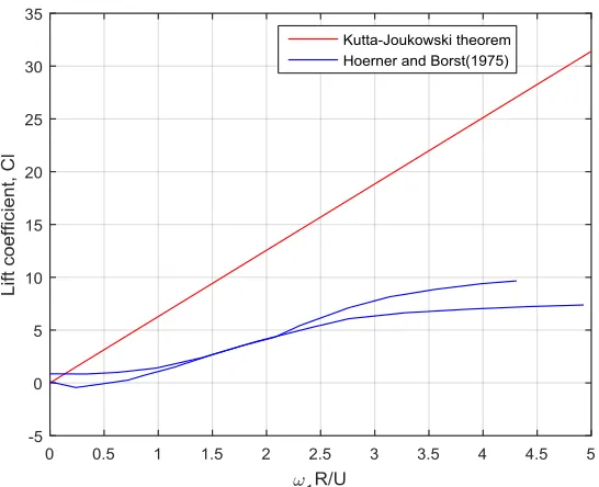
The Kutta-Joukowski lift theorem predicts a value forCl which is generally higher than

ex-perimental results suggest. The discrepancy is primarily due to viscous effect. However, the measuredClis in accordance with the theoretically predicted at small speed ratios, ωR_U (rolling

Fig. 4.2. Lift force of a rotating cylinder as a function of speed ratio

here values for Cl predicted by Kutta-Joukowski’s lift theorem are only used in cases with

small rolling frequencies. The following lift forces and moments are calculated:

FLy = Z 0.5L

−0.5L

ρUz(x)Γdx= Z 0.5L

−0.5L

ρ

h

−(U3−Ω2x) i

πDΩ1

D

2dx (4.67)

FLz = Z 0.5L

−0.5L

ρUy(x)Γdx= Z 0.5L

−0.5L

ρ

h

−(U2+ Ω3x) i

πDΩ1

D

2dx (4.68)

MLy = Z 0.5L

−0.5L

ρUy(x)Γxdx= Z 0.5L

−0.5L

ρh−(U2+ Ω3x) i

πDΩ1

D

2xdx (4.69)

MLz= Z 0.5L

−0.5L

ρUz(x)Γxdx= Z 0.5L

−0.5L

ρh−(U3−Ω2x) i

πDΩ1

D

2xdx (4.70)

4.1.8 Transformation of coordinate system

U3are computed at each time step. Based on the previous step’s rotation sequence of the coor-dinate system, the translational velocities are transformed from the local coorcoor-dinate system to the global system (Beeker et al., 1993):

˙

X =U1cos(θ) cos(ψ) +U2(−cos(φ) sin(ψ) + sin(φ) sin(θ) cos(ψ)) +U3(sin(φ) sin(ψ) + cos(φ) sin(θ) cos(ψ))

(4.71)

˙

Y =U1cos(θ) sin(ψ) +U2(cos(φ) cos(ψ) + sin(φ) sin(θ) sin(ψ)) +U3(−sin(φ) cos(ψ) + cos(φ) sin(θ) sin(ψ))

(4.72)

˙

Z =−U1sin(θ) +U2(−sin(φ) cos(θ)) +U3(cos(φ) cos(θ)) (4.73)

4.2

Comparison of dropped cylindrical objects

us-ing 2D theory and 3D theory

Fig. 4.3. Comparison of simulated trajectories of dropped cylinder at drop angle45o _with variance of Xt using 2D theory in Aanesland (1987) and new 3D theory withVroll= 0

4.3

Study of factors influencing trajectories

A drilling pipe model from Aanesland (1987) is selected as the dropped cylindrical object in this study. A list of possible factors to influence the 3D trajectory of dropped object are shown in Table 4.1.

Table 4.1: List of factors to study

Influencing Factors Unit Range

Drop angle (θ0) degree 0-90

Normal drag coefficient (Cdz) 1.0-1.2

Binormal drag coefficient (Cdy) 1.0-1.2

Rolling frequency (Vroll) rad/s 0-0.1

normal and binormal drag coefficients are supposed to be in the subcritical Reynolds num-ber range (about 1000-10000) where their values vary between 1.0 and 1.4 (Hoerner, 1958). But the numerical tests indicated that a smaller drag coefficient produced better trajectories to match experimental results, so only the range between 1.0 and 1.2 is studied. The comparison betweenX −Z plane trajectory from 3D simulations with drop angles30o, 45o and60o and corresponding experimental envelope is shown in Figs. 4.4-4.6.

Non-dimensional trailing edge position, Xt=|xt/L| =0.4 is used for cases with drop angles 30o and45o. As mentioned in Aanesland (1987), for greater drop angles, a largerXtshould be used. Therefore, Xt=0.5 is used for cases with drop angles larger than60o. Also, an ini-tial rolling frequency is assumed to be 0.05 rad/s. For each drop angle, the trajectories with different z directional drag coefficients, Cdz=1.0, 1.1 and 1.2 are simulated and presented in

Figs. 4.4-4.6, respectively. All the trajectories show a similar trend. However, a larger drag coefficient,Cdzspreads the trajectory in positiveX-direction potentially because the increased

resistance force slows the movement of dropped objects inZ-axis. Figs. 4.4-4.6 also indicate thatCdz=1.0 can produce a more reasonable trajectory if compared with the experimental

en-velope (Aanesland, 1987).

The selection of different drag coefficientCdy could affect the simulated trajectory in the X-Z

plane. Herein, various values are used, that is 1.0, 1.1 and 1.2. The corresponding trajectories are presented in Figs. 4.7-4.9. The trajectories almost overlapped. Therefore the influence of

Cdyon the motion inX−Z plane may be ignored.

The effect of drag coefficient Cdy on the transverse motion in the Y-Z plane is studied and

presented in Figs. 4.10-4.12. WhenCdy increases from 1.0 to 1.2, trajectory and landing point

tend to be pulled towards to the origin. With a drop angle of30o, the difference of landing point atCdy=1.0 and 1.2 reaches 0.14m which means the landing point is very sensitive to changes in

Cdy. With increasing drop angle, the difference of landing point atCdy=1.0 and 1.2 decreases

to 0.10m and 0.02m respectively. See Fig. 4.11 and Fig. 4.12. So it can be concluded that the sensitivity of dropped cylinders to the change ofCdydecreases with increases in drop angle.

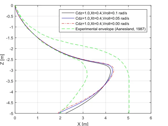
In order to consider the effect of rolling frequency, the corresponding trajectories are plotted in Figs. 4.13-4.15. All simulated trajectories are in good agreement with the experimental en-velope. The trends of the simulated trajectories and landing points for a drop angle at 30o are different when rolling frequency varies between 0 to 0.1 rad/s. For vanishing rolling fre-quency, 0 rad/s, the obtained trajectory follows the sketch given in Fig. 2.1(e). At a larger rolling frequency of 0.05 rad/s, the landing point moves to the left. Further increasing the rolling frequency to 0.1 rad/s, the simulated trajectory becomes close to sketch in Fig. 2.1(a). In addition, different rolling frequencies can cause some variation in the trajectory when the drop angle is less than45o, as indicated by Figs. 4.13 and 4.14. However, such difference seems less significant for cases with drop angles larger than45o_{, as indicated by Fig. 4.15.}

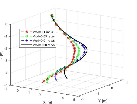
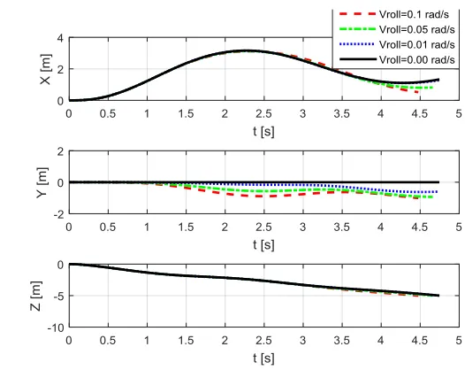
Fig. 4.16 presents an overview of 3D trajectories with different rolling frequencies: 0 rad/s, 0.01 rad/s, 0.05 rad/s and 0.1 rad/s. A comparison of time domain translational motions inX, Y

andZdirection is shown in Fig. 4.17.

Fig. 4.16. Simulated 3D trajectories with variance ofVroll at drop angle30o, Xt=0.4,Cdy=1.0,

Fig. 4.17. Simulated time domain translational motions (a) in X-direction (b) in Y-direction (c) in Z-direction (from top to bottom)

It should be noted that larger rolling frequencies causes the cylinder to hit the bottom slightly sooner, as indicated by the reduced total duration time t(s) listed in Table 4.2. Further, with increasing rolling frequency but fixed drop angle30o, the landing point approaches theZ-axis through the origin. However, it moves further inY direction (increasing Y). The shorter drop time associated with increased rolling frequency results in a larger terminal velocity at seabed in Z direction as indicated the Z directional component of terminal velocity,VtZ in Table 4.2.

More details about the terminal velocity and orientation of the dropped cylinder is recorded in Table 4.2.

Note: 1,VtX,VtY,VtZ are the components of terminal velocity at seabed in X, Y and Z direction. φt,θt,ψt are

orientation angles at seabed

2,Vttis the total terminal velocity at seabed calculated as:Vtt=

p

V2

tX+VtY2 +VtZ2

Multiple simulations have been carried out to investigate the excursion distributions and land-ing points on the bottom. The initial drop angle is varied from0o_to90o_{with an uniform}

Table 4.2: Excursion distribution for drop angle30o

Case number 1 2 3 4

Rolling Frequency(rad/s) 0 0.01 0.05 0.1

X(m) 1.33 1.31 0.99 0.58

Y(m) 0.00 -0. 18 -0.82 -0.99

t(s) 4.746 4.746 4.694 4.544

VtX(m/s) 0.906 0.772 0.263 -0.665

VtY(m/s) 0.000 0.200 -0.113 -0.482

VtZ(m/s) -1.150 -1.150 -1.091 -0.966

Vtt(m/s) 1.464 1.399 1.128 1.268

φt(rad) 0.000 0.110 0.279 0.448

θt(rad) 0.199 0.211 0.238 0.187

ψt(rad) 0.000 0.497 0.423 0.430

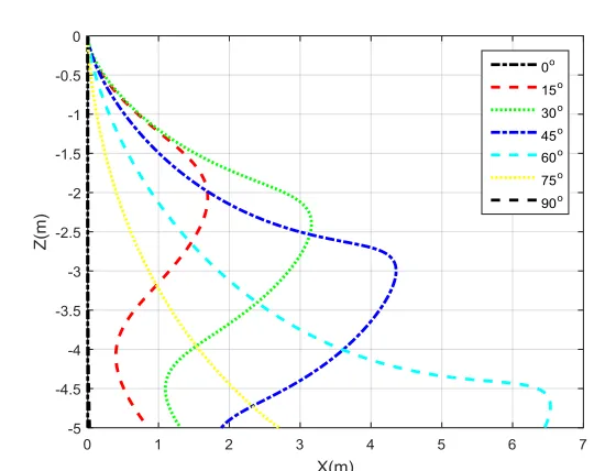
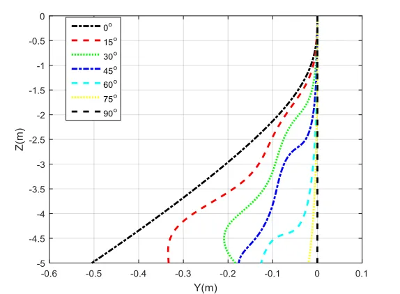
drop angles from60oto90o, X tends to decrease again. In Fig. 4.19 with drop angles increase from0oto90o, theY directional excursion decreases from 0.5m to 0m. Maximum excursion in

Y-direction occurs for a drop angle of0o.

Fig. 4.19. Simulated Y-Z plane trajectories with drop angle from0o_to90o_{,Cdy=1.0, C} dz=1.0, Vroll=0.01 rad/s

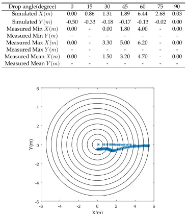
Table 4.3 provides the simulated data forXandY directional excursions of the landing points at different drop angles and compares them with corresponding statistical experimental data. Minimum value, mean value, and maximum value are taken from Aanesland (1987). All the simulated data are close to the experimental data range . Both numerical and experimental results found that the data show the maximum X directional excursion of the landing point occurring for a drop angle60o_{.The total excursion distribution at 5 meter water depth is plotted}

in Fig. 4.20 and 4.21 . The excursion radius R represents the distance from the landing point to the Z-axis and is defined by:

Table 4.3: Excursion distribution at drop angle30o

Drop angle(degree) 0 15 30 45 60 75 90

SimulatedX(m) 0.00 0.86 1.31 1.89 6.44 2.68 0.03

SimulatedY(m) -0.50 -0.33 -0.18 -0.17 -0.13 -0.02 0.00

Measured MinX(m) 0.00 - 0.00 1.80 4.00 - 0.00

Measured MinY(m) - - -

-Measured MaxX(m) 0.00 - 3.30 5.00 6.20 - 0.00

Measured MaxY(m) - - -

-Measured MeanX(m) 0.00 - 1.50 3.20 4.70 - 0.00

Measured MeanY(m) - - -

-X(m)

-6 -4 -2 0 2 4 6

Y(m

)

-6 -4 -2 0 2 4 6

X(m)

0 1 2 3 4 5 6 7

Y(m

)

-0.8 -0.7 -0.6 -0.5 -0.4 -0.3 -0.2 -0.1 0

Fig. 4.21. Excursion distribution at 5m water depth with drop angles from0oto90o,Cdy = 1.0, Cdz= 1.0, Vroll= 0.01rad/s, local view(Y axis scale enlarged)

A closer view of landing point distribution is shown in Fig. 4.21. Excursion in X-direction are more significant than in Y direction.

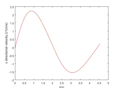
4.3.1 Study of translational and rotational motions

7 6 5 4 3 2 1 0 -1 X [m] -2 -3 -4 -5 -6 -7 -7 -6 -5 -4 -3 -2 Y [m] -1 0 1 2 3 4 5 6 -5 -4 -3 -2 -1 0 7 Z [m] Cdz=1.0,Xt=0.3,Vroll=0.1 rad/s

Fig. 4.22. 3D Simulated orientation and trajectory for drop angle30o

t(s)

0 0.5 1 1.5 2 2.5 3 3.5 4 4.5 5

x direction al ve locity,U1(m /s) -2 -1.5 -1 -0.5 0 0.5 1 1.5 2 2.5

t(s)

0 0.5 1 1.5 2 2.5 3 3.5 4 4.5 5

y

dire

ctional

ve

locity,U2(m

/s)

-0.7 -0.6 -0.5 -0.4 -0.3 -0.2 -0.1 0

Fig. 4.24. The velocity time series of sway

t(s)

0 0.5 1 1.5 2 2.5 3 3.5 4 4.5 5

z

dire

ctional

ve

locity,

U3(m

/s)

t(s)

0 0.5 1 1.5 2 2.5 3 3.5 4 4.5 5

rolli

ng

freque

ncy,

1

-0.25 -0.2 -0.15 -0.1 -0.05 0 0.05 0.1 0.15 0.2 0.25

Fig. 4.26. The velocity time series of roll

t(s)

0 0.5 1 1.5 2 2.5 3 3.5 4 4.5 5

pitching

frequen

cy,

2

-0.8 -0.6 -0.4 -0.2 0 0.2 0.4 0.6

t(s)

0 0.5 1 1.5 2 2.5 3 3.5 4 4.5 5

yaw

ing

frequen

cy,

3

-0.6 -0.4 -0.2 0 0.2 0.4 0.6

Fig. 4.28. The velocity time series of yaw

t(s)

0 0.5 1 1.5 2 2.5 3 3.5 4 4.5 5

rotationa

langle

around

x

ax

is,

(rad

)

t(s)

0 0.5 1 1.5 2 2.5 3 3.5 4 4.5 5

rotationa langle around y ax is, (rad ) -0.4 -0.3 -0.2 -0.1 0 0.1 0.2 0.3 0.4 0.5 0.6

Fig. 4.30. Time series of the Euler angle in pitch direction

t(s)

0 0.5 1 1.5 2 2.5 3 3.5 4 4.5 5

rotationa langle around z ax is, (rad ) -0.6 -0.5 -0.4 -0.3 -0.2 -0.1 0 0.1 0.2 0.3 0.4

4.4

A more genereal three-dimensional (3D)

the-ory for dropped objects with nonzero LCG

4.4.1 Rigid body kinematics

In case where the longitudinal center of gravity (LCG) does not coincide with the origin, the ac-celeration of the body at the mass center,G, in terms of the body fixed system can be expressed by

~

VG =V~o+Ω~o×R~G (4.75)

~aG=~ao+~Ω˙o×R~G+~Ωo×(~Ωo×R~G) (4.76)

Substituting Eq. (4.10) into Eq. (4.76) yields,

~aG= ( ˙u−vr+wq−xG(q2+r2) +yG(pq−r˙) +zG(pr+ ˙q))~i + ( ˙v+ur−wp+xG(pq+ ˙r)−yG(p2+r2) +zG(qr−p˙))~j + ( ˙w−uq+vp+xG(pr−q˙) +yG(qr+ ˙p)−zG(p2+q2))~k

(4.77)

4.4.2 Rigid body dynamics

A rigid body consists of a set of material points with massesmilocated at the vector positions

~

Ri =xi~i+yi~j+zi~k. The total mass of the body ism= Σimi. The position of the center of mass

is determined byR~G = _m1ΣimiR~i. The time rate of the linear momentum for the rigid body

may be expressed as:

d dt

h

Σmi(V~o+~Ωo×R~i) i

= (Σmi) dV~o

dt +

d dt

h

~

Ωo×(ΣmiR~i) i

= (Σmi) dV~o

dt +

˙

~

Ωo×(ΣmiR~i) +Ω~o× h

~

Ωo×(ΣmiR~i) i

=mh~ao+~Ω˙o×R~G+Ω~o×(~Ωo×R~G) i

=m~aG

(4.78)