Edge Enhanced Deep Learning System for Large-scale Video Stream
Analytics
M.Ali
1, A.Anjum
1, M.U Yaseen
1, A.R. Zamani
2, D.Balouek-Thomert
2, O.Rana
3, and M.Parashar
2 1University of Derby, UK
Email:
{
m.ali, a.anjum, m.yaseen
}
@derby.ac.uk
2
Rutgers University, NJ, US
Email:
{
alireza.zamani, daniel.balouek, parashar
}
@rutgers.edu
3
University of Cardiff, UK
Email:
[email protected]
Abstract— Applying deep learning models to large-scale IoT data is a compute-intensive task and needs significant com-putational resources. Existing approaches transfer this big data from IoT devices to a central cloud where inference is performed using a machine learning model. However, the network connecting the data capture source and the cloud platform can become a bottleneck. We address this problem by distributing the deep learning pipeline across edge and cloudlet/fog resources. The basic processing stages and trained models are distributed towards the edge of the network and on in-transit and cloud resources. The proposed approach performs initial processing of the data close to the data source at edge and fog nodes, resulting in significant reduction in the data that is transferred and stored in the cloud. Results on an object recognition scenario show 71% efficiency gain in the throughput of the system by employing a combination of edge, in-transit and cloud resources when compared to a cloud-only approach.
I. INTRODUCTION
Internet of Things (IoT) devices such as sensors, video cameras and smart objects [1] act as the basic building blocks of smart cities and autonomous vehicles. The expo-nential growth and availability of these devices is producing a tremendous amount of data in zettabytes. As a result of these IoT deployments, large data volumes need to be transmitted via a (public) network to the analytics platform. In video analytics, a single video camera can produce about 25-30 frames/second. In HD and FHD cameras an 8-bit uncompressed RGB frame amounts to about 553 Mbps and 1.24 Gbps for a one minute video, respectively. With the advent of 4k and 3D video cameras, this size is likely to grow exponentially. By 2021, video traffic will account for about 82% of the whole IP Internet traffic, as estimated by Cisco Global [2]. Developers and engineers are facing the challenge of providing on time analytics of video data to support public safety and security from video cameras. Cloud computing is not efficient enough to support prompt analytics of such video data [3]. Video Analytics based on edge computing is the only feasible approach to cater low latency requirement for large-scale video streams [4].
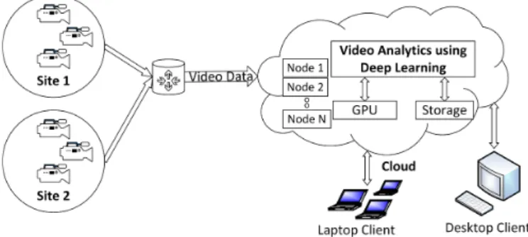
Fig. 1. Traditional Cloud based Video Stream Analytics
Traditionally video data from data sources is transferred to the cloud where data analytics takes place, and results are sent back to the client as shown in Fig.1. The traditional model suffers from high latency and network bandwidth use, as all the data has to be transferred to the cloud for analytics. Video analytics is described as an autonomous understanding of the events or actions occurring in a video feed [5], and is still in its infancy compared to other forms of analysis. Two approaches to video analytics are (i) centralized and (ii) edge based architecture as mentioned in [6]. In a centralized approach data from video cameras are routed to a centralized cloud where all of the analytics takes place, whereas in an edge-based architecture part of the analytics is performed near the source of data and partly on the centralized cloud. Most of the existing intelligent video analytics (IVS) systems are based on centralized approach and assume the video data to be readily available in proximity to where analytics takes place. However, in reality, the video data has to be transported from a source which may involve moving the data through several network hops to reach the destination where it is stored and analyzed.
With the success of deep learning, video analytics using deep learning is increasingly being employed to provide accurate answers to object classification particularly with convolutional neural network (CNN) [7]. However
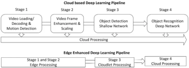
perform-Fig. 2. Deep Learning Pipeline for Object Recognition
ing analytics using deep learning is a complex task with high demand put on the performance and the accuracy of results. Deep learning algorithms often use cloud computing for training and inference. With the exponential growth of video data from cameras, the traditional cloud computing paradigm is not able to meet the Quality of Experience (QoE) demands often associated with network latency and Round Trip Time (RTT) constraints. Moreover, an increase in data from video cameras leads to an increasing cost of resources on a centrally managed cloud [8].
Unlike the use of data prediction techniques on batch data, video analytics is a complex problem and can often logically be decomposed into stages. For example, object recognition in videos can be decomposed into stages of motion detection, frame enhancement, object detection, and recognition. A typical Cloud-based deep learning pipeline for object recog-nition and the proposed edge enhanced decomposition of the pipeline is shown in Fig.2. It consists of four stages marked as S1-S4. In cloud-based systems, typically all of the stages are executed on the cloud particularly if the source producing the data is on a different network than the client. In this work, we split the deep learning pipeline by using edge computing resources to improve the performance of the video analytics system while keeping the accuracy intact.
Our main contributions are:
• Design and development of an edge inspired
infrastruc-ture for high-performance video streams analytics.
• Distribution of the deep learning pipeline stages across
the edge, in-transit and cloud resources to bring the benefits of low latency, reduced bandwidth costs and improved performance for object inference.
• To provide a scalable architecture which could
effi-ciently scale to a large number of video cameras by utilizing hardware resources including multiple edges, in-transit and cloud nodes to provide high-performance analytics.
The rest of this paper is organized as follows. In section II we describe state of the art in edge computing and computer vision. In section III, we propose our system architecture for edge enhanced deep learning and how it can scale to many edge and in-transit nodes to provide parallel and sequential processing of the video streams. In section IV, we discuss the decomposition of an object recognition scenario and develop a data pipeline model for video streams. We also briefly describe the training setup of the neural network
used for object recognition in this section. In section V and VI we discuss the experimental setup and the results obtained respectively. Section VII include conclusions and future directions of the work.
II. RELATED WORK
Existing efforts in video surveillance have relied on the human operator manually watching camera feeds and press-ing an alert button in case of an event. However, security personnel can hardly remain alert for monitoring tasks after 20 mins [9]. Recently intelligent video analytics systems (IVS) with the aim to analyze video streams without human intervention have emerged which provide constant analysis of a scene [10]. Most of the existing work on intelligent video analysis is based on centralized architecture using a storage-analyze cloud model such as [11] where the data is first transported and stored in the cloud. The analytics is then performed on the stored data using job scheduling [12]. The post analytics of video data is a time consuming process and can often take hours.
Deep learning has seen unprecedented success in recent years for complex tasks such as speech and facial recogni-tion. CNN is a deep learning model which has brought a breakthrough in image, video and audio classification prob-lems. In [13], the authors used CNN for large-scale video classification. The training and inference of deep learning models are performed by using cloud services [8]. With the proliferation of IoT devices, analytics on the cloud can suffer from slow response times mainly due to network delays and round trip times. Due to high data volumes from IoT, data
has a stronggravitywhich indicates the difficulty of moving
a mass amount of data over the network. A viable approach is to move the analytics towards the data source instead. Consequently, edge and fog Computing [14] are proposed as new paradigms, where data analytics takes place at the network edge to minimize the cloud workload, to improve the response times and to reduce the cloud storage. Current work in edge computing focuses on reducing latency and bandwidth from edge/cloudlet to cloud such as in Gigasight [15] by running computer vision algorithms on the cloudlet and sending the resulting reduced data (output, recognized objects) to the cloud. An edge based system utilizing edge and cloud computing include [16]. Another important work in this regard is [17], which focuses on video analytics using edge and in-transit resources with a deadline time for each job. Some works such as Yaseen et al. [18] employ Graphics Processing Unit (GPU) to accelerate the video processing tasks to reduce the computational complexity involved in video stream decoding and processing. Another GPU based video analytics system on the cloud [19] is capable of analyzing recorded streams of video data from a cloud or storage server. An operator specifies the video file and search criteria to a client program; video analytics is then performed on the cloud and results are returned to the operator after some time. However, these system only considered video analytics using a centralized architecture.
Video Sources Stream Preprocessing Edge Node1 Stream Preprocessing Edge Node2 Stream Preprocessing Edge Node3 Stage 1: Preprocessing E dg e Nodes P ar allel Pr ocessing
Stage 2: In-Transit Analysis
Cloudle t Node s P ar allel Pr ocessing
Data MovementReduces storage, processing and bandwith requirement. Edge Processing In-transit Cloudlet Processing Cloud Processing
Cloud Node 1
Stage 3: Final Processing
GPU Storage Cloud Node N GPU Storage Video Streams C Cam 1 C Cam 2 C Cam 2 Site 1 C Cam 1 Site 2 Stream Preprocessing
Edge Node N Horizontal Scalability for Sequenal Processing
Previous Tier Next Tier Node 1 Node N Node 1 Node N Node 1 Node N
Loca on A Locaon B Locaon N
Node 1 Master Node V er cal Sc alabili ty f or P ar allel Pr ocessing Pr e vious Tie r Ne x t T ier Node N
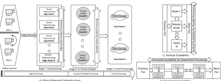
a) Edge Enhanced Infrastructure b) Horizontal Scalability
c) Vertical Scalability
Fig. 3. Edge Enhanced Deep Learning Architecture with Horizontal and Vertical Scalability for Video Stream Analytics
As evident from the above discussion, existing state of the art in video analytics focus is to provide accurate results using both shallow networks and deep learning models. These systems assume the video data is readily available for analytics while the transfer cost and network latency from source to destination is not considered. Few systems analyz-ing video streams from cameras also assume the streamanalyz-ing data has been stored in the cloud. In contrast to that, we assume the video data is continuously being streamed from IoT devices and discuss the challenges arising in this scenario. Our focus in this paper to improve the performance of the deep learning pipeline for video analytics by utilizing edge computing paradigm. To the best of our knowledge, this is the first time an edge computing based deep learning pipeline distribution for efficient video analytics has been proposed. The proposed system can be tailored to meet the demand for real-time applications other than video analytics such as speech recognition and anomaly detection.
III. EDGEENHANCEDSYSTEMARCHITECTURE FOR
VIDEOANALYTICS
The proposed system architecture consists of three logical tiers namely edge, cloudlet and the cloud as shown in Fig.3a. Video streams from data sources pass through the edge and cloudlet tiers to reach the destination cloud. Cloudlet or fog node is an in-transit node placed between the edge and the cloud. Tiers can scale in vertical and horizontal direction. In Vertical Tier Scalability (VTS), a tier may contain one or more computational nodes to form a cluster as shown in Fig.3c. Vertical tier nodes are connected with Local Area Network (LAN) in a close vicinity forming a compute cluster which is managed by a master node. In Horizontal Tier Scalability (HTS), a tier can extend in the horizontal direction with a set of vertical clusters at a certain physical distance from each other as shown in Fig.3b. The vertical tier scalability provides parallel processing of the video streams, and horizontal tier scalability provides sequential processing of the streams in a single logical tier. This scalability can
be adapted to the available hardware resources and the specific analytics problem. It allows parallel and sequential processing of data in three tiers. The master node of each tier in VTS receives input from the previous tier and distributes the load among available tier nodes. Tier nodes in VTS work in parallel reducing the time to process the overall video data. In VTS case, if there are 500 video frames to process and a tier consists of two nodes, then each node may process 250 frames in parallel. At the network edge, video cameras continuously stream time series video data to the network. The video data is moving to the cloud in the horizontal direction. As the data is in-transit, analytics is performed at the intermediate nodes at the edge and cloudlet nodes. In smart cameras, we can program the cameras to broadcast the video to the network only when there is some motion detection. In this case, edge tier includes the camera device and the immediate edge node. In simple devices, such as sensors, we may only forward the data to the cloud if the temperature exceeds a certain value. These devices work on rules which are specified by the user. One such tool is Krikkit [20] which allows edge devices to be programmed by rules specified using web services rather than programming each of the network nodes manually. However, for video analytics, the problems of vehicle tracking, object recognition and semantic segmentation are not tractable with simple rules, due to the complexity of the problems. By employing CNN, a deep learning model, we distribute the data pipeline across network nodes. Initially, the CNN models are trained on the cloud, and the resultant models are saved. The saved models are then transferred and distributed over cloudlet and cloud resources for object inference. The edge resources are used for basic processing stages. By overlapping the deep learning pipeline stages over edge, in-transit and cloud resources, the deep learning pipeline can be executed in parallel to improve the performance of the overall system. The numbers of nodes in each tier may vary depending on the commodity hardware availability and the application requirements. Total computational nodes on the network will
be the sum of the edge, cloudlet and cloud resources. By using infrastructure in Fig.3, we can transform the low-value density of video data into high-value density data before feeding this data to the cloud resulting in improved response times, reduced bandwidth and storage requirements on the cloud. For object recognition, we define the value of the data as high if the video frame contains an object or low otherwise. The video data is pushed from the video sources to in-transit resources and the central cloud using software-defined networking (SDN) [21] such as OpenFlow [22]. SDN is a design methodology for personalized networking and provides the flexibility to deploy custom work-flows on com-modity hardware by programming the control plane. As the data is in transit, it can be filtered by the edge and in-transit resources. The filtration process can transform the video streams from a low-value density to a high-value density data before being fed to the cloud for final processing. Fig.3 shows the reference architecture for a constant streaming video analytics which can be modified to a specific video analytics problem and the available hardware resources to generate an application specific architecture (ASA). SDN can then be used to realize the physical configuration of the ASA consisting of edge, cloudlet and cloud nodes.
IV. EDGEENHANCEDDEEPLEARNINGMODEL
Researchers have traditionally relied on handcrafted fea-tures to solve computer vision problems with limited success. Recently with the advent of deep learning, problem features can be automatically learned by the deep learning algorithms such as CNN. Deep learning has achieved promising results which equal to or exceed human performance in computer vision problems [23]. In video analytics domain, problems such as object recognition and segmentation can be decom-posed into a cascade of simpler problems. For example, object recognition is a complex video analytics problem and consists of the following stages
• S1. Frame Loading/Decoding and Motion Detection:
Video frame from the camera source is first loaded and decoded in memory. The video frame is then passed to a motion detector where it is compared with the pre-vious frames for differentiation. Video sources such as Closed-circuit television (CCTV) cameras continuously produce video data even if there is no change in frames; motion detection is usually employed to reduce the input data.
• S2. Preprocessing: Includes basic enhancements such
as conversion to binary Image, histogram equalization, and scaling where an image is downscaled or upscaled according to the algorithm requirement.
• S3. Object Detection and Decomposition: Process video
frame into single objects, a video frame may consist of more than one object. Usually, the frame is decom-posed into individual objects, and then each object is individually detected. The detection of object orienta-tions/landmarks in a bad light or low light conditions is also considered in this stage.
• S4. Object Recognition: The video frame is passed
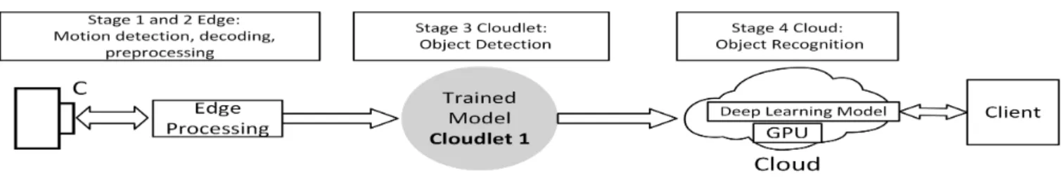
through a deep learning model for object recognition. The stages above can be distributed among edge, cloudlet and cloud resources in varied ways which determine the performance of the system. In general for a video analytics problem, the work can be divided into three phases. In the first phase, the deep learning pipeline is decomposed into logical stages. For each stage, one or more computational tasks are determined. In the second phase, stages based on machine learning are trained on the cloud. In the third phase, the stages are distributed on the physical network nodes using SDN. The decision to run the trained model on cloud or cloudlet can affect the performance of the overall system. The decision strategy of running trained models on cloud or cloudlet is discussed in section IV-B. In general, we perform non-compute intensive stages on the edge tier and more compute-intensive stages on the in-transit and cloud tiers. For object recognition case, the distribution of stages over network resources is shown in Fig.4. For S1 and S2, edge tier can be used. Edge tier is defined as consisting of the data sources (cameras) and the edge nodes. For S3 machine learning model to detect the object is run on the cloudlet node. For S4, the trained deep learning model is run on the cloud to perform the compute-intensive work of object recognition. If there are more than one deep learning models for these stages, we need a way of mapping the deep learning models onto our cloudlet and cloud nodes. In general, if we denote the deep learning pipeline for a specific video analytics problem by letter ’P’, the number of stages for the problem set P is
P ={S1, S2, S3...SN} (1)
SN is the final stage number, and the set P denotes all the
stages of a problem P. It consists of two types, basic stages and machine learning stages. Basic stages do not involve a machine learning model for processing. For each stage, we
may have one or more tasks given as a setTSi
TSi=T1, T2, T3, . . . TN (2)
where ’i’ in Si denotes a stage number. Total tasks for all
stages is given by TtS= N X n=1 TSn (3)
Each task in a stage performs some transformation on the input frame resulting in an output frame given by the following equation
G(x, y) =T(F(x, y)) (4)
G(x, y)indicates the output pixel value at location x, y and
F(x, y)indicates the input pixel value at location x,y. The ’T’ indicates the transformation function which is applied to all the pixels of the frame. For basic processing stages, the trans-formation function could be an image smoothing/sharpening, noise reduction, histogram equalization and or image scaling.
Fig. 4. Edge Enhanced Deep Learning for Object Recognition Scenario
For deep learning stages, the transformation function will be a deep learning model.
If there are more than one deep learning stages, deep learning models to run on each node is given by M
M =DL(SN)/N (5)
DL is a function which takes the total number of stages in a problem and returns the number of deep learning models in the problem. N is the number of cloudlet and cloud nodes. If M is more then one, it means we need to execute more than one model on either cloudlet or cloud node. Due to processing and storage constraints, we do not consider edge as a candidate for deep learning models. Deep models may or may not have a dependency; dependent models must be executed in a sequence to yield correct results. Detection of an object is a precursor step to object recognition, therefore object recognition model is dependent on the object detection model and must be executed after it to conform with the serial execution requirement. An example of independent models is a driver recognition scenario. The semantic recognition of the driver and the vehicle may need two deep learning models without dependency; it does not matter whether a person is recognized first or the vehicle. We discuss three strategies to decide the execution of models on network nodes given in section IV-B
A. Data Pipeline Model
The inference is to be performed on the video streams coming from cameras. We denote the set of video cameras as
CN ={C1, C2, . . . CN} (6)
where N is the total number of video cameras. Each of these video cameras is producing data at N frames per second; each camera frame rate is denoted by
CN f ps={F1, F2, F3, F4. . . FN} (7) Each frame is considered a job to be processed by the deep learning model. Number of jobs produced cameras with same frame rate per second will be
CN jps=CN f ps∗M (8)
whereCN f ps is the number of frames per second for camera
N and M is the number of cameras with the same frame rate.
Total number of jobs produced by all camera in one second will be JT jps= N X n=1 CN f ps∗N (9)
where CN f ps denotes the camera with unique frames per
second and N is the number of cameras with the same frame rate. The time cost to process each job with algorithm A will be
Cja=At+Tt (10)
where At is the algorithm time to process the job and Tt
is the network time to transfer the record from source to destination. Total cost to process all the jobs with algorithm A will be
CT ja=JT jps∗Cja (11)
whereJT jpsis the total number of jobs andCja is the cost
time for each job. We also define a percentage gain to show the efficiency of a setup S in terms of time and cost of a reference cloud setup.
Gs= (CT ja(c)−CT ja(s))∗100/CT ja(c) (12)
whereCT ja(s)is the total cost to process all jobs on a setup
S and CT ja(c) is the cost to process all the jobs on cloud
setup. We will use the Gain to compare our approach with the traditional cloud model and to prove the efficacy of the proposed system.
B. Model Decomposition Decision Strategy
The deep learning pipeline consist of 1) deep learning models and 2) basic processing stages. For multiple stages, the choice of running the deep learning model on the Cloudlet or Cloud is a critical decision to be made. Depend-ing on the problem requirement, it can largely influence the response time and bandwidth/storage costs between network resources. Model selection decision on network nodes is based on the model algorithm time and the volume of the data to be processed by the model. To make the decision easier, we propose three strategies as following:
• Model Time (MT): Based on the inference time each
model takes, we decompose the models on the edge, cloudlet, cloud tiers by observing the available hardware and application requirements. Intuition may lead us to run the compute-intensive model on the Cloud, however, if it also has a more capacity to filter low-value density data, it might be appropriate to run it on the cloudlet
Algorithm 1 Model Time based Node Allocation
Input: Models
Output: CloudNodes,CloudletNodes
Initialisation :
If its a single model schedule it on cloud
1: if (Models.size()==1)then
2: CloudNodes.first().assignModel(Models.first))
3: return CloudNodes, CloudletNodes
4: end if
Find model time for each model
5: Map{Model,Time} modelTimeMap
6: for(i= 1toM odels.size)do
7: time=Models[i].getAlgorithmTime()
8: modelTimeMap.set(Models[i], time)
9: end for
Sort the model time map based on time
10: if (strategy=highTimeOnCloud)then 11: sortAscending(modelTimeMap, time) 12: end if 13: if (strategy=LowTimeOnCloud)then 14: sortDescending(modelTimeMap, time) 15: end if
Allocate the models on cloudlet and cloud node
16: for(i= 0toCloudletN odes.size())do
17: m=modelTimeMap.getModel(i)
18: CloudletNodes.assignModel(m)
19: end for
Check if there are models to be assigned to Cloud
20: if (modelT imeM ap.size() > CloudletN odes.size())
then
21: for(i= 0toCloudN odes.size())do
22: cloudletSize=CloudletNodes.size()
23: m=modelTimeMap.getModel(cloudletsize+i)
24: CloudNodes[i].assignModel(m)
25: if((cloudletsSize+i)> modelT imeM ap)then
26: Break
27: end if 28: end for 29: end if
30: return CloudN odes, CloudletN odes
to reduce the network bandwidth and to save the cloud costs. Algorithm for this strategy is given in Algorithm IV-B.
• Frequency Sampling: In this strategy, we estimate the
number of classes in the video streams. In case of object recognition, two classes can be ”object-yes” and ”object-no”. Based on a statistical approach, count of all the classes is estimated and is used to schedule the model on cloudlet or cloud. For instance, if a dataset has more background objects, frequency-based sampling can be employed to detect and filter the background objects in the cloudlet. On the other hand, if the dataset has many foreground objects than background objects, it might be appropriate to run the deep learning
TABLE I
STORAGE SIZE AND PROCESSING DEADLINE Name Memory Storage(MB) Deadline(sec)
Edge 32 1
Cloudlet 64 2
Cloud 128 500
recognition model on both cloudlet and cloud to make the system efficient.
• Adaptive Strategy: This strategy observes the history of
the previous one hour, one day or one month record and switches the cloudlet and cloud nodes based on cloud saving, cloudlet cost-saving strategy. The saving cost may apply to energy, bandwidth and or storage saving. It is determined subjectively by the user based on analysis of the network and application requirements.
C. Deep Model Training
The deep learning training for object recognition was performed on the cloud platform. After the model was trained, it was saved in a file and used for object inference on video streams coming from the camera sources. For object detection, a pre-trained model was obtained from the OpenCV library [24]. It was not feasible to decompose the deep learning training towards the edge due to two reasons. Firstly, the training data was already available in the cloud. Secondly, as cloudlets and edge nodes are usually not near each other, distributing the training process on edge and cloudlet nodes may introduce a significant delay which may hamper the training process more than if it was being trained on a cloud. The deep learning training was performed on the cloud cluster with 8 compute cloud nodes using the University of Derby cloud. Each node in the cloud has a storage of 100 GB, 4 VCPUs and 16 GB RAM. The total video dataset size is 5GB. The first convolutional layer of CNN filters the frames with 96 kernels. The layer next to it has 256 kernels in it. The next three layers are convolutional with 384 kernels in them. All these layers end up to fully connected layers. The object recognition model was fully trained after about 1 hour and the trained model was saved on a disk storage.
V. EXPERIMENTAL SETUP
The experimental setup was created using OMNeT Sim-ulator. It is a discrete event simulator and provides accurate simulations for a wide variety of scenarios. Every effort was made to make the simulation as accurate as the real hardware. The experimental setup consists of video cameras, processing nodes and gateways (switches, routers) to transport data between hosts. The edge and in-transit nodes have limited memory storage space. When the memory buffer of an edge or in-transit resource is exceeded, it sends all the jobs in its current memory buffer to the next network hop and frees the space occupied. All processing nodes also associate a time deadline to each object recognition job in their current memory buffer under which a job should be completed. The storage space for the computational nodes
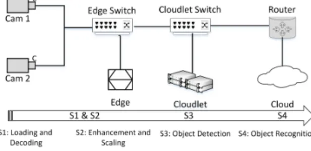
Fig. 5. Experimental Setup for Deep Learning Object Recognition
and their deadline time to process a job is given in Table I. If a network node is unable to process the job under its respective deadline time, the job is forwarded to the next hop in the network or rejected in case of a cloud. The experimental setup in Fig.5 depicts a subset of the proposed infrastructure given in Fig.3 and presents a sim-ple scenario to demonstrate the efficacy of the system.
A brief explanation of the nodes is given below.
Cam1 and Cam2 are video camera sources and are con-tinuously streaming video data of 20 and 10 frames per second respectively. The data is obtained from the video folder which consists of images of HD res-olution with an average size of 102Kb. Cam1
pro-duces about 2Mb of video data per second and
cam2 produces about 1Mb of video data per second.
Edge Switch moves data from video sources to edge or to the next network node. The decision of switching is based on the configuration being run. For instance in cloud only mode, it transfers all the video data to the next network switch, that is cloudlet Switch in our setup.
Cloudlet Switch decides to forward the packet either to the next network hop that is cloud Router or to the cloudlet. The decision is made based on the experiment and
config-uration being executed. Cloud Router is used to forward
video data from the data source network to the cloud network to reach the cloud. We assume the cloud resides on a network other than the rest of the nodes and is connected to the data sources network through a router.
Edge node does preprocessing of the data before
forward-ing the data back to the edge Switch. Edge Switch then forwards it to the next horizontal node. Edge node has a limited storage buffer for jobs. A job from the camera is first stored in the buffer of the edge node before it can be processed, the job is removed from the buffer after processing. The buffer size is fixed for all experiments. If the incoming jobs exceed the storage buffer of the edge node, processing is aborted and edge node forwards the unprocessed jobs to the next node in the network.
Cloudlet is an intermediate node which sits between the data sources and the destination cloud. It has more storage and processing capacity than the edge but equal to or fewer resources than the cloud. The cloudlet is used to perform inference for object detection. Video Data is transferred to the cloudlet node only in cloudlet-cloud and
edge-cloudlet-cloud mode. The storage capacity of the edge-cloudlet-cloudlet is fixed for all the experiments and is given in Table I. Likewise edge, if a cloudlet buffer is exceeded, it forwards the jobs to the next network hop without processing and frees its buffer storage. The Cloud performs the final processing and is the last network node for the data in transit from the video sources. The cloud runs a deep learning inference model for object recognition on every job which takes around 250ms in average. The storage capacity of the cloud is assumed to be sufficient for the experiments being conducted. The Internet Protocol (IP) address for the nodes was assigned automati-cally by the software. Nodes were connected to each other through communication links and ports. Ports are referred to as gates in the simulator and were manually configured for each node. All the nodes are placed from each other at a certain distance to introduce the delay in the communication links. Edge node is assumed to be closest to data sources, cloudlet is placed in-between cloud and the edge node and cloud is the furthest from data source. The communica-tion delay between edge Switch to cloudlet Switch and cloudlet Switch to cloud Router is 2ms and 4ms respectively. All the other network connections have a delay of 1ms. The experimental evaluation is performed using an object recognition use case because it needs deep learning models and has complex computational and data access require-ments. The experimental setup is used for evaluating the proposed system and producing the results. The frames from video cameras consist of images of High Definition (HD) quality with an average size around 103KB. The frames are of two types i) background frames and ii) foreground frames. Background frames only consist of background information while the foreground frames consist of an object with a background. In the dataset that has been used to evaluate the system, the ratio of foreground to background frames is 2:3, out of every 5 frames transferred, 2 consist of foreground objects and 3 have only background information. We associate foreground frames with a high value of 1 and background frames with a low value of 0. A video stream with all foreground frames will have a high-value density and video frames with a mix of background and foreground frames will have a low-value density. A continuous streaming video data is produced by the camera sources to emulate the real-life scenario. The edge, cloudlet and cloud nodes have been used to evaluate the distribution of deep learning pipeline for object recognition operations in real time on the streaming data.
VI. RESULTS AND DISCUSSION
The experiments were run for four software defined net-working (SDN) configurations namely i) Cloud Only (CO) ii) Edge-Cloud (EC) iii) Edge-Cloudlet-Cloud (ECC) iv) Edge-Cloudlet-Cloud with Filtration (ECCF). In all of the configurations, tests were performed for object recognition inference. No tests were performed for deep learning training as it was not distributed towards the edge and in-transit resources. For each SDN configuration, two experiments were run.
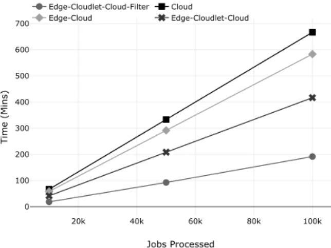
20k 40k 60k 80k 100k 0 100 200 300 400 500 600 700 Edge-Cloudlet-Cloud-Filter Cloud Edge-Cloud Edge-Cloudlet-Cloud Jobs Processed Time (Mins )
Fig. 6. Time to process 10k,50k,100K jobs on the four SDN configurations
Fig. 7. Time to process stages of an object recognition job in milliseconds (ms)
A. Experiment 1: Total time to process 10K, 50K, and 100K object recognition jobs
In the first experiment total time to process object recogni-tion jobs was measured and plotted. The experiment was run for 60 minutes and time was noted to process 10K, 50K and 100K jobs. In total 108,000 video frames were submitted to the system which amounts to about 10.6GB in size.
1) Cloud Only: The cloud only configuration is the tradi-tional approach and is used as the reference to compare and analyze the results with the other SDN configurations. In this setup, all the stages of the deep learning pipeline shown in Fig. 7 were executed on the cloud and results were obtained. For the first experiment using Cloud only configuration, the results are shown in Fig.6. It takes about 666 minutes (11 hours and 7 minutes) to process 100K jobs. During this time 100K total object recognition inference jobs were completed. The cost function for the total jobs defined in equation 11
is given belowCT ja=100000*400/1000=40,000s (11hrs and
6 mins) The actual time to process these records as shown in Fig.6 is 2 seconds more than the total cost function. This delay is attributed to transfer of the video data from video cameras to Cloud node.
2) Edge and Cloud Only: The experiments were repeated for edge and cloud only configuration. In this case stages S1 and S2 of Fig.7 were executed on the edge and S3 and S4 were run on the cloud. The results are shown in Fig.6. In this case, percentage efficiency gain is more than the Cloud only approach as distribution of stages S1 and S2 on the edge introduces parallel processing and reduces the time to process all the jobs.
3) Edge, cloudlet and Cloud Only: In this configuration all the network resources that are edge, cloudlet and cloud were employed to distribute the tasks among them. Stages 1 and 2 of Fig.7 were distributed on the edge node while stage 3 and stage 4 were distributed on cloudlet and cloud nodes respectively. The results are shown in Fig.6. It is more efficient than the Edge-Cloud approach as the object detection stage S3 which was being executed by the Cloud is transferred to the cloudlet. Since object detection is a compute intensive task, it took less time to process the overall jobs in Edge-Cloudlet-Cloud approach as increased parallelism for compute-intensive tasks lead to increase in percentage efficiency gain.
4) Edge, Cloudlet, Cloud with Filtration: It is same as edge, cloudlet and cloud configuration, however in this case we have filtered streams which fall under the filtering criteria. For example, streams with only background frames are a candidate for filtering as they do not contain any useful data to recognize the object. It is important to note in real video camera streams; not all the frames are of interest. In object recognition case, we can only forward the frames to the cloud in which an object has been detected by an object detection model. As object recognition is a compute-intensive task and consumes significant time, by filtering the streams at the cloudlet node, we were able to accelerate our system performance. As shown in Fig.6 it takes less time to process object recognition jobs in Edge-Cloudlet-Cloud-filter approach than in Edge-Cloudlet-Cloud approach. The percentage gain in ECCF case as compared to the cloud only and Edge-Cloudlet-Cloud approach is 71% and 54% respectively.
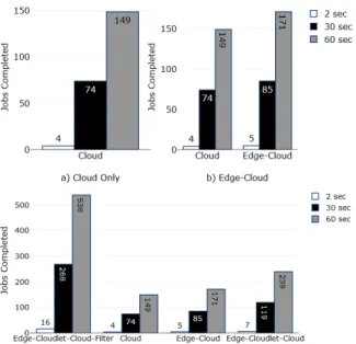
B. Experiment 2: Number of object recognition jobs com-pleted in window time of 2,30,60 seconds
For near real-time analytics, it is often more important to determine the number of object recognition jobs completed per unit time to aid in decision making and to provide timely control of events. To demonstrate this, we plot the chart for window time of t=2,30,60 seconds for all the four configurations as in experiment 1. The distribution of stages for the configurations were the same as Experiment 1.
1) Cloud Only: For the second experiment on the cloud, it can be seen in Fig.8a that only 4 jobs were completed in 2 seconds, 74 jobs in 30 seconds and 149 jobs in one minute. We use the cloud case as a reference to compare and evaluate results with the other configurations.
2) Edge and Cloud Only: In this case, edge and cloud nodes are employed to determine the number of object recognition jobs completed in window time of t=2,30,60
Fig. 8. Number of jobs completed in window time of 2,30,60 seconds
seconds. The completed jobs are compared with the reference cloud only approach. It can be seen in the Fig.8b that for edge-cloud case, only 5 jobs are completed in 2 seconds, 85 jobs in 30 seconds and 171 jobs in one minute..
3) Edge, Cloudlet and Cloud Only: In this experiment, all the network resources that is edge, cloudlet, and Cloud nodes were employed to determine the number of object recognition jobs processed in a window time of t=2,30,60 seconds. The results of the experiment are shown in Fig.8c. It can be seen that Edge-Cloudlet-Cloud case gives the maximum efficiency gain as compared to Cloud and Edge-Cloud configurations. Specifically, in Edge-Edge-Cloudlet-Edge-Cloud case, around 68 more jobs were processed in 60 seconds than the Edge-Cloud approach.
4) Edge, Cloudlet, Cloud with Filtration: This is same as edge-cloudlet-cloud configuration, however we also filter the low-value jobs at the cloudlet tier in this case. The cloudlet based filtration reduces the input data to the cloud which improves the response times and saves the cloud bandwidth and storage. The results in Fig.8c shows, this configuration is more efficient than the other configurations. All the network nodes in the experimental setup have phys-ical constraints such as limited data storage, processing and transferring facility. This limited storage and processing capability restricts how fast a network resource can operate and store data. If the rate of data production exceeds the rate of the processing capacity of a network node, then some of the data must be stored on the storage of the node such as a memory buffer or a hard disk. In the video streams case, this might not always be a feasible option for edge and in-transit resources, as the temporary buffer is guaranteed to run out of memory if the rate of production is more than the rate of
consumption. For instance, if several cameras are producing constant video streams with high frames per second rate, then initially all incoming streams can be stored in the buffer and processed. However after sometime buffer will start to fill with the incoming streams, this pattern will continue until at time t=buffer overflow time (BOT), the network node either has to reject the incoming streaming job or forward it to the next hop without processing. We propose three modes to solve this problem:
• Delay Processing Mode (DPM): The network node
forwards the unprocessed streams to the next node in time t=BOT.
• Reject Mode (RM): In this mode, the network node
deletes the last job in the queue with the highest waiting time to make room for the new job. The underlying idea is, the last job in the queue will be less relevant than the other jobs in the queue. This strategy results in loss of some jobs as some jobs will be starved to death by the system. However, for video analytics case, a minor loss of some jobs is not significant for many applications as most cameras produce about 20 to 30 frames per second for a smooth video experience.
• Ideal mode (IM): In this mode, an edge and in-transit
nodes can process all the jobs produced per second by the video cameras. In this case, the rate at which frames/jobs are produced is equal to or less than the rate at which jobs are processed by the network resource. An ideal mode can provide the users with real-time object recognition from the video streams.
In the DPM, the end effect will be a delay in the pro-cessing time of all the jobs. We recommend for real-time analytics, the edge and in-transit nodes ideally should be able to consume all the video streaming jobs which were produced per unit time. In video analytics case, if there are 10 cameras with a frame rate of 25 per second, then each network node should be able to process 250 stream-ing jobs per second to be considered in the ideal mode. The time deadline for jobs can be of two types namely i) based deadline ii) Job-based deadline. In resource-based deadline time, each resource may have a separate deadline time window under which all the jobs in its current memory buffer are executed or rejected otherwise. As edge and in-transit are expensive resources, it might be useful in some cases to assign resource based deadline. In a job-based deadline time, each job is associated with a deadline time regardless of its processing stage and the resource executing it. Using the proposed infrastructure, a system with multiple edges, in-transit nodes can be designed to meet the job deadline time.
VII. CONCLUSIONS
In this paper, an edge-based system for deep learning is proposed for efficient and large-scale video stream analytics. Using the infrastructure, an object recognition scenario was implemented. Four different configurations of edge, cloudlet and cloud nodes were compared with the traditional cloud only approach to demonstrate the efficacy of the system. The
deep learning pipeline stages consisting of frame loading and decoding, preprocessing, detection and recognition were distributed towards the edge, in-transit and the central cloud for object inference. The results showed efficiency gain of 37% and 71% in Cloud and Edge-Cloudlet-Cloud-Filter configurations respectively as compared to the cloud only approach. The efficiency gain is a reduction in the total time required to complete the processing of object recognition jobs. The proposed system approach brings the deep learning based analytics towards the source of the video streams by parallelizing and filtering streams on the network nodes. The background filtering approach used in-transit nodes filtered the background frames, which further reduced the video data, bandwidth and the storage needed at the destination cloud. Although we have demonstrated a deep learning pipeline decomposition using a video analytics case, the proposed approach can be applied to other domains employing the deep learning algorithms. It is particularly useful when the streaming source resides on a network other than the cloud. In the future, we aim to further explore our edge enhanced infrastructure using multiple edge/cloudlet nodes to analyze the scalability and efficiency gain. We also aim to investigate approaches to programming the edge and in-transit nodes dynamically and to automate the execution of multiple models of deep learning based on the video stream content.
REFERENCES
[1] G. Fortino, W. Russo, C. Savaglio, W. Shen, and M. Zhou, “Agent-oriented cooperative smart objects: From iot system design to imple-mentation,” IEEE Transactions on Systems, Man, and Cybernetics: Systems, 2017.
[2] C. V. networking Index, “Forecast and methodology, 2016-2021, white paper,”San Jose, CA, USA, vol. 1, 2016.
[3] W. Shi, J. Cao, Q. Zhang, Y. Li, and L. Xu, “Edge computing: Vision and challenges,”IEEE Internet of Things Journal, vol. 3, no. 5, pp. 637–646, 2016.
[4] G. Ananthanarayanan, P. Bahl, P. Bod´ık, K. Chintalapudi, M. Phili-pose, L. Ravindranath, and S. Sinha, “Real-time video analytics: The killer app for edge computing,”Computer, vol. 50, no. 10, pp. 58–67, 2017.
[5] C. Regazzoni, A. Cavallaro, Y. Wu, J. Konrad, and A. Hampapur, “Video analytics for surveillance: Theory and practice [from the guest editors],”IEEE Signal Processing Magazine, vol. 27, no. 5, pp. 16–17, 2010.
[6] S. John Walker, “Big data: A revolution that will transform how we live, work, and think,” 2014.
[7] M. U. Yaseen, A. Anjum, and N. Antonopoulos, “Modeling and analysis of a deep learning pipeline for cloud based video analytics,” inProceedings of the Fourth IEEE/ACM International Conference on
Big Data Computing, Applications and Technologies. ACM, 2017, pp. 121–130.
[8] M. Armbrust, A. Fox, R. Griffith, A. D. Joseph, R. Katz, A. Konwin-ski, G. Lee, D. Patterson, A. Rabkin, I. Stoicaet al., “A view of cloud computing,”Communications of the ACM, vol. 53, no. 4, pp. 50–58, 2010.
[9] C. Shan, F. Porikli, T. Xiang, and S. Gong, Video Analytics for Business Intelligence. Springer, 2012.
[10] H. Liu, S. Chen, and N. Kubota, “Intelligent video systems and analytics: A survey,” IEEE Transactions on Industrial Informatics, vol. 9, no. 3, pp. 1222–1233, 2013.
[11] M. U. Yaseen, A. Anjum, and N. Antonopoulos, “Spatial frequency based video stream analysis for object classification and recognition in clouds,” in2016 IEEE/ACM 3rd International Conference on Big Data Computing Applications and Technologies (BDCAT), Dec 2016, pp. 18–26.
[12] R. McClatchey, A. Anjum, H. Stockinger, A. Ali, I. Willers, and M. Thomas, “Data intensive and network aware (diana) grid schedul-ing,”Journal of Grid computing, vol. 5, no. 1, pp. 43–64, 2007. [13] A. Karpathy, G. Toderici, S. Shetty, T. Leung, R. Sukthankar, and
L. Fei-Fei, “Large-scale video classification with convolutional neural networks,” inProceedings of the IEEE conference on Computer Vision and Pattern Recognition, 2014, pp. 1725–1732.
[14] F. Bonomi, R. Milito, J. Zhu, and S. Addepalli, “Fog computing and its role in the internet of things,” inProceedings of the first edition of the MCC workshop on Mobile cloud computing. ACM, 2012, pp. 13–16.
[15] M. Satyanarayanan, P. Simoens, Y. Xiao, P. Pillai, Z. Chen, K. Ha, W. Hu, and B. Amos, “Edge analytics in the internet of things,”IEEE Pervasive Computing, vol. 14, no. 2, pp. 24–31, 2015.
[16] Q. Zhang, Z. Yu, W. Shi, and H. Zhong, “Demo abstract: Evaps: Edge video analysis for public safety,” in Edge Computing (SEC), IEEE/ACM Symposium on. IEEE, 2016, pp. 121–122.
[17] A. R. Zamani, M. Zou, J. Diaz-Montes, I. Petri, O. Rana, A. Anjum, and M. Parashar, “Deadline constrained video analysis via in-transit computational environments,” IEEE Transactions on Services Com-puting, 2017.
[18] M. U. Yaseen, A. Anjum, O. Rana, and R. Hill, “Cloud-based scalable object detection and classification in video streams,”Future Generation Computer Systems, vol. 80, pp. 286 – 298, 2018. [Online]. Available: http://www.sciencedirect.com/science/article/pii/ S0167739X17301929
[19] A. Anjum, T. Abdullah, M. Tariq, Y. Baltaci, and N. Antonopoulos, “Video stream analysis in clouds: An object detection and clas-sification framework for high performance video analytics,” IEEE Transactions on Cloud Computing, 2016.
[20] Cisco, “Krikkit open source software,” http://www.eclipse.org/ proposals/technology.krikkit, accessed: 2017-12-15.
[21] T. G. Robertazzi, “Software-defined networking,” inIntroduction to Computer Networking. Springer, 2017, pp. 81–87.
[22] N. McKeown, T. Anderson, H. Balakrishnan, G. Parulkar, L. Peterson, J. Rexford, S. Shenker, and J. Turner, “Openflow: enabling innovation in campus networks,” ACM SIGCOMM Computer Communication Review, vol. 38, no. 2, pp. 69–74, 2008.
[23] S. Srinivas, R. K. Sarvadevabhatla, K. R. Mopuri, N. Prabhu, S. S. Kruthiventi, and R. V. Babu, “A taxonomy of deep convolutional neural nets for computer vision,”arXiv preprint arXiv:1601.06615, 2016. [24] R. Lagani`ere,OpenCV 3 Computer Vision Application Programming