Modeling and analysis of a deep learning pipeline for cloud based video analytics.

Modeling and analysis of a deep learning pipeline for cloud

based video analytics.

Item type

Meetings and Proceedings

Authors

Yaseen, Muhammad Usman; Anjum, Ashiq;

Antonopoulos, Nikolaos

Citation

Yaseen, M. U. et al (2017) 'Modeling and analysis of a

deep learning pipeline for cloud based video analytics.',

Proceedings of the Fourth IEEE/ACM International

Conference on Big Data Computing, Applications and

Technologies (BDCAT 2017), pp. 121-130.

DOI

10.1145/3148055.3148081

Journal

Proceedings of the Fourth IEEE/ACM International

Conference on Big Data Computing, Applications and

Technologies (BDCAT 2017)

Downloaded

22-Dec-2017 21:23:59

Item License

http://creativecommons.org/licenses/by/4.0/

Modeling and Analysis of a Deep Learning Pipeline for Cloud

based Video Analytics

Muhammad Usman Yaseen

Ashiq Anjum

Nick Antonopoulos

ABSTRACT

Video analytics systems based on deep learning approaches are becoming the basis of many widespread applications including smart cities to aid people and traffic monitoring. These systems necessitate massive amounts of labeled data and training time to perform fine tuning of hyper-parameters for object classification. We propose a cloud based video analytics system built upon an optimally tuned deep learning model to classify objects from video streams. The tuning of the hyper-parameters including learning rate, momentum, activation function and optimization algorithm is optimized through a mathematical model for efficient analysis of video streams. The system is capable of enhancing its own training data by performing transformations including rotation, flip and skew on the input dataset making it more robust and self-adaptive. The use of in-memory distributed training mechanism rapidly incor-porates large number of distinguishing features from the training dataset - enabling the system to perform object classification with least human assistance and external support. The validation of the system is performed by means of an object classification case-study using a dataset of 100GB in size comprising of 88,432 video frames on an 8 node cloud. The extensive experimentation reveals an ac-curacy and precision of 0.97 and 0.96 respectively after a training of 6.8 hours. The system is scalable, robust to classification errors and can be customized for any real-life situation.

KEYWORDS

Video Analytics, Cloud Computing, Convolutional Neural Network

1

INTRODUCTION

Video analytics have been a major area of research from last few decades. A number of tools and techniques have been developed to overcome challenges for analysing video stream data. These challenges include high accuracy, precision and execution time of the system. Deep learning has emerged recently as an influential tool to achieve high accuracy and precision in computer vision related tasks. However, in the analysis of video stream data, deep learning algorithms suffer major challenges such as availability of large amount of labeled data, fine tuning of hyper-parameters and Permission to make digital or hard copies of all or part of this work for personal or classroom use is granted without fee provided that copies are not made or distributed for profit or commercial advantage and that copies bear this notice and the full citation on the first page. Copyrights for components of this work owned by others than ACM must be honored. Abstracting with credit is permitted. To copy otherwise, or republish, to post on servers or to redistribute to lists, requires prior specific permission and/or a fee. Request permissions from [email protected].

BDCAT’17, December 5–8, 2017, Austin, TX, USA

© 2017 Association for Computing Machinery. ACM ISBN 978-1-4503-5549-0/17/12. . . $15.00 https://doi.org/10.1145/3148055.3148081

training time of the deep network. This paper aims to resolve these issues by implementing and experimenting a video analytics system for classifying objects from a large number of video streams. The system is built upon a deep learning model whose optimization is inspired by a mathematical function for efficient analysis of video streams. The mathematical model helps to observe the effects of different values of hyper-parameters on the deep learning model’s performance . We have varied the parameters to different values between suitable ranges and selected the most optimum values to enhance the accuracy of the proposed system.

The video analytics system firstly extracts objects from the video streams through object detection. These extracted objects are then scaled to a size of 150*150 pixels and normalized before feeding them into the deep network. The normalization of the extracted objects helps to transform the pixel values between 0 to 1 instead of 0 to 255. The convolutional neural network performs better with the normalized data.

We have used the cloud computing paradigm to perform the training of the proposed video analytics system. Multiple nodes of the cluster have been utilized to train partial models on each node. This reduces the training time as compared to training the whole system on a single node. The parameters of the underlying in-memory cluster are finely tuned to achieve maximum utilization of available resources. This enables the system to perform rapid computation and helps to process large amounts of data.

The training process is further enhanced by utilizing iterative map-reduce framework instead of simple map-reduce. We have shown that distributed training by utilizing iterative map-reduce is an efficient way to reduce the training time of the system. The partial models have been trained on each node of the cluster and their results are combined on the master node. The classifier, after training the network, can be used further for performing object classification on any stand-alone system.

In order to evaluate the proposed system we have performed a number of experiments on a self-generated video dataset compris-ing of video frames that is 100GB in size. This dataset is further enhanced to increase the number of video frames by applying trans-formations including rotation, flip and skew. These transtrans-formations help to generate more unlabelled data from the labelled one without bearing any further labelling cost. The more training data helps to expose the deep network against more training samples and reduces the chances of overfitting.

The contributions of this paper are three fold. Firstly, we propose a cloud based video analytics system and formulate a mathematical model to meausre and analyze the performance of the proposed system using hyper-parameter tuning. Secondly, we enhance the training data by performing transformations on it and scale the

Stop

Start Video Decoding Object Detection Object Extraction Gray-scale

Conversion Object Scaling

Normalization Trained

Network

Classification Result Network Training

Video Streams Database

Analytics Database

Figure 1: Workflow of the Proposed System

underlying infrastructure to perform feature learning mechanism from large amounts of video data. Thirdly we employ an in-memory distributed system to perform parallel training of the deep learning model.

The rest of the paper is organised as follows: Section II describes the related work in the context of the proposed system. Section III describes the approach of our system. Section IV and V explains the architecture and implementation details. Section VI describes the experimental setup and the results are presented in Section VII. Section VIII concludes the paper.

2

RELATED WORK

Most of the successful video analytics systems developed in the recent past employ shallow networks from the machine learning domain to perform object classification. These shallow networks are made to use hand crafted features such as HOG [1] SIFT [2] LBP [3] LTP [4] and Haar [5][24][22] are to name some of them. These features were normally obtained from small local patches of subsequent video frames and then aggregated to produce global features for appearance and motion information. This phenome-non tends to produce high dimensional feature vectors which made them incapable for large scale video processing. Also, these systems were not very successful with the video streams captured under uncontrolled environmental conditions and resulted in a drop of accuracy and precision. Convolutional neural network based video analytics systems proved to be successful as compared to shallow networks recently. However, these systems are still in their infancy stage and pose a number of challenges on difficult tasks. Most of the proposed approaches are still struggling in coping with the major challenges such as hyper-parameter tuning of the CNN, increas-ing trainincreas-ing times and scarce availability of labelled data. Several approaches [6][7][8][9][23] employed CNN to learn features from raw pixels for video classification but for only short video clips. Some other approaches proved to be useful mainly for still images. Most recently Alex Krizhevsky et al. [7] proposed deep convolu-tional neural networks for ImageNet [10] dataset and achieved high accuracy. Similarly Gil Levi et al. [11] used CNN to perform age and gender classification. Dan Ciresan et al. [12] proposed the use of multi-column deep neural networks for image classification and performed their experimentation on MNIST [13], CIFAR [14] and NORB [15] datasets. Yaniv Taigman et al. [16] proposed DeepFace to perform face verification from facial images and reported an accuracy of 97.35 percent on the Labeled Faces in the Wild (LFW)

dataset [17]. However, all of these pipelines are used to perform vision tasks in still images. Leveraging these approaches for videos can oversight some positive illustrations as the objects being classi-fied might not be in their best poses and conditions in each frame of the videos.

Some related work in the recent past investigated video clas-sification for multimedia data using deep networks. Kai Kang et al. [18] used CNN to detect objects from video tubelets. They also proposed a temporal convolution network to combine temporal information to regularize the detection outcomes. Zhongwen Xu et al. [19] proposed discriminative CNN video representation to perform event detection from video dataset. Andrej Karpathy et al [6], Joe Yue-Hei Ng [8] and Shengxin Zha [20] used CNN architec-tures to perform video classification. They also retrained the top layers of their systems to study the generalization performance of their models and reported performance improvements from 88.6 percent to 88.0 percent. Karen Simonyan et al. [21] also used CNNs to perform action recognition from video streams. However, these approaches do not shed any light on the behaviour of the system by varying the hyper-parameters of the deep network. The analysis of the system and its behaviour on how does it reflect on the changing values of parameters is scarce in state of the art. It is even rarer specifically for video analytics systems. We analyse these parame-ters both mathematically and architecturally and propose the most appropriate tuning parameters for any video analytics system.

3

VIDEO ANALYSIS MODEL

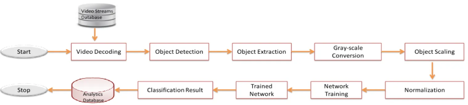
We present the approach of our video analytics system in this section and formulate its mathematical model. The mathematical modeling helped us to tune and train the system and to observe how different hyper-parameters had an effect on the performance of the system which are then visualized and analyzed in the results section. The modeling is performed from the pre-processing stage to final classification which becomes the basis of our scalable and robust video analytics system. Figure 1 shows the workflow of our proposed system.

The proposed system works on decoded video streams and at the very first step it decodes the encoded video frames into individual frames. The number of generated video frames depends on the length of input video stream. 3000 video frames are generated for a video stream of 120 seconds length. The further analysis for object classification is then executed on individual video frames. The

decoded video frames dataset in our system is represented as ; Traininд set X =x1,x2, . . .xn (1)

wherex1,x2, . . .xnrepresents the decoded frames from the video

streams

Each decoded frame of the video stream is converted to gray scale from RGB. This helps to reduce the number of channels from three to one as gray scale video frame consists of only one channel. It reduces the processing time without having an effect on the accuracy of the system.The gray scale converted frames undergo an object detection phase in which a bounding box is created around the area of detection of the desired object i.e. a face in our system. This detection is performed with the help of haar cascade classifier [5]. A labeled frame is denoted by (x; c) where′x′stands for the frame data and ficfi is the ground truth of the object. The associated bounding box after the detection of object is given by;

R(x0,y0xn,yn) (2)

After detection, the detected area is cropped around the area of detection to extract the desired object from the video frame. This narrows down the frame processing area for object classification phase. We denote the extracted object patch by ER(x; b) where x denote the crop of framexiby the bounding boxbi.

The extracted objects from the video frames are scaled at a size of 150*150 pixels and normalized before feeding them into the deep neural network. The normalization is performed to have the pixel values between the range of 0 to 1. The convolutional neural network can perform better with the normalized data. The training setX(capital X) consisting of the extracted objects (ER) from video frames are represented in the normalized form as follows:

X N =f(N(x); N(y))|(x;y)−>D (3) whereX N represents the normalized training dataset obtained by normalizing the frame datax,ybelonging to training data setX. f(.) is the normalization function used to normalize the frame data. The extracted normalized objects are scaled to fixed sizes w * h which are the inputs to convolutional neural network.

The labeled training data used in our system is scarce and in order to enhance it for optimal performance, we executed transfor-mations on the input dataset including translation, skew, rotation flip and different levels of contrast variations. The additional train-ing data by ustrain-ing transformations increases the accuracy of the classifier. These transformations are generated by applying affine displacement fields to video frames. This is achieved by calculating the new location (x,y) with reference to the original location for each pixel of the video frame. For-example if x(x,y)=1, and y(x,y)=0, it shows that the new location of each pixel is shifted to the right by 1. For a displacement field of x(x,y)=αx, and y(x,y)=αy, the video frame will be shifted byα, from the origin point (x,y)=(0,0), whereαcan be any non integer value. LetTbe the set of transfor-mations applied on the training dataset. The training dataset with transformations is represented as;

TX N =TxN1,TxN2, . . .TxNn (4)

The convolutional neural network is then trained to classify and discriminate among the generated classes. The network consists

of multiple alternating layers of convolutional and sub-sampling layers. The convolutional and sub-sampling layers can be given as; Convk,l=д(xk,l∗Wk,l+Bk,l) (5)

Similarly the sub-sampling layer is given as;

Subk,l=д(↓xk,l∗wk,l+bk,l) (6)

Where g(.) represents the activation function which is ’ReLU’ in our system.W andB are the weights and biases of the system. The convolution operation between input and the weights of the network is represented by ’ *’. The sub-sampling layer contains all the inputs in the downsampled form. The activation function of the layers is given as;

h=max(0,a)wherea=W x+b (7) We have added Rectified Linear Units (ReLU) non-linearity in-stead of hyperbolic tangent non-linearity to increase the non-linear properties of the decision function. ReLU works well especially for bigger datasets and trains the network much faster. It ranges from [0,infinity] and models positive real numbers which helps to tackle the vanishing gradient problem. The gradient of max function is given as;

0i f x <0; 1i f x>0 (8) The Local Response Normalization has been adopted to aid gen-eralization and Max pooling is used as the pooling layer in our network. The pooling layer downsamples the feature maps from convolutional layer and reduces the dimensionality as well as the number of parameters to learn. This helps to reduce the overall computational cost. The two response normalization layers follow the first two convolution layers in our proposed system. The three max pooling layers follow the first two local response normalization layers and the last convolution layer. L2 regularization has been introduced to tackle the problem of overfitting which penalizes the network weights and controls them in becoming too large. L2 regularization adds λ2 Õ i θ2 i (9)

where network weights are represented by theta and lambda is the lagrange multiplier.

The weight and bias deltas for the convolutional layers are given as; △Wt,k=LR F Õ i=1 (xi∗Dhi)+m△W(t−1,k) (10) for bias; △Bt,k=LR F Õ i=1 Dh i +m△B(t−1,k) (11)

The weight and bias deltas for the sub-sampling layers are given as;

△Wt,k=LR

F

Õ

i=1

(↓xi∗Dhi)+m△W(t−1,k) (12)

and the bias for sub-sampling layer;

△bt,k=LR F Õ i=1 Dh i +m△b(t−1,k) (13)

The loss function in our case which we try to minimize is given by; L(x)=LR Õ xi−>X Õ xi−>Ti l(i,xiT) (14)

where l(i,xT) is the loss function that we try to minimize during network training. We employed stochastic gradient descent which tries to reduce the loss function during training. It is given by;

Wt+1=Wt−αδL(θt) (15)

Wherewis the weight change with respect to the gradient of the loss function andαis the learning rate. The gradient of the loss function changes rapidly due to the variance present in our training examples after each iteration, so we apply momentum term to keep it smooth and is given by;

Vt+1=ρvt−αδL(θt) (16)

Wt+1=Wt+Vt+1 (17) The convolutional neural network has the softmax layer as the output layer of the network and optimizes negative log likelihood. This can be given as;

l(i,xiT)=M(ei,f(xiT)) (18)

where f(x,T) denotes the function to calculate output values and ’e’ is the basis vector.

4

SYSTEM ARCHITECTURE

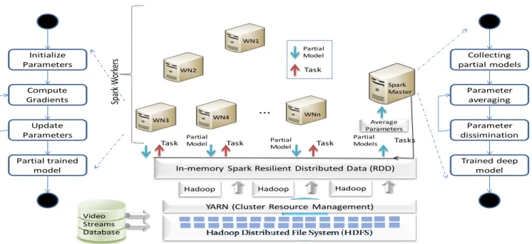
A cloud infrastructure has been proposed to execute the video analysis model proposed in section III. It is compute intensive and works on a larger dataset to perform training of deep model and to classify objects from video streams. We have parallelized the execution of model by using spark which is an in-memory comput-ing framework. The dataset is divided into small subsets which are then passed over to separate neural network models executing on each node of the cluster. Each node trains a partial model and all the partial models from each node are combined through iterative averaging in a central model. This is quite useful in accelerating the execution of deep model on larger datasets. Figure 2 depicts the architecture of our distributed architecture.

The spark master node is responsible to load network config-uration and the initial parameters into the memory. This node is also called as driver node as it drives all the other nodes of the cluster. The network configuration holds the information about the division of data into subsets. Based on the configuration, the data is divided into a number of subsets and is then distributed among worker nodes together with configuration parameters. Each dataset is then used by each work to perform training. Each worker trains a partial model and the averaged results from all the worker nodes are sent back to the master node. The master node holds the fully trained model capable of doing classification on the test data.

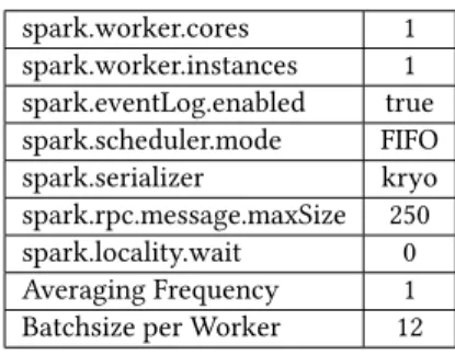
The compute cluster used in our system has one master and eight workers altogether. Each physical slave node is running one spark worker. The dataset comprising of 100GB in size is divided into a number of subsets. The subsets are further divided into mini-batches. The minibatches are exported to disk in the serialized form as the dataset is large and loading it directly into the memory was not feasible. Loading the whole data into memory consumes more memory and increases the split overhead. We have utilized kryo

spark.worker.cores 1 spark.worker.instances 1 spark.eventLog.enabled true spark.scheduler.mode FIFO spark.serializer kryo spark.rpc.message.maxSize 250 spark.locality.wait 0 Averaging Frequency 1 Batchsize per Worker 12

Table 1: Spark Configuration

serialization library to serialize the minibatches. Kryo serialization performs serialization much quicker than java’s own serialization framework and improves performance. Java’s own serialization framework requires high CPU and RAM capacity and is not suit-able for large scale data objects. It is also desirsuit-able to control the rate at which the parameters are averaged and redistributed among the nodes. If the rate of averaging parameters is set to low, this can cause an overhead in initialization as well as network communi-cation. Similarly, if the rate is set to be very high, it can degrade performance as the parameters will deviate extensively. In our case the optimal performance is achieved with a frequency of 16 mini-batches. The minibatches are loaded asynchronously to avoid the delay in loading into the memory. We have configured its value to be 16 as a higher value can result in more use of memory. Table 2 summarizes the tuned parameters for our spark cluster.

An important parameter which is required to be tuned for the training process is to select when data is to be repartitioned. In order to utilize all the resources of the cluster efficiently, it is import to select the number of partitions properly. The values which each partition will hold are also needed to be configured carefully. We have chosen a value of 0.6 based on the experimentations as it ensures the correct number of partitions (balanced partitions). We have not used the default repartition strategy of spark as it does not ensure that each partition is balanced.

The configuration of locality in spark is performed according to the computational demands of the algorithm. As the deep learning algorithm which is being executed on spark has high computation demands, it poses high computation per input minibatch. We have executed one task on each executor; therefore it is much appropriate to transfer the data to a free executor instantly as an executor gets free. It will not be a good setting to wait for a free executor that has local access to the data (default configuration of spark). Transferring the data to a free executor which does not have a local access to data will require the data to be copied across the network, but it allows maximum cluster utilization for our proposed algorithm.

The proposed video analytics system uses iterative mapreduce instead of simple mapreduce framework. Iterative mapreduce frame-work performs multiple passes of mapreduce and is most suitable for convolutional neural network as it is iterative in nature. The proposed system is based on CNN and is highly iterative so the sin-gle pass of mapreduce does not performs quite well. It fully exploits the advantages of iterative mapreduce and performs mapreduce operations in a cascaded way (preceding mapreduce becoming the input to subsequent mapreduce and so on).

Video Streams Database

YARN (Cluster Resource Management) In-memory Spark Resilient Distributed Data (RDD)

Hadoop Hadoop Hadoop

...

Spar

k

W

or

ke

rs

Model Partial_Model

Partial Models Spark Master WN3 Partial Model Task WN2 WN4 WN1 WNn Collecting partial models Parameter averaging Parameter dissimination Trained deep model Initialize Parameters Compute Gradients Update Parameters Partial trained model

Figure 2: Architecture of Distributed Cluster

5

SYSTEM IMPLEMENTATION

The implementation phase consists of pre-processing, training and classification steps. The preprocessing initiates by decoding the video streams into individual frames. The number of generated video frames depends on the length of video stream being decoded. The decoded video frames are converted to gray scale which reduces the number of channels from three to one. The gray scale video frames take much less processing time and edges and contours of an object in a video frame are easily detectable in them. We have used haar cascade classifier to detect objects of interest from the video frames. The video frames are cropped around the area of detection to extract detected objects.

The extracted objects from the video frames are stored in a multidimensional data structure provided by an open-source library named as nd4j. An n-dimensional array (so called tensors) is created to store the pixel values of video frames. We have defined a dataset iterator which has the capability to iterate over the data which is loaded into the memory. The iterator helps to read the data in a vectorized format which is required for the training of the network. The dataset iterator iterates over the dataset objects which contain features as well as the labels for the video frames. Each dataset object contains multiple examples depending upon the configuration. The n-dimensional array created with the help of nd4j library is used to hold the examples along with their labels. A number of minibatches of the dataset have been used in order to tackle the memory requirements problem. As we are working on a large scale video dataset, the volume of data is quiet high and is not practically possible to store whole data at once in the memory. Also, the minibatches of dataset helps to have more updates on the network in one epoch. So we have used a minibatch of 12 in our work. The mini-batch is large and capable enough to represent the input video data and contains all the classes of the objects.

The video frame data is also normalized to have the pixel values between 0 to 1. The normalization of data helps the gradient de-scent optimization approach to converge properly during network training. The gradient descent requires more than one example at a time during the training as more examples will help to create a gradient that encompasses more errors than a single example. A good gradient when using gradient descent approach greatly helps to improve the training, makes the learning consistent and helps to converge on a usable result.

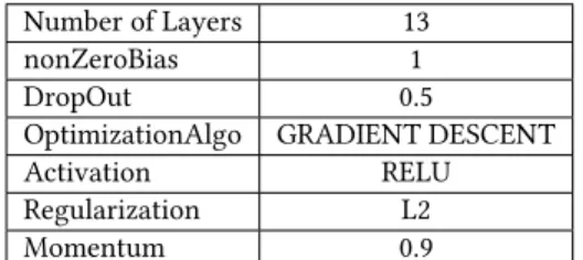
The learning rate is set to be 0.0001. This value is chosen very carefully based on the experimentation. A higher value of learning rate can result in the divergence of the network model away from the error minimum. This will cause the learning process to stop. A small value of the learning rate leads to a slow convergence on an error minimum. The number of epochs and iterations are set to be 5 and 3 respectively. Epoch is the complete pass through our video dataset during the network training. It ensures that the net-work has seen each example present in the dataset once. Iteration on the other hand is a single update of the network parameters. Each epoch during the training phase contains three iterations in our setup. Table II shows the configuration of our deep learning network.

6

EXPERIMENTAL SETUP

This section explains the experimental environment used to develop and evaluate the proposed video analytics system. We have mea-sured and analyzed the training of convolutional neural network by varying hyper-parameters and selected the most appropriate training parameters for the model. The correct classification rate is then measured to evaluate the accuracy of the system. We have

Number of Layers 13 nonZeroBias 1

DropOut 0.5

OptimizationAlgo GRADIENT DESCENT Activation RELU Regularization L2 Momentum 0.9

Table 2: Model Configuration

also measured the scalability of the system by adding various nodes into the cluster.

The architecture of the video analytics system is comprised of cloud resources, infrastructure, and services. The system aims to build a compute cloud with eight cloud nodes. All nodes are based on openstack cloud management stack and are equipped with multi-core CPU processing capacity. These multi-cores are utilized to perform the video analytics operations utilizing Spark computing paradigm. The cloud instances have a ubuntu version of 15.04. Each instance is equipped with 100 GB of secondary storage, 4 VCPUs at a capacity of 2.4 GHz and 16 GB of main memory.

The video dataset used in the proposed system is self generated under controlled environmental conditions. The video streams are by default in the encoded format with H.264 format having an fps of 25, data rate and bit rate of 421 kbps and 461 kbps respectively. These are decoded to generate frames which contain side, front and rear views of individuals. Major challenges such as illumination or blur effects are avoided as they are not the focus of this paper. The total size of decoded video frames used in the experiments varied from 5GB to 100GB.

Apache Spark is used to process the video dataset in a paral-lelized and distributed fashion. The dataset in loaded in the RDDs of spark. Spark spawns a number of executors and each RDD object is accessed by each executor in an iteration to process the job. The iterative MapReduce framework has been used to perform the anal-ysis tasks. Spark executes multiple analanal-ysis tasks in multiple stages and each stage performs further mapping operations respectively. It can also reschedule the tasks in case of task failures.

The video dataset is saved in HDFS which is loaded using spark context and is then converted to INDArrays. The INDArrays are the native tensor representations that are used to pass through the layers of CNN. The first convolutional layer of the network receives and filters the gray-scaled single channeled input video frames with a dimension of 150 x 150 x 1 with a total of 96 kernels. Each kernel has a size of 11 x 11 x 1 and a stride of 4 x 4. The following convolutional layer receives and filters the input with 256 kernels. Each kernel in this layer has a size of 1 x 1 and a stride of 2. The next three convolutional layers are fully connected to each other. Each of these convolutional layers has 384 kernels in it. Each of these convolutional layers constitutes of nonZeroBias. These three convolutional layers are followed by a max-pooling layer with a size of 3 x 3. All these layers are followed by fully connected layers with 4096 neurons. The kernels of the following layers are connected to the kernels of the preceding layers. All the neurons in the fully-connected layers are connected to the neurons of the preceding layer. There are two response normalization layers which

follow the first two convolution layers. There are three max pooling layers which follow the first two local response normalization layers and the last convolution layer. ReLU non-linearity layer follows all the layers of the network.

7

RESULTS AND DISCUSSION

We present and discuss the results of our proposed video analytics system in this section. We measure the performance of the model by following performance characterization: True Positives, False Positives, True Negative, False Negative, Precision, Recall and F1 score.

The value of loss function i.e.L(x)=LRÍ

xi−>X

Í

xi−>Til(i,xiT) at various iterations on the current minibatch is shown in figure 3. It can be seen in the first graph of figure that it goes down after each iteration over time depicting that the learning rate is properly tuned. The learning rate is tuned on the basis of experimentations until the score moves towards the stability. We varied the value of LRto different values including 1e-2, 1e-4 and 1e-6. The effects of these values ofLRonL(x)are plotted in figure 3 and it can be seen that 1e-2 proved to be a good learning rate . The decreasing trend of the graph is also an indication that the training data is normalized properly. L2 normalization scheme with stochastic gradient descent Wt+1=Wt−αδL(θt)is the most appropriate approach for our

net-work training.αis the learning rate which has been varied on the above mentioned valueswis the weight change with respect to the gradient of the loss function. The weights are initialized at random for all the experiments. The selected gradient descent approach does not let the score to increase which normally happens if the learning rate is set too high. The bottom two graphs of figure 3 do not show a proper decreasing trend over multiple iterations. These graphs were produced with aLRof 1e-4 and 1e-6 respectively. It can be seen clearly that the graphs follow a stable state over the iterations and do not show a decreasing trend for learning rate values of 1e-4 and 1e-6. Both the graphs do not fall below 1.0 of the y-axis. The last graph with a learning rate of 1e-6 does not even fall below of 1.5 on the y-axis and is the depiction of bad learning rate, normalization and regularization schemes.

Figure 4 shows the ratio of mean magnitudes of the parame-ters which is the average value of parameparame-ters at various iterations shown along the horizontal axis. It is suggested that the ratio of parameters at various time stamps of iterations should be around -3 on a log10 chart. This is an indicative of a goodLRand appro-priate initialization of other network hyper-parameters. A high divergence of this ratio from the specified value is an indication of unstable parameter initialization and selection. This means that the parameters are unable to learn appropriate features from the training dataset. It can be seen from the first graph of figure that the parameters at various time stamps of iterations are around -3 on the log10 chart. Some parameters started from -2.5 on the y-axis but a convergence towards -3.0 can be easily observed from the figure. Especially 0W tends to converge very rapidly towards -3.0

after some time stamps of iterations.

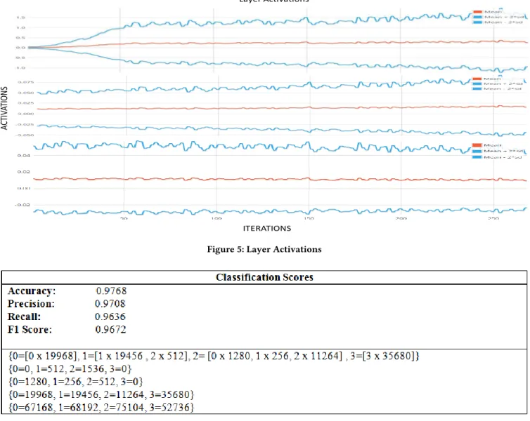
Figure 5 shows the mean magnitudes of the parameter ratios of first convolutional layer used in the network. It can be seen from the layer activations graph that the graph stabilizes after almost 80 iterations which depicts that the network is stable and is not

Model Score vs. Iteration

Figure 3: Model Scores

ITERATIONS PA RA M ET ER RA TIOS

Update: Parameter Ratios (Mean Magnitudes): log

Figure 4: Parameter Ratios

prone to exploding activations problem. The stability of the layer activations graph also shows that the weights of the layers have been initialized correctly with proper regularization scheme. It is observed that the graph stabilizes after few iterations depicting that the model can cope the problem of vanishing or exploding activations. The stability of the graph after some iterations also shows that the weights of the layers have been initialized correctly and proper regularization scheme i.e.λ2Íiθi2is adopted. The value

ofλis varied from 5 * 2 to 5 * 8 but the value of 5 * 1e-4 provided the best results. Please note that this is the ratio for the first convolution layer of the network. It can be seen that the activations at various time stamps of iterations are between the suggested region. This shows that network is in a good learning state from the very first layer with proper learning rate and other network hyper-parameters. The convergence of this ratio as seen from the chart is an indication of stable parameter initialization

Layer Activations ITERATIONS AC TIV AT ION S

Figure 5: Layer Activations

Figure 6: Classification Scores

and selection. On the other hand the bottom two graphs in figure 5 do not show a stability trend.

A normal gaussian distribution is also observed in the histograms of layer parameters. An approximate Gaussian distribution in the histogram of weights for layers shows that the weights have been initialized correctly, updating over each iteration and there is suf-ficient regularization in the network. An approximate Gaussian distribution is also observed in the histogram of layer updates. These updates are the gradients which are generated after applying the regularization, momentum and learning rate. The momentum is given byVt+1=ρvt−αδL(θt)and the value ofρis varied to 0.6,

0.8 and 0.9 for the generated results. The value is finally set to 0.9 in the above graph. Similar to the layer parameters histogram, an approximate Gaussian distribution in the layer updates histogram

represents that the network is not prone to exploding gradient prob-lem. This is mainly because of the usage of gradient normalization which we have added in the network.

After the tuning of the hyper-parameters of the system We have used a test dataset comprising of 88,432 video frames to evaluate the performance of the classifier on the proposed parameters. Figure 6 shows the confusion matrix depicting the overall performance of proposed system. The confusion matrix measures the performance of the system by counting the number of true positives, false posi-tive, true negatives and false negatives. We also calculated various evaluations of the proposed system by using these four counts such as accuracy, recall, precision and F1 score.

The testing dataset consists of video frames from four different individuals. These video frames contain individuals with varying lighting effects and poses. The four different individuals are rep-resented by four different numeric values in the confusion matrix.

It can be seem from the matrix that the classifier performs quite well in distinguishing between different individuals. The individual with label 0 and label 1 has been classified correctly by 19968 and 19456 times respectively. Similarly, the individuals with label 2 and label 3 are classified correctly by 11264 and 35680 times. The system generated an overall quite good accuracy of 0.9768 percent.

Some of the video frames are also misclassified by the system as depicted by the false positives. The video frames labeled as label 1 are classified by classifier as label 3 by the classifier for 128 times. Also, 320 labels which were labeled as label 3 are classified by the classifier as label 0. Label 3 is also classified as label 1 64 times by the classifier. We believe that these frames are misclassified because of the high variance in the pose of the subject. Various lightning conditions also contributed to the false positives of the system. Since the classifier was trained on the dataset which was captured under controlled lightning conditions, therefore various challenges such as blur and illumination effects are not coped by the system. Tackling these challenges is one of the future works of our system. The precision of the proposed system which is the positive pre-diction value is recorded to be 0.9708. The proposed system proved to be precise as well as accurate as depicted in the confusion matrix. The recall and F1 score of the system are recorded to be 0.9636 and 0.9672 respectively. Recall can also be referred to as the sensitivity of the system while F1 depicts the overall performance of the sys-tem with 0.0 to be the worst score and 1.0 being the best score of the system. Precision and F1 scores for the system are calculated as;

F1=2T P/(2T P+FP+F N) (19) Recall =T P/(T P+F N) (20)

Execution on Cloud Infrastructure:

The proposed system is executed on the cloud infrastructure as described in the experimental setup section. The input data is first loaded in the RDDs of spark. Spark launches a number of executors and the RDD objects are accessed by each executor in an iteration. The cache manager is responsible to handle the results of the iterations. It maintains a memory pool and retains the iteration results in it. In case the data is not applicable anymore, it is not needed to be retained in the memory and can be saved on the disk. In this way spark manages the data and keeps a part of data in memory and the rest of the data is stored on the disk.

We have used the iterative MapReduce framework to perform the analysis of the video streams. Each node in the cloud can execute one or more than one analysis task on the input dataset. In iterative reduce, an analysis task comprises of multiple map and reduce tasks. These multiple map and reduce tasks perform the classification of objects from the input dataset. Spark executes these task in multiple stages and each stage performs further mapping operations. The iterative MapReduce framework is also responsible to schedule the map and reduce tasks and also rescheduling of tasks in case of task failure.

The total size of decoded video frames used in the experiments varied from 5GB to 100GB. These large set of individual frames data is not suitable to be directly fed into the spark cluster with

0.36 0.68 1.13 1.63 2.18 0.3 0.57 1.05 1.43 2.1 20 40 60 80 100 Da ta Tra nsfer Time (H ours) DataSet Size (GB)

Data Transfer Time to Cloud Storage

128 MB 256 MB Expon. (256 MB)

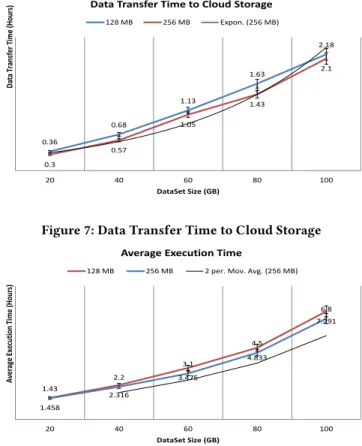
Figure 7: Data Transfer Time to Cloud Storage

1.458 2.316 3.475 4.833 7.291 1.43 2.2 3.1 4.5 6.8 20 40 60 80 100 Avera ge Execution Time (H ours ) DataSet Size (GB)

Average Execution Time

128 MB 256 MB 2 per. Mov. Avg. (256 MB)

Figure 8: Average Execution Time

iterative reduce framework. The individual video frames are small in size and iterative reduce is designed to work on large data files. Processing of smaller files with iterative reduce only results in the loss of overall performance of the system. We have bundled the individual frames by using a batch process and then transferred it to compute cloud for processing. The time required to bundle the data varies with the amount of video frames being considered. This time is directly dependent to the size of the dataset. For a dataset of 10GB to 100GB, the time of batch process varied from 0.25 hours to 3.8 hours. Addition of more video frames in the dataset increases the time as well. However, this process needs to be executed only once and the resultant data can be retained in the cloud storage for future analysis.

The data is needed to be transferred to cloud data storage to perform analysis tasks on it. The transfer time to cloud data storage depends on a number of factors such as; network bandwidth and cloud data storage block size. This time is also dependent on the size of the data being transferred. To have an estimate of the transfer time, we measured the transfer time for various sizes of data and plotted in Figure 7. It can be observed from the figure that the transfer time varied from 0.36 to 2.18 for a dataset size of 20GB to 100GB. We have also measured this time by changing the cloud storage block size from 128 MB which is the default size to 256MB. However, very little improvement has been recorded in the transfer time by varying the block size.

We have performed the training on multiple nodes of cloud and measured the scalability and robustness of the proposed system. To have a good estimate of the training time we have executed multiple tests on multiple sizes of datasets and plotted their average execution time in Figure 8. The average execution time gives a measure of how much training time on average is required to train the proposed system on a specific size of dataset. The dataset sizes have been varied from 20GB to 100GB to measure the time on various cloud nodes. It has been observed that the execution time increases by increasing the size of dataset.

The same set of experiments is then repeated by changing the block size. The change in the block size causes a change in the num-ber of partitions of the dataset. So the experiments were repeated with different block size to see if there are any improvements in the execution time of the system. It can be seen from the figure that the execution time varied from 1.45 hours to 7.29 hours for a block size of 128MB. For the block size of 256MB, the execution time showed a very little improvement from 1.43 hours to 6.8 hours for the same size of dataset. So the variation in block sizes has a minor impact on the execution time of the system.

8

CONCLUSION AND FUTURE WORK

A cloud based video analytics system has been presented and eval-uated in this paper. The system works in three stages and employs deep learning algorithm to classify objects from video streams. It can enhance its own training data by performing various transfor-mations including rotation, flip and skew on the input dataset. The system learns features from large amounts of input data by per-forming training in parallel on a multi-node in-memory cluster. The execution time varied from 1.45 hours to 7.29 hours for the dataset size ranging from 20GB to 100GB on the cloud. The efficient tuning of the hyper-parameters of the system through mathematical model makes it highly accurate and robust to classification errors. The validation of the system is performed by an object classification case-study and extensive experimentation revealed an accuracy and precision of 0.97 and 0.96 respectively. Several factors contributed to achieve high accuracy such as optimal selection of learning rate, regularization, normalization and optimization algorithms. The de-sign of multi-layer network including number of layers and their parameters also played a major role in achieving high accuracy in the system.

In future, we would like to leverage reinforcement learning based models to improve the performance of our video analytics system. This will also help to extend the functionality of the system by clas-sifying other objects such as vehicles or pedestrians. The develop-ment of an automated mechanism for hyperparameter optimization of deep learning models will also be the part of our future work. We would also like to deploy the proposed system on an in-memory processing cloud coupled with the computation power of GPUs to improve performance and training time. More innovation will be added on the infrastructure side by incorporating memory models to enhance the scalability and throughput of our video analytics system.

REFERENCES

[1] DÃľniz, O., Bueno, G., Salido, J. and De la Torre, F., 2011. Face recognition using histograms of oriented gradients. Pattern Recognition Letters, 32(12), pp.1598-1603.

[2] Abdel-Hakim, A.E. and Farag, A.A., 2006. CSIFT: A SIFT descriptor with color invariant characteristics. In Computer Vision and Pattern Recognition, 2006 IEEE Computer Society Conference on (Vol. 2, pp. 1978-1983). IEEE.

[3] Yaseen, M.U., Zafar, M.S., Anjum, A. and Hill, R., 2016, March. High performance video processing in cloud data centres. In Service-Oriented System Engineering (SOSE), 2016 IEEE Symposium on (pp. 152-161). IEEE.

[4] Yaseen, M.U., Anjum, A. and Antonopoulos, N., 2016, December. Spatial frequency based video stream analysis for object classification and recognition in clouds. In Proceedings of the 3rd IEEE/ACM International Conference on Big Data Computing, Applications and Technologies (pp. 18-26). ACM.

[5] Yaseen, M.U., Anjum, A., Rana, O. and Hill, R., 2017. Cloud-based scalable ob-ject detection and classification in video streams. Future Generation Computer Systems.

[6] Karpathy, A., Toderici, G., Shetty, S., Leung, T., Sukthankar, R. and Fei-Fei, L., 2014. Large-scale video classification with convolutional neural networks. In Proceedings of the IEEE conference on Computer Vision and Pattern Recognition (pp. 1725-1732).

[7] Krizhevsky, A., Sutskever, I. and Hinton, G.E., 2012. Imagenet classification with deep convolutional neural networks. In Advances in neural information process-ing systems (pp. 1097-1105).

[8] Yue-Hei Ng, J., Hausknecht, M., Vijayanarasimhan, S., Vinyals, O., Monga, R. and Toderici, G., 2015. Beyond short snippets: Deep networks for video classification. In Proceedings of the IEEE conference on computer vision and pattern recognition (pp. 4694-4702).

[9] Simonyan, K. and Zisserman, A., 2014. Two-stream convolutional networks for action recognition in videos. In Advances in neural information processing systems (pp. 568-576).

[10] Deng, J., Dong, W., Socher, R., Li, L.J., Li, K. and Fei-Fei, L., 2009, June. Ima-genet: A large-scale hierarchical image database. In Computer Vision and Pattern Recognition, 2009. CVPR 2009. IEEE Conference on (pp. 248-255). IEEE. [11] Levi, G. and Hassner, T., 2015. Age and gender classification using convolutional

neural networks. In Proceedings of the IEEE Conference on Computer Vision and Pattern Recognition Workshops (pp. 34-42).

[12] Ciregan, D., Meier, U. and Schmidhuber, J., 2012, June. Multi-column deep neural networks for image classification. In Computer Vision and Pattern Recognition (CVPR), 2012 IEEE Conference on (pp. 3642-3649). IEEE.

[13] LeCun, Y., Cortes, C. and Burges, C.J., 2010. MNIST handwritten digit database. [14] Krizhevsky, A., Nair, V. and Hinton, G., 2014. The CIFAR-10 dataset. online:

http://www. cs. toronto. edu/kriz/cifar. html.

[15] Huang, F.J. and LeCun, Y., 2006, June. Large-scale learning with svm and con-volutional for generic object categorization. In Computer Vision and Pattern Recognition, 2006 IEEE Computer Society Conference on (Vol. 1, pp. 284-291). IEEE.

[16] Taigman, Y., Yang, M., Ranzato, M.A. and Wolf, L., 2014. Deepface: Closing the gap to human-level performance in face verification. In Proceedings of the IEEE conference on computer vision and pattern recognition (pp. 1701-1708). [17] Huang, G.B., Ramesh, M., Berg, T. and Learned-Miller, E., 2007. Labeled faces in

the wild: A database for studying face recognition in unconstrained environments (Vol. 1, No. 2, p. 3). Technical Report 07-49, University of Massachusetts, Amherst. [18] Kang, K. and Wang, X., 2014. Fully convolutional neural networks for crowd

segmentation. arXiv preprint arXiv:1411.4464.

[19] Kang, K., Ouyang, W., Li, H. and Wang, X., 2016. Object detection from video tubelets with convolutional neural networks. In Proceedings of the IEEE Confer-ence on Computer Vision and Pattern Recognition (pp. 817-825).

[20] Zha, S., Luisier, F., Andrews, W., Srivastava, N. and Salakhutdinov, R., 2015. Exploiting image-trained cnn architectures for unconstrained video classification. arXiv preprint arXiv:1503.04144.

[21] Pfister, T., Simonyan, K., Charles, J. and Zisserman, A., 2014, November. Deep convolutional neural networks for efficient pose estimation in gesture videos. In Asian Conference on Computer Vision (pp. 538-552). Springer, Cham. [22] A. R. Zamani and M. Zou and J. Diaz-Montes and I. Petri and O. Rana and A.

Anjum and M. Parashar, 2017, Deadline Constrained Video Analysis via In-Transit Computational Environments, IEEE Transactions on Services Computing. [23] Anjum, A., McClatchey, R., Ali, A. and Willers, I., 2006. Bulk scheduling with the

DIANA scheduler. IEEE Transactions on Nuclear Science.

[24] Anjum, A., Abdullah, T., Tariq, M., Baltaci, Y. and Antonopoulos, N., 2016. Video stream analysis in clouds: An object detection and classification framework for high performance video analytics. IEEE Transactions on Cloud Computing.