Home Activity Pattern Estimation Using Aggregated Electricity Consumption Data

*_{Corresponding author: e-mail: [email protected]} **_{Corresponding author: e-mail: [email protected]} https://doi.org/10.18494/SAM.2021.2992

ISSN 0914-4935 © MYU K.K. https://myukk.org/

Home Activity Pattern Estimation

Using Aggregated Electricity Consumption Data

Kotaro Ishizu,

Teruhiro Mizumoto,

Hirozumi Yamaguchi, and Teruo Higashino

Graduate School of Information Science and Technology, Osaka University, 1-5 Yamadaoka, Suita, Osaka 565-0871, Japan

(Received July 27, 2020; accepted September 23, 2020)

Keywords: activity recognition, machine learning, power consumption data, model selection

In this paper, we propose a low-cost, noninvasive home activity recognition method using low-resolution power consumption data. Notably, we tackle the following two challenges. Firstly, we use only the time series of power consumption data aggregated per house and measured approximately every 20 s, which is usually used for demand monitoring by smart meters. We design a set of activities that can be recognized using such low-resolution data and find an appropriate feature set to train and test the balanced random forest classifier. Secondly, we consider the divergence of activity patterns seen in different households. Since supervised learning dedicated to each household is not a realistic solution, we arrange different classifiers trained with different household data in supervised learning and present a method of automatically choosing the best-fit classifier for an unseen household in the online phase. We evaluated our method with an aggregated power consumption dataset collected from eight real homes over 191 days. We confirmed that our method achieved a recognition accuracy of 70% for activities using such a low-resolution aggregated power consumption dataset, and that our proposed fitness scores were effective for choosing the best classifiers.

1. Introduction

In recent years, with the remarkable development in the field of sensing technology, we have been able to recognize human activities easily from sensor information. Hence, the demand for various services based on activity recognition has increased. In particular, new services such as home energy optimization, health advice, and home healthcare based on an awareness of behavior in homes have attracted much attention.

The Statistics Bureau of Japan has reported that 16% of Japanese elderly people live alone.(1) Elderly people living alone have less social involvement. Therefore, they have a high risk of dying alone. This problem, called kodokushi in Japanese, is one of the pressing social issues in Japan’s aging society. The health of young single persons should also be considered and cared for. Physical and mental problems may lead to disturbances in life patterns and a decrease in the number of outdoor activities. Home activity monitoring plays an important role in preventing such situations by sharing the daily living status of vulnerable people with families, caregivers,

and counselors. Developing human-friendly, low-cost technologies for recognizing and understanding home activities is a common goal.

Many activity recognition technologies with various sensor devices have been proposed thus far. Vision-based activity recognition methods such as that in Ref. 1 can achieve the highest accuracy using the current technology, but most people are unwilling to install cameras in their homes owing to privacy concerns. Methods such as that in Ref. 2 require residents to wear and charge wearable devices at home; such methods are also invasive and impose extra effort on most people. They may also result in a lack of sensing data for certain periods during which the residents do not want to wear them.

To address such issues, low-invasivity and low-resolution sensors have been used in different ways. Chen et al.(3) _{present a real-time activity recognition method of comprehensively using} sensing information gathered via a number of different sensors installed in a smart house. Furthermore, Zhang et al.(4) _{proposed a method of recognizing home activities by detecting the} use of home appliances via power consumption monitors installed to each appliance in a home. The methods in these studies use low-cost sensing technologies, but they also have a certain cost and require maintenance services such as installation, calibration, power supply, and location management.

In this paper, we propose a low-cost, noninvasive home activity recognition method using low-resolution power consumption data to tackle the following two challenges. Firstly, we focus on a time series of power consumption data aggregated per house and measured approximately every 30 s, which is usually used for demand monitoring by smart meters. The existing methods that use a watt monitor attached to each power outlet can analyze the waveform of power consumption of the appliance and identify it for activity recognition. The challenge in our method is that the aggregated power consumption data are a time series of the power consumption of a mixture of home appliances as well as built-in home facilities. We choose a set of activities, sleeping, cooking, going out, and others, that can be recognized from such low-resolution data and find an appropriate feature set to train a balanced random forest classifier. Secondly, we consider the divergence of activity patterns seen in different households. Since supervised learning dedicated to each household is not a realistic solution, we arrange different classifiers trained using different household data in an offline phase and choose the classifier that best fits with an unseen household in an online phase. More specifically, we collect long-term activity-power data from multiple real homes and train a balanced random forest classifier for each home in the offline phase. In the online phase, using a metric called classifier fitness, which returns the fitness score of each classifier to the measured aggregated power consumption, the best-fit classifier is chosen. Consequently, the presented approach enables the possibility of home activity recognition without the need for sensors, even though the activities detected are limited to basic ones. It also copes with the issue of activity pattern divergence of individual households by introducing a simple metric to assess the fitness of the model to the measured power consumption data.

We conducted a long-term experiment where aggregated power consumption data of 30 s intervals were gathered in eight real homes over 191 days to evaluate the approach. We annotated the activities to the dataset referring to the obtained household profiles (e.g., home

appliances owned, built-in home facilities, and usual bedtime) and the data from human detection sensors installed for this annotation purpose only.

We conducted experiments to evaluate the accuracy of activity recognition and classifier selection using these data. Firstly, we evaluated the proposed fitness score to choose the best-fit classifier. For comparison, we introduced five different best-fitness scores and evaluated the correlations between the value of each score and the F-measure of the model. The proposed

score achieved the highest correlation (−0.84) with F-measures of the models, which means

that it is able to choose the best classifier. Furthermore, we confirmed that our proposed home activity recognition method using the fitness score achieved a recognition accuracy of 70% for activities such as cooking, sleeping, and going out, which are effective for noninvasive remote monitoring.

2. Related Work

Various types of activity recognition method to assist residents in their homes have been proposed thus far. The majority of methods recognize activities of daily living in the home through machine learning using various types of sensor device. In this section, we survey and classify the existing camera/microphone-based, wearable-device-based, and low-cost-sensor-based methods.

2.1 Camera-microphone-based approaches

Camera-based activity recognition is the most intuitive approach and is able to recognize activities with high accuracy. Li and Hua(1) proposed a method of recognizing six activities related to human motion by template matching to each video frame. It achieved a recognition accuracy of approximately 93 to 100%. Rostamzadeh et al.(5) proposed a method of recognizing 10 types of activity using local motion and body pose with a recognition accuracy of approximately 98%. Nakahara et al.(6) proposed a method of recognizing eight activities on the basis of the motion of human joints observed using a laser-based time-of-flight camera. Ouchi and Doi(7) proposed an indoor-outdoor activity recognition method in which the accelerometers and microphones of smartphones are used. They achieved the classification of seven activities in daily living (ADLs) every second with an accuracy of 85% on average. Brdiczka et al.(8) proposed a method of using an ambient sound sensor and a 3D video tracking sensor, and achieved a recognition accuracy of 70 to 90%.

The above methods can achieve high recognition accuracy. However, they require people to accept being in a continuously monitored environment where privacy-sensitive data are collected. Therefore, the applicability is limited if we target activity recognition in individual homes.

2.2 Wearable-device-based approaches

Recent downsizing technologies for sensors, displays, and batteries have enabled smaller but more functional wearable devices such as smartwatches. These wearable devices continuously

collect human activity and vital data. Hence, activity recognition using sensors of wearable devices is a reasonable way to track the status of humans. Lee and Mase(2) proposed an activity recognition method of using two wearable sensor devices attached to the leg and waist as pioneers of these types of technique. As a more practical method, Kalantarian et al.(9) proposed a method of monitoring eating habits using a necklace embedded with a piezoelectric sensor. Similarly, Maekawa et al.(10) focused on the magnetic field generated by home appliances when used and proposed a method of recognizing ADLs related to the usage of appliances.

Despite their high-accuracy monitoring of humans, including vital signs, one disadvantage of using wearable devices for home activity recognition is that residents are required to always wear the devices. Another issue is the need to charge the device periodically. Residents may also often take off or forget to wear devices, which leads to a lack of data in particular time slots. 2.3 Low-cost sensor-based approaches

Considering the above problems, methods in which noninvasive and low-cost sensor devices are installed have attracted much attention. Van Kasteren et al.(11) proposed a method of recognizing 10 types of activity, such as “eating” and “watching TV”, in which door sensors, pressure-sensitive mats, floating sensors, and temperature sensors are used with a recognition accuracy of 49 to 98%.

Furthermore, Chen et al.(12) and Fleury et al.(13) proposed methods of recognizing complex living activities such as “making coffee” and “cooking pasta” using various sensors including contact, motion, tilt, and pressure sensors. However, these methods require multiple heterogeneous sensors, which incur installation and maintenance costs, as discussed earlier. Power-monitoring devices are also widely used for activity recognition. Rollins and Banerjee(14) proposed a method of recognizing activities using power consumption data by linking the operation of home appliances to the amount of power consumption. Methods of recognizing 10 types of ADL from the time-series data of the residents’ positions and power consumption of home appliances have been proposed.(15,16) Nevertheless, hardware installation and maintenance are still necessary for the power monitoring of each appliance. Although state-of-the-art smart houses can monitor the power consumption for each outlet separately, such houses are not yet popular in many regions and countries.

It is worth noting that there are known approaches called nonintrusive load monitoring (NILM) to estimate operating conditions and behaviors of home appliances from aggregated power consumption data. After these operations of appliances are known, they can be used for activity recognition. However, these approaches are totally different from ours in the following points. Firstly, most of them require dedicated devices that can measure the data with high frequency [i.e., sampling rate of 50–100 MHz(17,18)_{]. Secondly, they need a dedicated model for each appliance} or house. Lee et al.(19) proposed a method of recognizing seven types of activity using low-rate aggregated power consumption data (0.2 Hz). However, they make two assumptions, of which the appliances in an environment have been informed and the states of these appliances are predefined. Somchai et al.(20) _{proposed a method of recognizing the behavior of air conditioning} units and refrigerators using low-rate aggregated power consumption data (1 Hz). Chalmers

et al.(21) _{proposed a method of detecting dementia using the low-rate aggregated power} consumption data (0.1 Hz) of the operation of five types of home appliance. However, a support vector machine/random forest (SVM/RF)-based model trained on activity data from the target household is needed. In other words, a sufficient amount of activity data must be obtained to train the model for each home; however, this is not practical. An estimation model must be built for each home appliance, which is often unsuitable for building general home activity recognition systems, owing to the wide variety of appliance products and home built-in electric facilities on the market and in the home, as well as the diversity of activity patterns.

There is also a service that estimates the electricity consumption of home appliances from the data collected from smart meters.(22) This service monitors electricity consumption over a long period of time, calculates the ratio of the amount of electricity consumed by each household appliance to the monthly amount consumed, and gives advice on energy saving. Unfortunately, it does not provide a methodology for recognizing activities.

2.4 Our contributions

To the best of our knowledge, only a few research groups(17,19,21) _{have tried to estimate the} operations of home appliances (not human activities) using the aggregated power consumption measured by power switchboards/meters. However, a dedicated, noncommercial device that can measure the data with high frequency (i.e., sampling rate of 100 MHz) was required in Ref. 17, and in Ref. 19, it was necessary to build an estimation model for each home appliance using precollected data. This is unrealistic owing to the variety of appliances and home built-in electric facilities.

Although obtaining aggregated power consumption data using smart meters with a low sampling rate (1 sample per 20 s in our case) is noninvasive and needs no extra investment for data acquisition, there is a challenge in utilizing such data for services such as activity recognition as the data are temporally and spatially coarse grained. Ongoing research has enabled behavioral estimation using models tailored to each household. However, it again is unrealistic to obtain behavioral data to build such models. From this perspective, ours is the first work on tackling this challenging problem of realizing noninvasive, zero-device-cost activity recognition using only low-rate aggregated power consumption data without house-dependent classifiers.

3. Methodology Overview

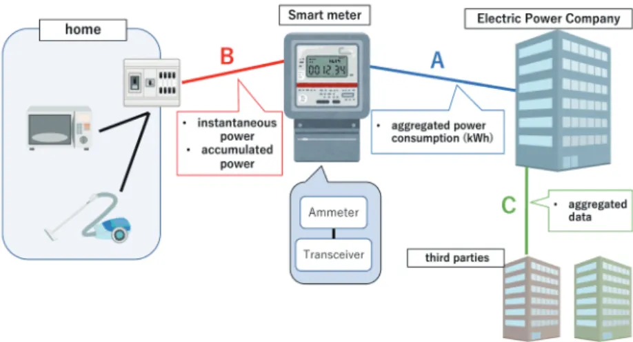
Figure 1 shows our system for aggregate power consumption (APC) data acquisition. We assume that a smart meter has been installed in each home by an electric company. The Japanese government is now promoting the introduction of smart meters into homes(23) and electric companies have already started deploying them. A typical smart meter system in Japan defines three connections, called routes A, B, and C, among the customer, the electric company,

and the smart meter. Route B is used to gather data from the home by the smart meter, and the smart meter can request the power utilization data, such as instantaneous power and accumulated power, at any time. Hereafter, we define the total power consumption of one home during the time period T as the APC, where T = 20 (s) in our dataset. In the proposed method, we assume that APC data of homes are available, and we utilize this information to provide value-added services. In particular, we leverage these data for daily activity monitoring without additional cost, in collaboration with one of the largest electricity companies in the Osaka area, whose aim is to provide a low-cost, remote, and noninvasive monitoring system for people (e.g., elderly persons and students) living alone.

3.2 How it works

Our activity recognition method focuses on three typical activities at home, sleeping, going out, and cooking, which are included in the ADLs defined in Ref. 24. We also assume a category called others that includes all the other activities that do not fall into any of these three ADLs. For activity recognition using APC data, we consider the following insights obtained from our preliminary experiments and data observations.

(1) Home appliances such as TVs and microwave ovens are directly switched on and off by residents. Therefore, if their power consumption appears in the APC, we can conclude that there is some human activity.

(2) Always-on home appliances such as refrigerators have low relevance to home activities. (3) Built-in facilities such as electricity-operated boilers, lights, and electric toilet seats (very

popular in Japan) need to operate continuously. Therefore, they also have low relevance to home activities.

Our method is designed for services, such as an elderly monitoring service, that use the activities of target persons. Also, changes of the life patterns, such as a decrease in sleep time, fewer meals, and the reduction in the number of outside activities, are signs of mental disease.(25,26) Considering those facts, we discussed, with a company that plans to launch a new monitoring

service utilizing APC data, the significant activities that must be recognized to run the service. As a result, we concluded that sleeping, going out, cooking, and others are the fundamental and useful ADLs for achieving the goal.

Straightforwardly, for activity recognition from the APC, we need to eliminate the effects of appliances and facilities associated with (2) and (3) to identify those associated with (1).

Promising activities for recognition include sleeping at night and going out, mostly in the daytime. On the other hand, it is not reasonable to assume such a temporal similarity for more individual-dependent activities such as cleaning and cooking.

Our recognition algorithm works as follows. A given time series of APC data, which is gathered every t s (t = 20 in our dataset), is divided into T min time window data.

If T is short, we may not be able to extract sufficient features for recognition. In particular, the number of peaks, which is one of the primary factors characterizing the window, may decrease, and this will affect the estimation accuracy. Furthermore, if T is long, for example, T = 60, multiple activities may take place in a single window, which will confuse the classifier. Therefore, we consulted with several companies that have been considering the operation of a monitoring service and concluded that an interval of 30 min (T = 30) is the appropriate granularity for activity recognition.

Then, for each time window, we estimate the most probable activity in the time slot by supervised learning that captures the characteristics of power consumption patterns. The challenge here is how to build a house-dependent model for estimation, but it is not reasonable to conduct supervised learning for each home considering the difficulty in acquiring the ground truth. Transfer learning is a promising approach to facilitating domain-specific learning from a smaller amount of data. However, in our case, obtaining the ground-truth data itself is impossible as users must be asked to record their activities before starting the service. In order to achieve our goal, we leverage our dataset to arrange several models that fit different types of lifestyles and develop a model selection metric that enables us to choose the model that best fits the APC data of the target house. The details are explained in the following section.

4. Activity Recognition Algorithm

As we mentioned in the previous section, we divide the given APC data into a series of window data of length T (min) and extract the features in each window. Then, we give one of the four activity labels, namely, going out, sleeping, cooking, and others, to each time window and use it to train multiclass classifiers. Note that the average sleeping time per day is 7.5 h in Japan, which is about 30% of a person’s lifetime. This means that data with the “sleeping” label are much more common than those with “cooking”, which usually accounts for, at most, 2 h per day, or even those with “going out”. Therefore, we employ a Balanced Random Forest (BRF)(27) as the model of classifiers; this is an enhanced version of a random forest and can address imbalanced data. It can balance the samples when creating subsets of samples for making decision trees.

In order to investigate how the power consumption by typical home appliances appears in the APC, a preliminary experiment was conducted in a real home for 25 days of the period between December 26, 2018 and January 25, 2019. We measured the power consumption of a washing machine, a TV, a microwave oven, a humidifier, a dryer, a gas stove (electrically controlled), and an oven toaster individually with 30 s intervals using commercial watt monitors and obtained APC data as a simple mixture of their power consumptions.

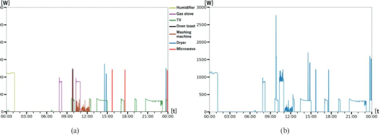
Figure 2 shows examples of the power consumption of individual appliances’ and APC data. In the individual power consumptions, we observed clear peaks of power consumption for the cooking appliances (oven toaster and microwave oven) and the dryer at the start and end of their use. On the other hand, the gas stove and humidifier were operated for a long time while consuming a certain amount of power (about 800 W). We found that the TV and washing machine were also operated for relatively long times, although the time variation of power consumption was larger than that of most of the other devices.

Even though this preliminary experiment was carried out in an ideal, controlled environment without noise from built-in facilities and unknown appliances, we found it very difficult to fully identify the operation of appliances. However, we obtained the following insights by analyzing the data. Firstly, if the operation of home appliances is not observed in a time window, the resident is probably in the state of sleeping, going out, or others, which are activities unrelated to home appliances. Secondly, compared with the minimal APC value throughout the day, if the observed APC value is sufficiently high, some home appliances such as air conditioners may be operating during the time window and the probability of going out is low. Furthermore, going out and sleeping can be roughly distinguished by considering their timeframes. Cooking appliances such as microwaves, oven toasters, and induction cookers tend to consume more power as they need heating. On the other hand, as seen in the preliminary experiment, the power consumption of the washing machine is variable, which may be reflected in the variance of APC data. Moreover, the activity and APC in previous time windows may have correlations with the activity in the current time window.

Fig. 2. (Color online) Power consumption data in preliminary experiment (controlled environment). (a) Power consumption by individual appliances. (b) APC.

Therefore, these should also be considered as feature quantities. On the basis of the above discussion and insights, for each time window, we use the following as features: the number of peaks; the peak average; the difference between the values of two consecutive APC samples; the minimal, maximal, average, and standard deviation of APC values; and the power spectrum obtained by a fast Fourier transform (FFT). In addition, the minimal, maximal, and standard deviation of APCs in the last six time windows and the activity in the last window are also used as features for training the classifiers. A peak is generated by a continuous fluctuation with upward and downward trends. In this method, the number of peaks in one window is used as a feature. The use of home appliances such as washing machines and TVs, which have internal controls and operate for long periods, increases the number of peaks in the power supply. Therefore, it is possible to recognize their operations using the peak-number feature. Moreover, the power spectrum uses the FFT to divide the original time series data into 30 different periods of 1 to 30 min, and the magnitude of each frequency component is used as a feature. The idea behind using frequency decomposition is that cooking home appliances such as microwave ovens often consume a large amount of energy in a short time, and this feature appears in the high-frequency components. On the other hand, appliances with long operation time, such as a TV, may affect the low-frequency component. The total number of features is 133. Note that the activity in the last window is not available in the classification phase. Therefore, we use the predicted activity as the feature.

4.2 Classifier selection technique

Because of the coarse-grained granularity of APC data and individual-dependent features, the selected feature quantities may not exactly represent the activities. This problem may be resolved if we can build a classifier for each house. Nevertheless, this is not realistic as we need to collect ground-truth data from each home to train the classifier.

Transfer learning(28) _{uses an existing classifier as a way of obtaining a domain-specific} classifier tailored to the estimation target. However, even with such a promising technique, the training data of the target home are still required, which is a barrier to plactical deployment. To solve this problem, we take an approach of building multiple classifiers that correspond to different types of homes. Then, we provide a novel metric that represents classifier fitness to choose the classifier that best fits the unseen target home in order to estimate activities. The fitness score of each classifier to a target home is defined as a function of the training dataset for that classifier and the obtained test dataset. Figure 3 shows the calculation procedure for the fitness score. Let us assume that there are N homes denoted as 1, 2, ... and N. Firstly, in an offline phase, we train a classifier, denoted as fi, for home i using training data from home i (denoted as TRi). TRi consists of power consumption data and corresponding activity labels. In an online phase, test data from a new home z (z ∉[1, ]N ) are given to all N classifiers, f1, ..., fN, for activity recognition. The set of predicted activities from each home i (fi(z)) is fed into the fitness score function (denoted as scorei) with the training data TRi. scorei calculates the similarity between fi(z) and TRi, and returns the fitness score of these two datasets. Finally, fi(z) with the highest fitness score among the classifiers is chosen as the final estimation result. Note that we may use a subset of TRi as input to the function scorei for computational efficiency.

In this study, we design six fitness score functions. Their selection capabilities will be tested in the performance evaluation section. These functions respectively calculate the sleeping score, going out score, sleeping and going out (s–g) score, dynamic time warping score (DTW_score), mode DTW_score, and ratio score.

The concept of having the sleeping, going out, and s–g scores is based on the hypothesis that the training data labels (ground truth activities) and those estimated from the given test data have correlations in terms of their appearance time in each day. Therefore, these scores become higher if more time windows have the same activity labels between the ground truth and the estimation, and we look at the appearance time similarity of sleeping, going out, and both sleeping and going out. The DTW_score and mode_DTW_score are based on a different hypothesis that the ground truth and estimation have correlations in terms of daily appearance patterns in each day.

Finally, the ratio score is based on a hypothesis that the ground truth and estimation have correlations in terms of the ratio of activity appearance.

Table 1 shows a summary of these six fitness scores. The first hypothesis is based on observations that sleeping or going out or both do not differ among homes.

As an input to scorei, we use a set of daily sequences of true and predicted activity labels, where each sequence consists of 48 labels (with the time window length T of 30 min). In this process, the sleeping activities that last less than 3 h or longer than 15 h, and the going out activities longer than 15 h are excluded as anomalous cases. Then, samples of L days of data are randomly chosen from each set of training data TRi. Equations (1)–(3) define the sleeping, going out, and s–g scores, respectively. We note that pred is a binary function with a value of 1 if the augment predicate is true, and 0 otherwise. TRi(u, t) and fi(z)(u, t) return the activity labels of the t-th time window of the u-th day in TRi and fi(z) (i.e., the true and predicted activity labels), respectively.

1,..., 1,..., 1,...,48 1 _ ( ) ( ( , ) ( )( , ) ) 48 i i i u L v K t

sleeping s z pred TR u t z v t sleep ngi

L K f core = = = = = = ⋅ ⋅

∑ ∑ ∑

goingout score z pred TR u t f z v t goout

L K = = = = = = ⋅ ⋅

∑ ∑ ∑

s g sc e z pred TR u t z v t sleep ng or goouti

L K

or f

= = =

− = = =

⋅ ⋅

∑ ∑ ∑

To test the second hypothesis (appearance pattern similarity), we introduce two DTW-based scores, DTW_scorei and mDTW_scorei.

DTW is a method of determining the similarity between two waveforms. DTW can determine the similarity of the overall shape even if the period and time are different. On the other hand electricity consumption data often expand or contract nonlinearly, because the time of day and the amount of time people spend at lunch every day often change by 30 min to 1 h. Therefore, we used DTW to calculate the similarity of behaviors that appear in the power waveform.

In both cases, we use two model parameters, Q and W. W is a penalty parameter for the insertion or deletion of an activity label into or from the daily sequence of activities, and Q is that for the replacement of an activity label with another in the sequence. DTW_scorei is defined as the average minimal edit distance (DTW distance), denoted as DTWQ,W(s1, s2), between the two daily sequences s1 and s2 of activity labels. Moreover, we define a variant of this DTW score, mDTW_scorei (called mode DTW_score). This score function picks the most frequent activity in each time windows. The sequence of the such activities during M days is called representative daily sequence.

We let seqi(u) denote the u-th day’s sequence of activity labels and MAX_DTWQ,W be the maximal DTW distance.

Then, DTW_scorei is defined as

DTW_scorei , 1,..., 1,..., , 1 _ ( ( ), ( )) _ i Q W i i u L v K Q W

DTW scor DTW seq u seq v

L K MAX D W e T = = = ⋅ ⋅

∑ ∑

Summary of fitness scores.

Score Summary

sleeping Number of matched sleeping time windows

going out Number of matched going out time windows

s–g Number of matched sleeping and going out time windows

DTW DTW of daily sequences of activities

mode DTW DTW of most frequent daily sequences of activities

mDTW_scorei is defined using the representative daily sequence of activity labels, seq_traini and seq_testi from TRi and fi(z), respectively.

, , 1 _ ( _ , _ ) _ i Q W i i Q W mDTW DTW seq t T

s rain seq test

MAX r D co e W = ₍₅₎

Finally, on the basis of the third hypothesis that households with similar lifestyles tend to have similar sleeping, going out, and cooking frequencies, the ratio of each activity’s appearance is used as an index to evaluate the similarity between two homes. For each activity label a in the set ACT of the four activity labels, we let #a define a function to count the number of appearances of activity label a in the given dataset. That is,

1,..., 1,...,48 # (_{a i}) ( _i( , ) ) u L t TR pred TR u t a = = =

∑ ∑

∑ ∑

Then, we define the ratio score, denoted as ratio_scorei, as

min{# ( ),# ( ( ))} 1 _ 1 | | max{# (a i),# ( ( ))}a i i a ACT a i a i TR z ratio r ACT T f s z co e f R ∈ =

∑

5. Evaluation

To validate the approach, we collected the time-series data of the aggregated power consumption data from 10 homes where elderly persons live alone, in collaboration with an electric company. The aggregated power consumption was measured every 20 s using a clamp installed in the power switchboard in each home for 191 days.

Smart meters can acquire power consumption data in cycles of tens of seconds to tens of minutes, but the cycle depends on the device. In this method, we use a power measurement device with such a function and adopt the minimal interval of the device, 20 s.

In our previous work(29) _{on home activity recognition, we asked two elderly persons to label} their activities manually during data collection. However, this imposed a severe workload on those subjects even though the period was short (7 days). Therefore, we used motion detection sensors for annotation and annotated the valid 1452 days of time-series data with the four activity labels described in Sect. 3.2 by carefully examining the APC data, motion detection sensors, and the subject’s profile features, such as the home appliances owned, built-in facilities, typical bedtime, typical awakening time, and going out time.

One action was labeled every 30 min and the total number of activities was 66384. The numbers of data values for each behavior were 34255 for others, 19911 for sleeping, 8006 for going out, and 4212 for cooking.

We found two extraordinary cases in two homes. One had pets moving freely in the home, and motion detection sensors were activated by both the resident and the pets. In the other case, an exceptionally large amount of electricity was consumed, but we could not identify the reason and could not give labels. Therefore, we excluded these homes and used the data of eight homes.

5.1.1 Evaluation of fitness score

To evaluate the six fitness scores discussed in Sect. 4.2, we investigated the correlation between them and F-measures. We constructed 16 classifiers using the dataset collected from the eight homes. Eight classifiers were based on the dataset collected from each home. The other eight classifiers were built using the datasets from seven homes with one home excluded. The large numbers of test data values, K, and ground-truth data values, L, would have resulted in huge processing times for the sleeping, going out, and s–g scores, and DTW_score and mode_DTW_score; therefore, we calculated these fitness scores with combinations of K for 30 days and L for 30 days. This was repeated five times for each type of score and the results were averaged. For the DTW_score and mode_DTW_score, we calculated the scores with the model parameters Q and W set to 1, 2, and 5. In addition, we calculated the ratio score using 191 days of K and L. At the same time as obtaining the fitness scores, we derived F-measures based on the ground truth and the estimated activities. In the above processes, eight classifiers that include the test data used as training data were excluded.

Table 2 shows the correlation of F-measures with the sleeping, going out, s–g, and ratio scores. Tables 3 and 4 show the correlation of F measures with the DTW_score and mode_ DTW_score, respectively.

Firstly, the three scores in terms of time concordance had almost no correlation. This is assumed to be because the matching degree is high even when sleeping (or going out) for a long time, whereas it is low when the time is slightly off or for a short activity time.

Secondly, the two DTW scores were higher than those of sleeping, going-out, and s–g scores. However, many combinations showed values of −0.41 to −0.48, indicating a weak or no

correlation. We consider that the weak correlation was due to similar scores being obtained for Table 2

Correlation of F-measures with fitness scores.

Score name Correlation

sleeping −0.13

going out −0.28

s–g 0.13

ratio −0.84

Table 3

Correlation of F-measures with DTW scores.

Q\W 1 2 5

1 −0.47 −0.45 −0.47

2 −0.54 −0.45 −0.51

5 −0.43 −0.41 −0.44

Table 4

Correlation of F−measures with mode DTW scores.

Q\W 1 2 5

1 −0.48 −0.60 −0.48

2 −0.45 −0.46 −0.48

Fig. 5. (Color online) F-measure for each classifier

when dataset in home 1 is used as test dataset. The

red bar shows the selected classifier and the blue bars show infeasible classifiers.

Fig. 4. (Color online) Correlation between ratio score and F-measure.

both high and moderate F-measures. As shown by some combinations, adjusting the parameters W and Q increases the correlation to more than −0.5, which is a moderate correlation. However,

since the correlation depends on the case, it is not realistic to define an appropriate combination to ensure a high correlation.

Finally, the ratio score was the best among the proposed six fitness scores, with a strong

correlation of −0.84, as shown in Fig. 4. This result shows the possibility of being able to

determine differences between the lifestyles of different homes from only the ratio of activities, without having to consider details such as time slots and activity flow. We evaluate whether classifier selection using the ratio score contributes to the improvement of accuracy.

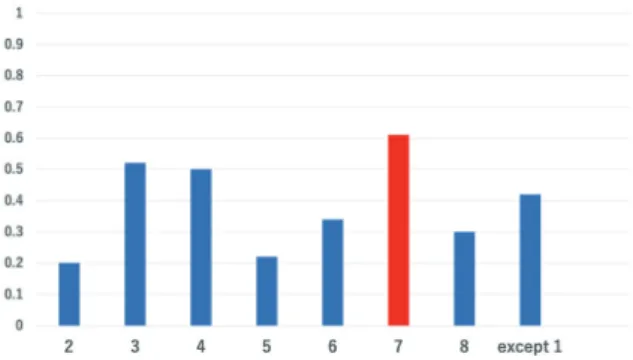
Similarly, for all other datasets, we confirmed that the proposed method selected the classifier with the highest recognition accuracy. Figure 5 shows the F-measure for each classifier when the dataset in home 1 is used as a test dataset. For the dataset in home 1, the proposed method selected the classifier shown by the red bar in Fig. 5. Classifier 7 had the highest recognition accuracy among the classifiers; hence, we can confirm that the classifier selection was performed correctly. Similarly, for all other datasets, we confirmed that the proposed method selected the classifier with the highest recognition accuracy.

5.2 Evaluation of classifier selection

To evaluate the effect of classifier selection, for each home, we performed the following three types of comparisons of the selected classifier with 1) the classifier trained on the entire dataset, 2) the classifier trained on a subset of the target home data, and 3) the rest of the classifiers, called infeasible classifiers, that were not selected because of low classifier fitness scores.

5.2.1 Classifier trained on entire training dataset

First, we compared our proposed method with a typical recognition model trained on the entire training dataset. Figure 6 shows the result of the comparison for each test dataset. For

each test dataset, the selected classifier can give a 1.5 to 1.7 times higher accuracy than the classifier using the entire training dataset.

5.2.2 Classifier trained on subset of target home data

Generally, if the model is trained on data from the same data source as the test dataset, the recognition accuracy increases because they have similar features. Therefore, it is important to compare the model trained on a subset of the dataset from the target home. Here, we investigated the recognition accuracy by fivefold cross-validation for each target home dataset for comparison with the proposed method.

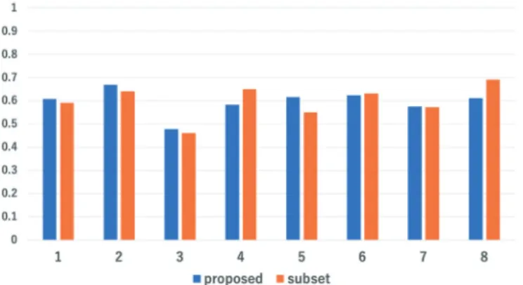
Figure 7 shows F-measures of the proposed method and the model trained on a subset of each target home dataset. According to the results, the proposed method gives an equivalent or higher recognition accuracy than does the model trained on a subset of the target home dataset. 5.3 Evaluation of learning algorithm

We also investigated how different models work in our algorithm. We used three types of machine learning algorithm: the balanced random forest (BRF),(27) SVM,(30) and AdaBoost.(31) In addition, we designed a rule-based approach based on our knowledge and compared it with other approaches. In this evaluation, we conducted leave-one-home-out cross-validation.

A rule-based approach is considered as a method of activity recognition from electricity consumption data. We have devised four simple rules to analyze the data and determine the activity by referring to the power fluctuations and time of day of each window.

(1) If the maximum value of power usage is not less than A watt, the activity is cooking.

(2) If the maximum value of power usage is not greater than B watts and the time is between X and Y o’clock, the activity is going-out.

(3) If the maximum value of power usage is not greater than B watts and the time is between Y and X o’clock, the activity is sleeping.

(4) Otherwise, the activity is others.

There are four thresholds, A, B, X, and Y, in the above rules. Regarding A, we empirically set 1000 as this value can commonly identify the cooking activities in most of the houses. The F-measure were evaluated by changing the values of B, X, and Y.

Table 5 shows the F-measure of the rule-based approach with variously changed thresholds. As a result, the accuracy was highest when B, X, and Y were 6, 18, and 100, respectively. When the threshold value was very large, sleeping and going out were often recognized as others, although sleeping and going out might also be recognized as others when the threshold value was very small because appliances with low power consumption, such as a refrigerator, were running all the time. The best result was only 0.25 since different households had different sleeping times and appliances that ran in the background while they slept, and it is not straightforward to determine reasonable rules that are applicable to many houses. We also compared the results with other learning methods with B, X, and Y as 6, 18, and 100, respectively.

Table 6 shows the precision, recall, and F-measure for each method obtained by cross-validation. Figure 8 shows the F-measure for each method for each home test dataset. Both Table 6 and Fig. 8 show that the method with the BRF has a higher accuracy than the rule-based, SVM, and AdaBoost methods for all datasets. Hence, we subsequently used the method with the BRF.

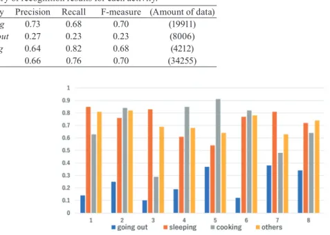
Table 7 shows the precision, recall, and F-measure for each activity obtained using the BRF. Figure 9 shows the F-measure for each activity for each test dataset. A recognition rate of approximately 70% was achieved for sleeping, cooking, and others by the proposed method. However, the proposed method gave a low recognition rate of 23% for going out. In most cases, going out was recognized as others. We consider that our proposed method could not recognize going out correctly because there was no clear difference in terms of power usage between going out and stay at home for elderly subjects.

5.4 Evaluation of time slot

We evaluated the accuracy of the data by changing the granularity of the data to take into account the case when the data were obtained at other intervals. In this experiment, we

Fig. 8. (Color online) F-measures for learning algorithms for each test. Table 5

Summary of recognition results for each threshold (A

= 1000). X,Y\B 10 100 300 5,17 0.24 0.24 0.17 6,18 0.24 0.25 0.18 7,19 0.24 0.25 0.17 Table 6

Summary of recognition results for each learning algorithm.

Method Precision Recall F-measure Rule-based 0.28 0.22 0.25

SVM 0.25 0.14 0.18

AdaBoost 0.49 0.51 0.48

BRF 0.61 0.60 0.59

Table 7

Summary of recognition results for each activity.

Activity Precision Recall F-measure (Amount of data)

sleeping 0.73 0.68 0.70 (19911)

going out 0.27 0.23 0.23 (8006)

cooking 0.64 0.82 0.68 (4212)

others 0.66 0.76 0.70 (34255)

Fig. 9. (Color online) Comparison of F-measures among activities for each test dataset.

changed the granularity of the data by removing samples to create 1- and 5-min-interval data. The F-measures of the BRF for households Nos. 1–8 using different interval data are shown in Fig. 10. The accuracy decreased with longer intervals, but the degree of decrease differed with household. Household No. 3 exhibited a marked decrease in F-measure, with many peaks in

20-s-interval data. This indicates that in 1-min-interval data, those peaks may disappear, and our method cannot identify the relevant activity, e.g., cooking. The number of households with an overall accuracy of less than 50% with 1-min-interval data was 3, and the average decrease in F-measure with 1-min-interval data was 10%. It is clearly shown that using 20-s-interval data achieved the highest F-measure.

6. Limitations and Discussion

Our proposed method was able to recognize activities except going out with an accuracy of about 70%. Although it is difficult to recognize exactly the activity in each time slot with this accuracy, it is possible to construct an approximate timetable for a day. As mentioned in Sect. 3.2, mental disease and kodokushi are related to the collapse of sleeping hours and eating habits. We consider that an accuracy of 100% is ideal, but it is not possible using only the low-resolution power usage data. For detecting disease precursors, our proposed method can distinguish unusual changes of life patterns.

We also aim to realize services such as a monitoring service using smart meters to estimate behaviors and monitor users’ activities. Therefore, the estimation of behaviors is performed using only aggregated low-frequency data sampled every 20 s. Therefore, it is not possible to observe the specific waveforms generated by home appliances at high frequencies, and it is not possible to estimate the type of home appliance in a precise manner. Furthermore, since the input is only electric power, reading and napping, which consume almost no electricity, cannot be distinguished. These problems can be solved by installing a device that can acquire high-frequency power waveforms or using sensors other than electricity power sensors. However, introducing the system into ordinary households is difficult because initial installation and maintenance costs will be incurred by the residents.

7. Conclusions

We proposed a low-cost, noninvasive method of recognizing activity patterns in the home using only the aggregate power consumption data measured periodically in the aggregated

power source by a smart meter. We provided a unique, data-driven approach, where the dataset obtained for 191 days from eight homes was used to build eight different classifiers, each of which was trained on one home dataset only. We also proposed a method of choosing the best-fit classifier based on the classifier best-fitness scores. Experimental results show that the proposed method achieved a recognition accuracy of 70% for several main ADLs.

As future work, we plan to collect more data from more homes to consider household diversity. We also plan to investigate the possible improvement of the algorithm. For example, we may apply a sliding window mechanism to estimate activities.

References

2 S.-W. Lee and K. Mase: IEEE Pervasive Comput. 1 (2002) 24.

3 L. Chen, C. D. Nugent, and H. Wang: IEEE Trans. Knowledge Data Eng. 24 (2012) 961.

4 X. Zhang, T. Kato, and T. Matsuyama: Proc. 2014 IEEE Innovative Smart Grid Technologies-Asia (IEEE, 2014) 73–78.

5 N. Rostamzadeh, G. Zen, I. Mironicã, J. Uijlings, and N. Sebe: Proc. Int. Conf. Image Analysis and Processing (Springer, 2013) 431–441.

6 K. Nakahara, H. Yamaguchi, and T. Higashino: Proc. 13th Int. Conf. Mobile and Ubiquitous Systems: Computing Networking and Services (2016) 106–111.

7 K. Ouchi and M. Doi: Proc. 2013 ACM Conf. Pervasive and Ubiquitous Computing Adjunct Publication (ACM, 2013) 103–106.

8 O. Brdiczka, M. Langet, J. Maisonnasse, and J. L. Crowley: IEEE Trans. Automation Sci. Eng. 6 (2009) 588. 9 H. Kalantarian, N. Alshurafa, T. Le, and M. Sarrafzadeh: Comput. Biol. Med. 58 (2015) 46.

10 T. Maekawa, Y. Kishino, Y. Sakurai, and T. Suyama: Proc. Int. Conf. Pervasive Computing (Springer, 2011) 276–293.

11 T. Van Kasteren, G. Englebienne, and B. J. Krӧse: Personal Ubiquitous Comput. 14 (2010) 489. 12 L. Chen, C. D. Nugent, and H. Wang: IEEE Trans. Knowl. Data Eng. 24 (2012) 961.

13 A. Fleury, M. Vacher, and N. Noury: IEEE Trans. Inf. Technol. Biomed. 14 (2010) 274.

14 S. Rollins and N. Banerjee: Proc. 2014 IEEE Int. Conf. Pervasive Computing and Communications (IEEE, 2014) 29–37.

15 K. Ueda, M. Tamai, Y. Arakawa, H. Suwa, and K. Yasumoto: Inf. Process. Soc. Jpn. Trans. 57 (2016) 416. 16 T. Mizumoto, K. Pattamasiriwat, Y. Arakawa, and K. Yasumoto: Proc. 2017 10th Int. Conf. Mobile Computing

and Ubiquitous Network (IEEE, 2017) 1–6.

17 S. N. Patel, T. Robertson, J. A. Kientz, M. S. Reynolds, and G. D. Abowd: Proc. Int. Conf. Ubiquitous Computing (Springer, 2007) 271–288.

18 C. Belley, S. Gaboury, B. Bouchard, and A. Bouzouane: Pervasive Mobile Comput. 12 (2014) 58. 19 S.-C. Lee, G.-Y. Lin, W.-R. Jih, and J. Y.-J. Hsu: Plan, Activity, and Intent Recognition (2010) pp. 37–44. 20 S. Biansoongnern and B. Plungklang: Proc. Comput. Sci. 86 (2016) 172.

21 C. Chalmers, P. Fergus, C. A. C. Montanez, S. Sikdar, F. Ball, and B. Kendall: IEEE Trans. Emerging Top. Comput. (2020).

22 Technology-bidgely: https://www.bidgely.com/technology/ (accessed 14 August 2020).

23 Ministry of Economy, Trade and Industry: A report from the smart meter system planning conference security review working group was compiled, https://www.meti.go.jp/english/press/2015/0710_01.html (accessed 14 August 2020).

24 B. Logan and J. Healey: Proc. 28th Annu. Int. Conf. Engineering in Medicine and Biology Society (IEEE, 2006) 5362–5365.

25 L. Anderson: Am. J. Geriatric Psychiatry 28 (2020) S128–S129.

26 A. S. Heller, T. C. Shi, CE C. Ezie, T. R. Reneau, L. M. Baez, C. J. Gibbons, and C. A. Hartley: Nat. Neurosci. (2020) 1–5.

27 A. L. C. Chen and L. Breiman: Tech. Rep. (2004) 666.

28 M. Wang, W. Li, and X. Wang: Proc. 2012 IEEE Conf. Computer Vision and Pattern Recognition (IEEE, 2012) 3274–3281.

29 Y. Honda, H. Yamaguchi, and T. Higashino: Proc. IEEE Annual Consumer Communications and Networking Conf. (IEEE, 2019) 1–6.

30 V. Vapnik and A. Lerner: Autom. Remote Control 24 (1963) 774. 31 Y. Freund and R. E. Schapire: J. Comput. Syst. Sci. 55 (1997) 119.

About the Authors

Kotaro Ishizu received his B.E. degree in information and computer sciences from Osaka University, Japan, in 2019. He is now an M.E. student under the supervision of Prof. Teruo Higashino in Mobile Computing Laboratory at Graduate School of Information Science and Technology, Osaka University.

Teruhiro Mizumoto received his B.E. degree from Kindai University, Japan, in 2009 and his M.E. and Ph.D. degrees from Nara Institute of Science and Technology, Japan, in 2011 and 2014, respectively. He was a postdoctoral fellow and assistant professor at Nara Institute of Science and Technology from 2016 to 2018. He became a specially appointed assistant professor (full time) at Graduate School of Information Science, Osaka University, Japan, in 2019. His current research interests are mental health monitoring, internet of things, and home automation. He is a member of IEEE and IPSJ.

Hirozumi Yamaguchi received his B.E., M.E., and Ph.D. degrees in information and computer sciences from Osaka University, Japan, in 1994, 1996, and 1998, respectively. He is currently an associate professor at Osaka University. His current research interests include the design, development, modeling, and simulation of mobile and wireless networks and applications. He is a member of the IEEE.

Teruo Higashino received his B.S., M.S., and Ph.D. degrees in information and computer sciences from Osaka University, Japan, in 1979, 1981, and 1984, respectively. He joined the faculty of Osaka University in 1984. Since 2002, he has been a professor in Graduate School of Information Science and Technology, Osaka University. His current research interests include the design and analysis of distributed systems, communication protocol, and mobile computing. He is a senior member of IEEE and a fellow of IPSJ.