LATENT GOLD CHOICE 4.0

(1)

USER’S GUIDE

Jeroen K. Vermunt

Jay Magidson

LATENT GOLD

®

CHOICE 4.0

Statistical

(2)

For more information about Statistical Innovations, Inc, please visit our website at http://www.statisticalinnovations.com or contact us at

Statistical Innovations, Inc. 375 Concord Avenue, Suite 007 Belmont, MA 02478

Latent GOLD® Choice is a trademark of Statistical Innovations Inc. Windows is a trademark of Microsoft Corporation.

SPSS is a trademark of SPSS, Inc.

Other product names mentioned herein are used for identification purposes only and may be trademarks of their respective companies.

No part of this publication may be reproduced or transmitted, in any form or by any means, electronic, mechanical, photocopying, recording, or otherwise, without the prior written permission from Statistical

Innovations Inc. 1/30/06 e-mail: will@statisticalinnovations.com

(3)

Manual for Latent GOLD Choice... 1

Structure of this manual ... 1

Part 1: Overview... 1

Latent GOLD Choice 4.0 Advanced ... 1

Optional Add-ons to Latent GOLD Choice 4.0... 2

Acknowledgments... 3

Part 2: Technical Guide for Latent GOLD Choice: Basic and Advanced……5

Introduction………..8

The Latent Class Model for Choice Data………..11

Estimation and Other Technical Issues……….30

The Latent GOLD Choice Output……….43

Introduction to Advanced Models……….59

Continuous Factors………60

Multilevel LC Choice Model……….…65

Complex Survey Sampling………72

Latent GOLD Choice's Advanced Output……….76

Bibliography………..80

Notation……….86

Part 3: Using Latent GOLD Choice ... 89

1.0 Overview ... 89

2.0 Introduction... 89

Step 1: Model Setup ...89

Model Analysis Dialog Box...92

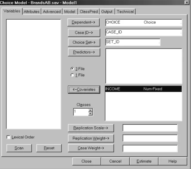
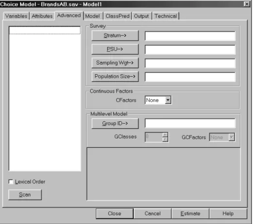
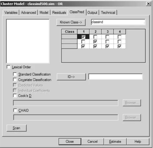
Variables Tab...93 Attributes Tab ...95 Advanced Tab...96 Model Tab... 100 ClassPred Tab ...101 Technical Tab ...103

Step 2: Specify Output Options ... 108

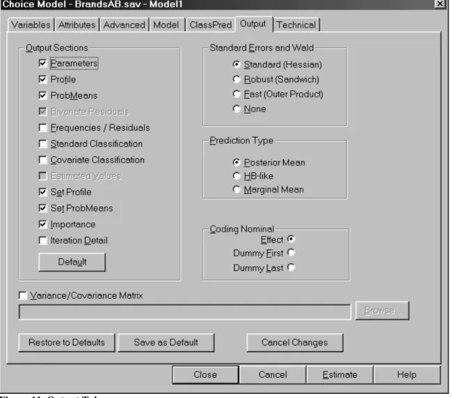
Output Tab ...108

ClassPred Tab ...112

Step 3: Estimate the Model ...114

Step 4: Viewing Output………..116

Output Options...116

Parameters Output...117

Importance...118

Profile View ...118

Profile Plot ...118

Profile Plot Settings ...118

ProbMeans View...119

Uni-Plot ...119

(4)

Set Profile and Set ProbMeans...120

Main Menu Options ...121

File Menu...121 Edit Menu ...121 View Menu ...121 Model Menu ...122 Window Menu...123 Help Menu ...123

(5)

Manual for Latent GOLD Choice 4.0

Structure of this manual

This manual consists of 3 Parts. Part 1 gives the overall general introduction to the program and new features.

Part 2, entitled the Technical Guide, documents all model options, technical features and output sections. It consists of 4 sections followed by a list of technical references. Section 1 presents a general introduction to the program. Section 2 contains several subsections which describe the various components of the model in formal mathematical terms, and provide examples of the various coding for the attributes. The last subsection (2.10) shows how all these components fit together in terms of the general latent class choice model. Section 3 describes the estimation, handling of missing data and other technical features. Section 4 provides the technical details for all of the output produced by the program.

Part 3 of the manual is entitled “Using Latent GOLD Choice”. It lists all menus and contains a detailed tutorial which takes you through the use of the program with actual applications. The tutorial also illustrates the use of the different data formats.

In addition to this manual, users may wish to refer to the Latent GOLD 4.0 User’s Guide, many of the details about the basic operation also apply to this program. That is, in addition to applying to the Cluster, DFactor and Regression modules of Latent GOLD 4.0 program, they also apply provide more complete operation details that also apply to Latent GOLD Choice 4.0

Part 1: Overview

Latent GOLD Choice is available as a stand-alone program or as an optional add-on module for Latent GOLD 4.0. An optional Advanced Module is also available as well as an optional link to the SI-CHAID profiling package. Latent GOLD Choice supports the following kinds of latent class choice models:

• First choice models – An extended multinomial logit model (MNL) is used to estimate the probability of making a specific choice among a set of alternatives as a function of choice attributes and individual characteristics (predictors).

• Ranking models – The sequential logit model is used for situations where a 1st and 2nd choice, 1st and last choice (best-worst), other partial rankings or choices from a complete ranking of all alternatives are obtained.

• Conjoint rating models – An ordinal logit model is used for situations where ratings of various alternatives, which may be viewed as a special kind of choice, are obtained.

For each of these situations, response data are obtained for one or more replications known as choice sets. Latent class (LC) choice models account for heterogeneity in the data by allowing for the fact that different population segments (latent classes) express different preferences in making their choices. For any application, separate models may be estimated that specify different numbers of classes. Various model fit statistics and other output are provided to compare these models to assist in determining the actual number of classes. Covariates may also be included in the model for improved description/ prediction of the segments.

Advanced program features include the use of various weights – case weights, replication weights, scale weights, and options to restrict the part-worth utility estimates in various ways. Some of the advanced applications include:

(6)

• Allocation models – Replication weights may be used to handle designs where respondents allocate a number of votes (purchases, points) among the various choice alternatives.

• Best-worst and related models -- A scale factor of ‘–1’ can be used to specify the alternative(s) judged to be worst (or least preferred) as opposed to best (or most preferred).

Latent GOLD Choice 4.0 Advanced

The following new features are included in the optional Advanced Module (requires the Advanced version) of Latent GOLD Choice 4.0:

• Continuous latent variables (CFactors) – an option for specifying models containing continuous latent variables, called CFactors, in a choice, ranking or rating model. CFactors can be used to specify random-coefficients conditional logit models, in which the random coefficients covariance matrix is restricted using a factor-analytic structure. It is also possible to use random-effects in conjunction with latent classes, yielding hybrid choice models combining discrete and continuous unobserved heterogeneity. If included, additional information pertaining to the CFactor effects appear in the Parameters, ProbMeans, and the Classification Statistics output and CFactor scores appear in the Standard Classification output.

• Multilevel modeling – an option for specifying LC choice models for nested data structures such as shoppers (individuals) within stores (groups). Group-level variation may be accounted for by specifying group-level latent classes (GClasses) and/or group-level CFactors (GCFactors). In addition, when 2 or more GClasses are specified, group-level covariates (GCovariates) can be included in the model to describe/predict them.

• Survey options for dealing with complex sampling data. Two important survey sampling designs are stratified sampling -- sampling cases within strata, and two-stage cluster sampling -- sampling within primary sampling units (PSUs) and subsequent sampling of cases within the selected PSUs. Moreover, sampling weights may exist. The Survey option takes the sampling design and the sampling weights into account when computing standard errors and related statistics associated with the parameter estimates, and estimates the ‘design. The parameter estimates are the same as when using the weight variable as a Case Weight when this method is used. An alternative two-step approach (‘unweighted’) proposed in Vermunt and Magidson (2001) is also available for situations where the weights may be somewhat unstable.

Additional Optional Add-ons to Latent GOLD Choice 4.0

The following optional add-on programs are also available that link to Latent GOLD Choice 4.0:

Latent GOLD 4.0

A license to Latent GOLD 4.0 allows you to use a single fully integrated latent class program that contains the Choice program as one module, and includes 3 additional modules to allow estimation of LC Cluster, DFactor (Discrete Factors) , and LC Regression models.

Numerous tutorials, and articles illustrate the use of these 3 kinds of models at

http://www.statisticalinnovations.com/products/latentgold_v4.html

In addition, the complete LG 4.0 User's Guide and a separate Technical Guide may also be downloaded.

(7)

With this option, a CHAID (CHi-squared Automatic Interaction Detector) analysis may be performed following the estimation of any LC Choice model, to profile the resulting LC segments based on demographics and/or other exogenous variables (Covariates). By selecting ‘CHAID’ as one of the output options, a CHAID input file is constructed upon completion of the model estimation, which can then be used as input to SI-CHAID 4.0.

This option provides an alternative treatment to the use of active and/or inactive covariates in Latent GOLD Choice 4.0. In addition to standard Latent GOLD output to examine the relationship between the covariates and classes/DFactors, SI-CHAID provides a tree-structured profile of selected classes/DFactors based on the selected Covariates. In addition, chi-square measures of statistical significance are provided for all covariates (Latent GOLD Choice does not provide such for inactive covariates).

Whenever covariates are available to describe latent classes obtained from Latent GOLD Choice 4.0, SI-CHAID 4.0 can be an especially valuable add-on tool under any of the following conditions:

• when many covariates are available and you wish to know which ones are most important

• when you do not wish to specify certain covariates as active because you do not wish them to affect the model parameters, but you still desire to assess their statistical significance with respect to the classes (or a specified subset of the classes)

• when you wish to develop a separate profile for each latent class (see Tutorial #1A)

• when you wish to explore differences between 2 or more selected latent classes using a tree modeling structure

• when the relationship between the covariates and classes is nonlinear or includes interaction effects, or

• when you wish to profile order-restricted latent classes

• For an example of the use of CHAID with Latent GOLD Choice 4.0, see Latent GOLD Choice Tutorial #1A on our website.

This option is especially useful in the development of simulators, as simulators can be easily extended to predict shares not only for each latent class segment, but also for CHAID segments defined using relevant exogeneous variables.

For further information on the CHAID add-on option, see:

http://www.statisticalinnovations.com/products/chaid_v4.html

DBMS/Copy interface

Latent GOLD Choice 4.0 reads SPSS, .cho and ASCII text files for data input. The DBMS/Copy interface allows Latent GOLD Choice 4.0 to directly open over 80 additional file formats, including Excel, SAS and HTML files. The full list of file formats is available at

http://www.statisticalinnovations.com/products/latentgold_80formats.html

Acknowledgments

We wish to thank the following people for supplying data: John Wurst (SDR Research), Wagner Kamakura (Duke University), Bryan Orme (Sawtooth Software).

We wish to that the following people for their helpful comments: Tom Eagle (Eagle Analytics), Steve Cohen (Cohen, Stratford), and Bengt Walerud (KW Partners).

We also wish to thank Michael Denisenko for assistance on this manual, and Alexander Ahlstrom for programming.

(8)

Technical Guide

for Latent GOLD Choice 4.0:

Basic and Advanced

1 Jeroen K. Vermunt and Jay Magidson

Statistical Innovations Inc.

(617) 489-4490

http://www.statisticalinnovations.com

1_{This document should be cited as “J.K. Vermunt and J. Magidson (2005).}

Techni-cal Guide for Latent GOLD Choice 4.0: Basic and Advanced. Belmont Massachusetts: Statistical Innovations Inc.”

(9)

Part I: Basic Model Options,

Technical Settings, and Output

Sections

1 Introduction to Part I (Basic Models)

Latent GOLD Choice is a program for the analysis of various types of pref-erence data; that is, data containing (partial) information on respondents’ preferences concerning one or more sets of alternatives, objects, options, or products. Such data can be obtained from different response formats, the most important of which are:

• first choice out of a set of M alternatives, possibly including a none option,

• paired comparison,

• full ranking of a set of M alternatives,

• partial ranking of a set of M alternatives,

• best and worst choices out of a set of M alternatives; also referred to as maximum-difference scaling,

• binary rating of a single alternative (positive-negative, yes-no, like-dislike),

• polytomous rating of a single alternative, e.g., on a 5-point scale,

• assigning a probability to a set of M alternatives; also referred to as constant-sum data,

• distribution of a fixed number of points (votes, chips, dollars, etc.) among a set ofM alternatives; also referred to as an allocation format,

• pick any out of a set of M alternatives,

• pick k (a prespecified number) out of a set of M alternatives, which is an example of what can be called a joint choice.

(13)

Latent GOLD Choice will accept each of these formats, including any com-bination of these.

The purpose of a discrete choice analysis is to predict stated or revealed preferences from characteristics of alternatives, choice situations, and respon-dents. The regression model that is used for this purpose is the conditional logit model developed by McFadden (1974). This is an extended multinomial logit model that allows the inclusion of characteristics of the alternatives – attributes such as price – as explanatory variables. Although the conditional logit model was originally developed for analyzing first choices, each of the other response formats can also be handled by adapting the basic model to the format concerned. For example, a ranking task is treated as a sequence of first choices, where the alternatives selected previously are eliminated; a rating task is modelled by an adjacent-category ordinal logit model, which is a special type of conditional logit model for ordinal outcome variables.

Latent GOLD Choice is not only a program for modeling choices or pref-erences, but also a program for latent class (LC) analysis. A latent class or finite mixture structure is used to capture preference heterogeneity in the population of interested. More precisely, each latent class corresponds to a population segment that differs with respect to the importance (or weight) given to the attributes of the alternatives when expressing that segment’s preferences. Such a discrete characterization of unobserved heterogeneity is sometimes referred to as a nonparametric random-coefficients approach (Aitkin, 1999; Laird, 1978; Vermunt, 1997; Vermunt and Van Dijk, 2001; Vermunt and Magidson, 2003). Latent GOLD Choice implements a non-parametric variant of the random-coefficient or mixed conditional logit model (Andrews et al., 2002; Louviere et al., 2000; McFadden and Train, 2000). The LC choice model can also be seen as a variant of the LC or mixture regression model (Vermunt and Magidson, 2000; Wedel and DeSarbo, 1994, 2002).

Most studies will contain multiple observations or multiple replications per respondent: e.g., respondents indicate their first choice for several sets of products or provide ratings for various products. This introduces depen-dence between observations. It is this dependepen-dence caused by the repeated measures that makes it possible to obtain stable estimates of the class-specific regression parameters.

A third aspect of the model implemented in Latent GOLD Choice is that class membership can be predicted from individual characteristics (covari-ates). In other words, one can not only identify latent classes, clusters, or segments that differ with respect to their preferences, but it is also

(14)

possi-ble to predict to which (unobserved) subgroup an individual belongs using covariates. Such a profiling of the latent classes substantially increases the practical usefulness of the results and improves out-of-study prediction of choices (Magidson, Eagle, and Vermunt, 2003; Natter and Feurstein, 2002; Vermunt and Magidson, 2002).

The next section describes the LC models implemented in Latent GOLD Choice. Then, attention is paid to estimation procedures and the correspond-ing technical options of the program. The output provided by the program is described in the last section.

Several tutorials are available to get you up and running quickly. These include:

• cbcRESP.sav - a simulated choice experiment

- Tutorial 1: Using LG Choice to Estimate Discrete Choice Models - Tutorial 2: Using LG Choice to Predict Future Choices

• brandABresp.sav - a simulated brand-price choice experiment - Tutorial 3: Estimating Brand and Price Effects

- Tutorial 4: Using the 1-file Format

• bank45.sav & bank9-1-file.sav - real data from a bank segmentation study

- Tutorial 5: Analyzing Ranking Data

- Tutorial 6: Using LG Choice to Estimate max-diff (best-worst) and Other Partial Ranking Models

• conjoint.sav, ratingRSP.sav, ratingALT.sav, ratingSET.sav: simulated data utilizing a 5-point ratings scale

- Tutorial 7: LC Segmentation with Ratings-based Conjoint Data - Tutorial 7A: LC Segmentation with Ratings-based Conjoint Data All of the above tutorials are available on our website at

(15)

2 The Latent Class Model for Choice Data

In order to be able to describe the models of interest, we first must clarify some concepts and introduce some notation. The data file contains infor-mation on I cases or subjects, where a particular case is denoted by i. For each case, there are Ti replications, and a particular replication is denoted by t. Note that in the Latent GOLD Choice interface, the Ti observations belonging to the same case are linked by means of a common Case ID.

Letyit denote the value of the dependent (or response) variable for case i at replication t, which can take on values 1 ≤ m ≤ M. In other words, M is number of alternatives and m a particular alternative. Three types of explanatory variables can be used in a LC choice model: attributes or characteristics of alternatives (zatt

itmp), predictors or characteristics of repli-cations (z_itqpre), and covariates or characteristics of individuals (zcov

ir ). Here, the indices p, q, andr are used to refer to a particular attribute, predictor, and covariate. The total number of attributes, predictors, and covariates is denoted by P, Q, and R, respectively. Below, we will sometimes use vector notation yi, zi, and zcov_i to refer to all responses, all explanatory variables, and all covariate values of case i, and zatt

it and z pre

it to refer to the attribute and predictor values corresponding to replication t for case i. Another vari-able that plays an important role in the models discussed below is the latent class variable denoted by x, which can take on values 1 ≤ x≤ K. In other words, the total number of latent classes is denoted by K.

Two other variables that may be used in the model specification are a replication-specific scale factorsit and a replication-specific weight vit. Their default values are one, in which case they do not affect the model structure.

2.1 First Choices

We start with the description of the regression model for the simplest and most general response format, first choice. For simplicity of exposition, we assume that each replication or choice set has the same number of alterna-tives. Later on it will be shown how to generalize the model to other formats, including choice sets with unequal numbers of alternatives.

A conditional logit model is a regression model for the probability that case i selects alternative m at replication t given attribute values zatt

it and predictor values zpre_it . This probability is denoted by P(yit = m|zattit ,z

pre it ). Attributes are characteristics of the alternatives; that is, alternative m will

(16)

have different attribute values than alternative m0. Predictors on the other hand, are characteristics of the replication or the person, and take on the same value across alternatives. For the moment, we assume that attributes and predictors are numeric variables. In the subsection “ Coding of Nominal Variables”, we explain in detail how nominal explanatory variables are dealt with by the program.

The conditional logit model for the response probabilities has the form P(yit=m|zattit ,z pre it ) = exp(ηm|zit) PM m0₌₁exp(η_m0_|_z it) ,

where ηm|zit is the systematic component in the utility of alternative m for

case iat replication t. The term ηm|zit is a linear function of an

alternative-specific constant β_mcon, attribute effects β_patt, and predictor effects β_mqpre (Mc-Fadden, 1974). That is,

ηm|zit =β con m + P X p=1

β_pattz_itmpatt + Q

X

q=1

β_mqprez_itqpre, where for identification purposes PM

m=1βmcon = 0, and

PM

m=1βmqpre = 0 for 1≤q≤Q, a restriction that is known as effect coding. It is also possible to use dummy coding using either the first or last category as reference category (see subsection 2.8). Note that the regression parameters corresponding to the predictor effects contain a subscript m, indicating that their values are alternative specific.

The inclusion of the alternative-specific constant βcon

m is optional, and models will often not include predictor effects. Without alternative-specific constants and without predictors, the linear model for ηm|zit simplifies to

ηm|zit =

P

X

p=1

β_pattz_itmpatt .

In a latent class or finite mixture variant of the conditional model, it is assumed that individuals belong to different latent classes that differ with respect to (some of) the β parameters appearing in the linear model for η (Kamakura and Russell, 1989). In order to indicate that the choice proba-bilities depend on class membership x, the logistic model is now of the form

P(yit =m|x,zattit ,z pre it ) = exp(ηm|x,zit) PM m0₌₁exp(η_m0_|_x,_z it) . (1)

(17)

Here, ηm|x,zit is the systematic component in the utility of alternative m at

replication tgiven that case i belongs to latent classx. The linear model for ηm|x,zit is ηm|x,zit =β con xm + P X p=1

β_xpattzatt_itmp+ Q

X

q=1

β_xmqpre z_itqpre. (2) As can be seen, the only difference with the aggregate model is that the logit regression coefficients are allowed to be Class specific.

In the LC choice model, the probability density associated with the re-sponses of case i has the form

P(yi|zi) = K X x=1 P(x) Ti Y t=1 P(yit|x,zattit ,z pred it ). (3)

Here, P(x) is the unconditional probability of belonging to Class xor, equiv-alently, the size of latent classx. Below, it will be shown that this probability can be allowed to depend an individual’s covariate values zcov

i , in which case P(x) is replaced by P(x|zcov_i ).

As can be seen from the probability structure described in equation (3), the Ti repeated choices of case i are assumed to be independent of each other given class membership. This is equivalent to the assumption of local independence that is common in latent variable models, including in the traditional latent class model (Bartholomew and Knott, 1999; Goodman, 1974a, 1974b; Magidson and Vermunt, 2004). Also in random-coefficients models, it is common to assume responses to be independent conditional on the value of the random coefficients.

2.2 Rankings and Other Situations with Impossible

Alternatives

In addition to models for (repeated) first choices, it is possible to specify models for rankings. One difference between first-choice and ranking data is that in the former there is a one-to-one correspondence between replications and choice sets while this is no longer the case with ranking data. In a ranking task, the number of replications generated by a choice sets equals the number of choices that is provided. A full ranking of a choice set consisting of five alternatives yields four replications; that is, the first, second, third, and fourth choice. Thus, a set consisting of M alternatives, generatesM−1

(18)

replications. This is also the manner in which the information appears in the response data file. With partial rankings, such as first and second choice, the number of replications per set will be smaller.

The LC model for ranking data implemented in Latent GOLD Choice treats the ranking task as sequential choice process (B¨ockenholt, 2002; Croon, 1989; Kamakura et al., 1994). More precisely, each subsequent choice is treated as if it were a first choice out of a set from which alternatives that were already selected are eliminated. For example, if a person’s first choice out of a set of 5 alternatives is alternative 2, the second choice is equivalent to a (first) choice from the 4 remaining alternatives 1, 3, 4, and 5. Say that the second choice is 4. The third choice will then be equivalent to a (first) choice from alternatives 1, 3, and 5.

The only adaptation that is needed for rankings is that it should be possible to have a different number of alternatives per set or, in our termi-nology, that certain alternatives are “impossible”. More precisely, M is still the (maximum) number of alternatives, but certain alternatives cannot be se-lected in some replications. In order to express this, we need to generalize our notation slightly. Let Ait denote the set of “possible” alternatives at replica-tion t for casei. Thus, ifm ∈Ait, P(yit =m|x,zattit ,z

pre

it ) is a function of the unknown regression coefficients, and if m /∈ Ait, P(yit =m|x,zattit ,z

pre it ) = 0. An easy way to accomplish this without changing the model structure is by setting ηm|x,zit = − ∞ for m /∈ Ait. Since exp(−∞) = 0, the choice

probability appearing in equation (1) becomes: P(yit =m|x,zattit ,z pre it ) = exp(ηm|x,zit) P m0_∈_A itexp(ηm0|x,zit) if m ∈ Ait and P(yit = m|x,zattit ,z pre

it ) = 0 if m /∈ Ait. As can be seen, the sum in the denominator is over the possible alternatives only.

When the dependent variable is specified to be a ranking variable, the specification of those alternatives previously selected as impossible alterna-tives is handled automatically by the program. The user can use a missing value in the sets file to specify alternatives as impossible. This makes it pos-sible to analyze choice sets with different numbers of alternatives per set, as well as combinations of different choice formats. In the one-file data format, choice sets need not have the same numbers of alternatives. In this case, the program treats “unused” alternatives as “impossible” alternatives.

(19)

2.3 Ratings

A third type of dependent variable that can be dealt with are preferences in the form of ratings. Contrary to a first choice or ranking task, a rating task concerns the evaluation of a single alternative instead of the comparison of a set of alternatives. Attributes will, therefore, have the same value across the categories of the response variable. Thus for rating data, it is no longer necessary to make a distinction between attributes and predictors.

Another important difference with first choices and rankings is that rat-ings outcome variables should be treated as ordinal instead of nominal. For this reason, we use an adjacent-category ordinal logit model as the regression model for ratings (Agresti, 2002; Goodman, 1979; Magidson, 1996). This is a restricted multinomial/conditional logit model in which the category scores for the dependent variable play an important role. Let y_m∗ be the score for category m. In most cases, this will be equally-spaced scores with mutual distances of one – e.g., 1, 2, 3, ... M, or 0, 1, 2, ... M−1 – but it is also pos-sible to use scores that are not equally spaced or non integers. Note that M is no longer the number of alternatives in a set but the number of categories of the response variable.

Using the same notation as above, the adjacent-category ordinal logit model can be formulated as follows

ηm|x,zit =β con xm +y ∗ m·   P X p=1

β_xpattz_itpatt+ Q

X

q=1

β_xqprez_itqpre

 .

The attribute and predictor effects are multiplied by the fixed category score y∗_m to obtain the systematic part of the “utility” of rating m . As can be seen, there is no longer a fundamental difference between attributes and predictors since attribute values and predictor effects no longer depend on m. For ratings, ηm|x,zit is defined by substituting y

∗

m · zitpatt in place of the category-specific attribute values z_itmpatt in equation (2), and the category-specific predictor effects βpre

xmq are replaced by y8m · βxqpre. The relationship between the category-specific utilities ηm|x,zit and the response probabilities

is the same as in the model for first choices (see equation 1).

As mentioned above, in most situations the category scoresy_m∗ are equally spaced with a mutual distance of one. In such cases, y_m∗ −y_m∗₋₁ = 1, and as result log P(yit=m|x,z att it ,z pre it ) P(yit =m−1|x,zattit ,z pre it ) = ηm|x,zit −ηm−1|x,zit

(20)

= β_xmcon−β_xcon₍_m₋₁₎ +

P

X

p=1

β_xpattz_itpatt+ Q

X

q=1

β_xqprez_itqpre.

This equation clearly shows the underlying idea behind the adjacent-category logit model. The logit in favor of rating m instead of m−1 has the form of a standard binary logit model, with an intercept equal to βcon

xm −βxcon(m−1) and slopes equal to βatt

xq and βxqpre. The constraint implied by the adjacent-category ordinal logit model is that the slopes are the same for each pair of adjacent categories. In other words, the attribute and predictor effects are the same for the choice between ratings 2 and 1 and the choice between ratings 5 and 4.

2.4 Replication Scale and Best-Worst Choices

A component of the LC choice model implemented in Latent GOLD Choice that has not been introduced thus far is the replication-specific scale factor sit. The scale factor allows the utilities to be scaled differently for certain replications. Specifically, the scale factor enters into the conditional logit model in the following manner:

P(yit=m|x,zattit ,z pre it , sit) = exp(sit ·ηm|x,zit) PM m0₌₁exp(s_it ·η_m0_|_x,_z it) .

Thus, it is seen that while the scale factor is assumed to be constant across alternatives within a replication, it can take on different values between repli-cations. The form of the linear model forηm|x,zit is not influenced by the scale

factors and remains as described in equation (2). Thus, the scale factor al-lows for a different scaling of the utilities across replications. The default setting for the scale factor issit= 1, in which case it cancels from the model for the choice probabilities.

Two applications of this type of scale factor are of particular importance in LC Choice modeling. The first is in the analysis of best-worst choices or maximum-difference scales (Cohen, 2003). Similar to a partial ranking task, the selection of the best and worst alternatives can be treated as a sequential choice process. The selection of the best option is equivalent to a first choice. The selection of the worst alternative is a (first) choice out of the remaining alternatives, where the choice probabilities are negatively related

(21)

to the utilities of these alternatives. By declaring the dependent variable to be a ranking, the program automatically eliminates the best alternative from the set available for the second choice. The fact that the second choice is not the second best but the worst can be indicated by means of a replication scale factor of -1, which will reverse the choice probabilities. More precisely, for the worst choice,

P(yit=m|x,zattit ,z pre it , sit) = exp(−1·ηm|x,zit) P m0_∈_A itexp(−1·ηm0|x,zit) if m ∈Ait and 0 if m /∈Ait.

The second noteworthy application of the scale factor occurs in the si-multaneous analysis of stated and revealed preferences. Note that use of a scale factor larger than 0 but smaller than 1 causes sit·ηm|x,zit to be shrunk

compared to ηm|x,zit and as a result, the choice probabilities become more

similar across alternatives. A well-documented phenomenon is that stated preferences collected via questionnaires yield more extreme choice probabil-ities than revealed preferences (actual choices) even if these utilprobabil-ities are the same (Louviere et al., 2000). A method to transform the utilities for these two data types to the same scale is to use a somewhat smaller scale factor for the revealed preferences than for the stated preferences. Assuming that the scale factor for the stated preferences is 1.0, values between 0.5 and 1.0 could be tried out for the revealed preferences; for example,

P(yit =m|x,zattit ,z pre it , sit) = exp(0.75·ηm|x,zit) PM m0₌₁exp(0.75·η_m0_|_x,_z it) .

A limitation of the scale factor implemented in Latent GOLD Choice is that it cannot vary across alternatives. However, a scale factor is nothing more than a number by which the attributes (and predictors) are multiplied, which is something that users can also do themselves when preparing the data files for the analysis. More precisely, the numeric attributes of the alternatives may be multiplied by the desired scale factor.

2.5 Replication Weight and Constant-sum Data

The replication weights vit modify the probability structure defined in equa-tion (3) as follows: P(yi|zi) = K X x=1 P(x) Ti Y t=1 h P(yit|x,zattit ,z pred it ) ivit .

(22)

The interpretation of a weight is that choice yit is made vit times.

One of the applications of the replication weight is in the analysis of constant-sum or allocation data. Instead of choosing a single alternative out of set, the choice task may be to attach a probability to each of the alternatives. These probabilities serve as replication weights. Note that with such a response format, the number of replications corresponding to a choice set will be equal to the number of alternatives. A similar task is the distribution of say 100 chips or coins among the alternatives, or a task with the instruction to indicate how many out of 10 visits of a store one would purchase each of several products presented.

Other applications of the replication weights include grouping and differ-ential weighting of choices. Grouping may be relevant if the same choice sets are offered several times to each observational unit. Differential weighting may be desirable when analyzing ranking data. In this case, the first choice may be given a larger weight in the estimation of the utilities than subse-quent choices. It is even possible to ask respondents to provide weights – say between 0 and 1 – to indicate how certain they are about their choices. In the simultaneous analysis of stated and revealed preference data, it is quite common that several stated preferences are combined with a single revealed preference. In such a case, one may consider assigning a higher weight to the single revealed preference replication to make sure that both preference types have similar effects on the parameter estimates.

2.6 Other Choice/Preference Formats

In the previous sections, we showed how to deal with most of the response for-mats mentioned in the introduction. To summarize, first choice is the basic format, rankings are dealt with as sequences of first choices with impossi-ble alternatives, ratings are modelled by an ordinal logit model, best-worst choices can be treated as partial rankings with negative scale factors for the second (worst) choice, and the analysis of constant-sum data involves the use of replications weights.

A format that has not been discussed explicitly is paired comparisons (Dillon and Kumar, 1994). Paired comparisons are, however, just first choices out of sets consisting of two alternatives, and can therefore be analyzed in the same way as first choices. Another format mentioned in the introduction is binary rating. Such a binary outcome variable concerning the evaluation of a single alternative (yes/no, like/dislike) can simply be treat as a rating. The

(23)

most natural scoring of the categories would be to use score 1 for the positive response and 0 for the negative response, which yields a standard binary logit model. The pick any out of M format can be treated in the same manner as binary ratings; that is, as a set of binary variables indicating whether the various alternatives are picked or not.

Another format, called joint choices, occurs if a combination of two or more outcome variables are modelled jointly. Suppose the task is to give the two best alternatives out of a set of M, which is a pick 2 out of M format. This can be seen as a single choice with M ·(M −1)/2 joint alternatives. The attribute values of these joint alternatives are obtained by summing the attribute values of the original pair of alternatives. Other examples of joint choices are non-sequential models for rankings (B¨ockenholt, 2002; Croon, 1989) and best-worst choices (Cohen, 2003). For example, a pair of best and worst choices can also be seen as a joint choice out of M ·(M − 1) joint alternatives. The attribute values of these joint alternatives are equal to the attribute values of the best minus the attributes of the worst. What is clear from these examples is that setting up a model for a joint choice can be quite complicated.

Another example of a situation in which one has to set up a model for a joint response variable is in capture-recapture studies (Agresti, 2002). For the subjects that are captured at least ones, one has information on capture at the various occasions. The total number of categories of the joint dependent variable is 2T ₋_{1, where} _T _{is the number of time point or replications.}

Note that these examples of joint choice models all share the fact that the number of possible joint alternatives is smaller than the product of the number of alternatives of the separate choices. That is, in each case, certain combinations of choices are impossible, and hence the model of interest can-not be set up as a series of independent choices. Instead, these situations should be specified as a single joint choice.

The last “choice format” we would like to mention is the combination of different response formats. The most general model is the model for first choices. Models for rankings and ratings are special cases that are obtained by adapting the model for first choices to the response format concerned. This is done internally (automatically) by the program. It is, however, also possible to specify ranking or rating models as if they were models for first choices. In the ranking case, this involves specifying additional choice sets in which earlier selected alternatives are defined as “impossible”. A rating model can be specified as a first choice model by defining the categories of

(24)

the dependent variable as alternatives with attribute values zatt

itpm equal to y∗_m· z_itpatt.

Given the fact that each of the response formats can be treated as a first choice, it is possible to make any combination of the formats that were discussed. Of course, setting up the right alternatives and sets files may be quite complicated. An issue that should be taken into account when using combinations of response formats is the scaling of the replications. For example, it might be that the utilities should be scaled in a different manner for ratings than for first choices.

2.7 Covariates

In addition to the explanatory variables that we called attributes and pre-dictors, it is also possible to include another type of explanatory variable – called covariates – in the LC model. While attributes and predictors enter in the regression model for the choices, covariates are used to predict class membership. In the context of LC analysis, covariates are sometimes referred to as concomitant or external variables (Clogg, 1981; Dayton and McReady, 1988; Kamakura et al., 1994; Van der Heijden et al., 1996).

When covariates are included in the model, the probability structure changes slightly compared to equation (3). It becomes

P(yi|zi) = K X x=1 P(x|zcov_i ) Ti Y t=1 P(yit|x,zattit ,z pred it ). (4)

As can be seen, class membership of individual i is now assumed to depend on a set of covariates denoted by zcov

i . A multinomial logit is specified in which class membership is regressed on covariates; that is,

P(x|zcov_i ) = exp(ηx|zi)

PK

x0₌₁exp(η_x0_|_z

i)

, with linear term

ηx|zi =γ0x+

R

X

r=1

γrxzcovir . (5)

Here, γ0x denotes the intercept or constant corresponding to latent class x and γrx is the effect of the rth covariate for Class x. Similarly to the model for the choices, for identification, we either set PK

(25)

γrK = 0 for 0 ≤ r ≤ R, which amounts to using either effect or dummy coding. Although in equation (5) the covariates are assumed to be numeric, the program can also deal with nominal covariates (see subsection 2.8).

We call this procedure for including covariates in a model the “active covariates method”: Covariates are active in the sense that the LC choice solution with covariates can be somewhat different from the solution with-out covariates. An alternative method, called “inactive covariates method”, involves computing descriptive measures for the association between covari-ates and the latent variable after estimating a model without covariate effects. More detail on the latter method is given in the subsection explaining the Profile and ProbMeans output.

Another approach that can be used to explore the relationship between covariates and the latent variable is through the use of the CHAID option. This option may be especially valuable when the goal is to profile the latent classes using many inactive covariates. This option requires the SI-CHAID 4.0 add-on program, which assesses the statistical significance between each covariate and the latent variable. For further information about the CHAID option see Section 4.9.

2.8 Coding of Nominal Variables

In the description of the LC choice models of interest, we assumed that attributes, predictors, and covariates were all numeric. This limitation is not necessary however, as Latent GOLD Choice allows one or more of these explanatory variables to be specified to be nominal. For nominal variables, Latent GOLD Choice sets up the design vectors using either effect (ANOVA-type) coding or dummy coding with the first or last category as reference category for identification. Effect coding means that the parameters will sum to zero over the categories of the nominal variable concerned, In dummy coding, the parameters corresponding to the reference category are fixed to zero.

Suppose we have a nominal attribute with 4 categories in a model for first choices. The effect coding constraint implies that the corresponding 4 effects should sum to 0. This is accomplished by defining a design matrix with 3 numeric attributes zatt

(26)

for the 3 non-redundant terms (βatt

x1, βxatt2, βxatt3) is as follows: category 1 category 2 category 3 category 4 1 0 0 0 1 0 0 0 1 −1 −1 −1 ,

where each row corresponds to a category of the attribute concerned and each column to one of the three parameters. Although the parameter for the last category is omitted from model, you do not notice that because it is computed by the program after the model is estimated. The parameter for the fourth category equals −P3

p=1βxpatt; that is, minus the sum of the parameters of the three other categories. This guarantees that the parameters sum to zero since

P3

p=1βxpatt−

P3

p=1βxpatt = 0.

Instead of using effect coding, it is also possible to use dummy coding. Depending on whether one uses the first or the last category as reference category, the design matrix will look like this

category 1 category 2 category 3 category 4 0 0 0 1 0 0 0 1 0 0 0 1 . or this category 1 category 2 category 3 category 4 1 0 0 0 1 0 0 0 1 0 0 0 .

Whereas in effect coding the category-specific effects should be interpreted in terms of deviation from the average, in dummy coding their interpretation is in terms of difference from the reference category. Note that the parameter for the reference category is omitted, which implies that it is equated to 0.

It also possible to work with user specified coding schemes. An example is category 1 category 2 category 3 category 4 0 0 0 1 0 0 1 1 0 1 1 1 ,

(27)

which yields parameters that can be interpreted as differences between ad-jacent categories. More precisely, β_xatt₁ is the difference between categories 2 and 1, β_xatt₂ between categories 3 and 2, and β_xatt₃ between categories 4 and 3. As explained in the previous sections, the effect and dummy coding straints are not only imposed on the attribute effects, but also on the con-stants and the predictor effects in the regression model for first choices and rankings, on the constants in the regression model for ratings, and on the intercepts and covariate effects in the regression model for the latent classes.

2.9 Known-Class Indicator

Sometimes, one has a priori information – for instance, from an external source – on the class membership of some individuals. For example, in a four-class situation, one may know that case 5 belongs to latent four-class 2 and case 11 to latent class 3. Similarly, one may have a priori information on which class cases do not belong to. For example, again in a four-class situation, one may know that case 19 does not belong to latent class 2 and that case 41 does not belong to latent classes 3 or 4. In Latent GOLD, there is an option – called “Known Class” – for indicating to which latent classes cases donot belong to.

Let τi be a vector of 0-1 variables containing the “Known Class” infor-mation for case i, where τix = 0 if it is known that case i does not belong to class x, and τix = 1 otherwise. The vector τi modifies the model with covariates defined in equation (4) as follows:

P(yi|zi,τi) = K X x=1 τixP(x|zcovi ) Ti Y t=1 P(yit|x,zattit ,z pred it ).

As a result of this modification, the posterior probability of belonging to class x will be equal to 0 if τix = 0.

The known-class option has three important applications.

1. It can be used to estimate models with training cases; that is, cases for which class membership has been determined using a gold standard method. Depending on how this training information is obtained, the missing data mechanism will be MCAR (Missing Completely At Ran-dom, where the known-class group is a random sample from all cases), MAR (Missing At Random, where the known-class group is a random sample given observed responses and covariate values), or NMAR (Not

(28)

Missing At Random, where the known-class group is a non-random sample and thus may depend on class membership itself). MAR oc-curs, for example, in clinical applications in which cases with more than a certain number of symptoms are subjected to further examination to obtain a perfect classification (diagnosis). NMAR may, for example, occur if training cases that do not belong to the original sample under investigation are added to the data file.

Both in the MAR and MCAR situation, parameter estimates will be un-biased. In the NMAR situation, however, unbiased estimation requires that separate class sizes are estimated for training and non-training cases (McLachlan and Peel, 2000). This can easily be accomplished by expanding the model of interest with a dichotomous covariate that takes on the value 0 for training cases and 1 for non-training cases. 2. Another application is specifying models with a partially missing

dis-crete variable that affects one or more response variables. An important example is the complier average causal effect (CACE) model proposed by Imbens and Rubin (1997), which can be used to determine the effect of a treatment conditional on compliance with the treatment. Compli-ance is, however, only observed in the treatment group, and is missing in the control group. This CACE model can be specified as a model in which class membership (compliance) is known for the treatment group, and which a treatment effect is specified only for the compliance class. 3. The known-class indicator can also be used to specifymultiple-group LC models. Suppose we have a three-class model and two groups, say males and females. A multiple-group LC model is obtained by indicating that there are six latent classes, were males may belong to classes 1–3 and females to classes 4–6. To get the correct output, the grouping variable should not only be used as the known-class indicator, but also as a nominal covariate.

2.10 Zero-Inflated Models

When the zero-inflated option is used, the model is expanded withM latent classes that are assumed to respond with probability one to a certain cate-gory; that is, P(yit =m|x,z

pred

(29)

sometimes referred to as stayer classes (in mover-stayer models) or brand-loyal classes (in brand-brand-loyalty models).

2.11 Restrictions on the Regression Coefficients

Various types of restrictions can be imposed on the Class-specific regression coefficients: attribute and predictor effects can be fixed to zero, restricted to be equal across certain or all Classes, and constrained to be ordered. More-over, the effects of numeric attributes can be fixed to one. These constraints can either be used as a priori restrictions derived from theory or as post hoc restrictions on estimated models.

Certain restrictions apply to parameters within each Class, while others apply across Classes. The within-Class restrictions are:

• No Effect: the specified effect(s) are set to zero;

• Offset: the selected effect(s) are set to one, thus serving as an offset.2 The offset effect applies to numeric attributes only.

Between-Class restrictions are:

• Merge Effects: the effects of a selected attribute/predictor are equated across 2 or more specified Classes;

• Class Independent: the effects of a selected attribute/predictor are equated across all Classes;

• Order (ascending or descending): in each Class, the effect of a selected numeric attribute/predictor is assumed to have the same sign or the effects corresponding to a selected nominal attribute/predictor are as-sumed to be ordered (either ascending or descending). That is, for numeric attributes/predictors, the ascending restriction implies that the Class-specific coefficients should be at least zero (β ≥ 0) and the descending restriction that they are at most zero (β ≤0). For nominal attributes/predictors, ascending implies that the coefficient of category

2_{The term offset stems from the generalized linear modeling framework. It refers to}

a regression coefficient that is fixed to 1, or equivalently, to a component that offsets the linear part of the regression model by a fixed amount. An offset provides the same role as a cell weight in log-linear analysis. An offset is in fact, the log of a cell weight.

(30)

p+ 1 is larger than or equal to the one of category p (βp ≤ βp+1, for eachp) and descending that the coefficient of category p+ 1 is smaller than or equal to the one of category p(βp ≥βp+1, for each p).

The “Class Independent” option can be used to specify models in which some attribute and predictor effects differ across Classes while others do not. This can either be on a priori grounds or can be based on the test statistics from previously estimated models. More specifically, if the Wald(=) test is not significant, it makes sense to check whether an effect can be assumed to be Class independent.

There is a special variant of the Class-independent option called “No Sim-ple” that can be used in conjunction with the constants in a rating model. With this option, the constants are modeled asβcon

xm =β·conm +βxcon· ·ym∗, where β_xcon_· is subjected to an effect or dummy coding constraint. This specification of Class-specific constants is much more parsimonious and is, in fact, equiv-alent to how x-y relationships with ordinal y’s are modeled in LC Cluster models. Rather that estimating K ·M intercept terms, one now estimates only M +K −1 coefficients; that is, one extra coefficient per extra latent class.

“Order” constraints are important if one has a priori knowledge about the sign of an effect. For example, the effect of price on persons’ preferences is usually assumed to be negative – or better, non-positive – for each latent class (segment). If the price effect is specified to be “Descending”, the result-ing parameter estimate(s) will be constrained to be in agreement with this assumption.

The “No Effect” option makes it possible to specify a different regression equation for each latent class. More specifically, each latent class may have different sets of attributes and predictors affecting the choices. Post hoc constraints can be based on the reported z value for each of the coefficients. An example of an a priori use of this constraint is the inclusion of a random-responder class, a class in which all coefficient are zero. This is specified as follows:

Constants Attribute1 Attribute2

Class 1 Class 2 Class 3 Class 4

− 2 3 4

,

where “−” indicates that the effect is equal to 0. In this example, Class 1 is the random-responder class.

(31)

“Merge Effects” is a much more flexible variant of “Class Independent”. It can be used to equate the parameters for any set of latent classes. Besides post hoc constraints, very sophisticated a priori constraints can be imposed with this option. An important application is the specification of LC DFactor structures in which each latent class corresponds to the categories of two or more latent variables. For example, consider a set of constraints of the form:

Constants Attribute1 Attribute2

1 1 3 3

1 2 1 2

,

where the same numbers in a given row indicate that the associated class pa-rameters are equal. This restricted 4-Class model is a 2-dimensional DFactor model: the categories of DFactor 1 differ with respect to the constants and the categories of DFactor 2 with respect to the two attribute effects. Specifi-cally, level 1 of DFactor 1 is formed by Classes 1 and 2 and level 2 by Classes 3 and 4; level 1 of DFactor 2 is formed by Classes 1 and 3 and level 2 by Classes 2 and 4.

The option “Offset” can be used to specify any nonzero fixed-value con-straint on the Class-specific effect of a numeric attribute. This means that it is possible to refine the definition of any Class (segment) by enhancing or reducing the estimated part-worth utility of any numeric attribute for that Class. Recall that numeric attribute p enters as βatt

xp zitmpatt in the linear part of the conditional logit model. Suppose, after estimating the model, the es-timate for βatt

xp turned out to be 1.5 for Class 1. If zattitmp is specified to be an offset, the importance of this attribute to be reduced (1.5 would be reduced to 1) for this Class. But suppose that you wish to enhance the importance of this attribute for Class 1; say, you wish to restrict βatt

xp to be equal to 2. The trick is to recode the attribute, replacing each code by twice the value. Thus, the recoded attribute is defined as 2·z_itmpatt . If we restrict the effect of this recoded attribute to 1, we obtain 1·2·zatt

itmp, which shows that the effect of zatt

itmp is equated to 2. Such recoding can be done easily within Latent GOLD Choice, using the Replace option.

In addition to post hoc refinements to customize the definition of the resulting latent classes, the offset restriction can also be used to make the Classes conform to various theoretical structures. Probably the most impor-tant a priori application of “Offset” is that of defining stayer- or brand-loyal classes. A brand-loyal class selects one of the brands with a probability equal

(32)

to 1 and is not affected by the other attributes. An example of a restrictions table corresponding to such a structure is:

Brand1(100) Brand2(100) Brand3(100) Constants Attribute1 Attribute2

∗ − − − − ∗ − − − − ∗ − − − − 4 − − − 4 − − − 4 .

Here, “−” means no effect and “∗” means offset. As can be seen, Classes 1, 2, and 3 are only affected by an offset, and Class 4 – the brand-switching or mover class – is affected by the constants and the two attributes. The numeric “attributes” Brand1(100), Brand2(100), and Brand3(100) are brand “dummies” that take on the value 100 for the brand concerned and are 0 otherwise.3 As a result of the fixed effect of 100, the probability of selecting the corresponding brand will be equal to one. To illustrate this, suppose that a choice set consists of three alternatives and that (only) alternative 1 is associated with brand 1. The probability that someone belonging to Class 1 selects alternative 1 equals exp(100)/[exp(100) + exp(0) + exp(0)] = 1.0000.4 _{Although this model is similar to a zero-inflated model, the} offset-based specification is much more flexible in the sense that the number of brand-loyal classes does not need to coincide with the number of alternatives per set. In the above example, the sets could consist of four instead of three alternatives, say three different brands and a “none” alternative.

Now, we will discusses several more advanced applications of the restric-tion oprestric-tions. The first is a model for ratings with a parsimonious specificarestric-tion of the Class dependence of the constants. Let “One” be an attribute with the constant value l. The model of interest is obtained with the restrictions

3_{It is not necessary to assume that the 100 appears in all alternatives for the brand}

concerned. The value could also be 100 if a particular condition is fulfilled – for example, if the price of the evaluated product is larger than a certain amount – and 0 otherwise. This shows that the offset option provides a much more flexible way of specifying classes with zero response probabilities than the zero-inflated option.

4_{While a value of 100 for the offset can be used to fix a probability to 1.0000, a value}

of -100 can be use to fix a probability to 0.0000. For example, exp(−100)/[exp(−100) + exp(0) + exp(0)] = 0.0000.

(33)

table

Constants One Attribute1 Attribute2

1 1 1 1

− 2 3 4

1 2 3 4

.

Instead of having a separate set of constants for each latent class, the re-stricted constant for category m in Class x equals βcon

xm = βmcon +y

∗

m ·βxatt1, where for identification, βatt

11 = 0. Note that this is equivalent to using the ”no-simple” setting for the constants and similar to the treatment of ordinal indicators in the LC Cluster and DFactor Modules of Latent GOLD.

Suppose you assume that the effect of price is negative (descending) for Classes 1-3 and unrestricted for Class 4. This can be accomplished by having two copies of the price variable in the model, say Price1 and Price2. The effect of Price1 is specified as ordered and is fixed to zero in Class 4. The effect of Price2 is fixed to zero in Classes 1-3.

Suppose your assumption is that the effect of a particular attribute is at least 2. This can be accomplished by combining a fixed value constraint with an order constraint. More precisely, an additional attribute defined as 2·zatt

itmpis specified to be an offset and the effect of the original attributezitmpatt defined to be ascending.

Our final example is an exploratory variant of the DFactor structure de-scribed above. Suppose you want a two-DFactor model without assumptions on which discrete factor influences which attribute effects. This can be ac-complished having 3 copies of all attributes in the attributes file. With two attributes (brand and price), the restriction table is of the form

Brand1 Brand2 Brand3 Price1 Price2 Price3

1 1 1 1 − − 3 3 − 2 − 2 1 1 1 1 − − 3 3 − 2 − 2 .

The first copy (Brand1 and Price1) defines a main effect for each attribute. The second copy (Brand2 and Price2) is used to define the first DFactor, a contrast between Classes 3/4 and 1/2. The third copy (Brand3 and Price3) specifies DFactor 2 by means of a contrast between Classes 2/4 and 1/3.

(34)

2.12 General Latent Class Choice Model

In the previous subsections, we described the various elements of the LC model implemented in Latent GOLD Choice. Now, we will combine all these elements and provide the structure of the general LC choice model. The general probability density function associated with case iis

it ) are parameterized by logit mod-els; that is,

ηx|zi =γ0x+

R

X

r=1

γrxzcovir . For first choices and rankings, ηm|x,zit equals

ηm|x,zit =β con xm + P X p=1

β_xpattzatt_itmp+ Q

X

q=1

β_xmqpre z_itqpre, if m ∈Ait and −∞ otherwise. For ratings,

ηm|x,zit =β con xm +y ∗ m·   P X p=1

β_xpattz_itpatt+ Q

X

q=1

β_xqprez_itqpre

 .

3 Estimation and Other Technical Issues

3.1 Log-likelihood and Log-posterior Function

The parameters of the LC choice model are estimated by means of Maximum Likelihood (ML) or Posterior Mode (PM) methods. The likelihood function

(35)

is derived from the probability density function defined in equation (6). Let

ϑ denote the vector containing theγ and β parameters. As before, yi andzi denote the vectors of dependent and explanatory variables for case i, and I denotes the total number of cases.

ML estimation involves finding the estimates for ϑ that maximize the log-likelihood function logL= I X i=1 wilogP(yi|zi, ϑ).

Here, P(yi|zi, ϑ) is the probability density associated with case i given pa-rameter values ϑ and wi is the Case Weight corresponding to case i.5 This case weight wi can be used to group identical response patterns or to specify (complex survey) sampling weights. In the former case, wi will serve as a frequency count, and in the latter case, Latent GOLD Choice will provide pseudo ML estimates (Patterson, Dayton, and Graubard, 2002).6 _{The other} type of weight –Replication Weight vit – that was introduced in the previous section modifies the definition of the relevant probability densityP(yi|zi, ϑ). The exact form of P(yi|zi, ϑ) is described in equation (6).

In order to prevent boundary solutions or, equivalently, to circumvent the problem of non-existence of ML estimates, we implemented some ideas from Bayesian statistics in Latent GOLD Choice. The boundary problem that may occur is that the (multinomial) probabilities of the model for the latent classes or the model for the choices, rankings, or ratings may converge to zero. This occurs if a β or γ parameter becomes very extreme, tends to go to (minus) infinity. The boundary problem is circumvented by using Dirichlet priors for the latent and the response probabilities (Clogg et al., 1991; Galindo-Garre, Vermunt, and Bergsma, 2004; Gelman et. al., 1996; Schafer, 1997). These are so-called conjugate priors since they have same form as the corresponding multinomial probability densities. The implication of using priors is that the estimation method is no longer ML but PM (Posterior Mode).

Denoting the assumed priors for ϑ by p( ϑ) and the posterior by P, PM estimation involves finding the estimates for ϑ that maximize the

log-5_{In order to simplify the discussion, in this section we discuss only on the situation}

without known-class indicators.

6_{In Latent GOLD Choice Advanced, there is a more elegant option for dealing with}

(36)

posterior function

logP = logL+ logp(ϑ) =

I

X

i=1

wilogP(yi|zi, ϑ) + logp(ϑ), or, in other words, finding the point where ∂logP

∂ϑ = 0. Algorithms that are used to solve this problem – EM and Newton-Raphson – are described below. The user-defined parameters in the priors p(ϑ) can be chosen in such a way that logp(ϑ) = 0, which makes PM estimation turn into ML estimation. PM estimation can also be seen as a form of penalized ML estimation, in which p(ϑ) serves as a function penalizing solutions that are too near to the boundary of the parameter space and, therefore, smoothing the estimates away from the boundary.

3.2 Missing Data

3.2.1 Dependent variable

If the value of the dependent variable is missing for one or more of the replica-tions of casei, the replications concerned are omitted from the analysis. The remaining replications will, however, be used in the analysis. Thus, instead of using list-wise deletion of cases, Latent GOLD Choice provides ML or PM estimates based on all available information. The assumption that is made is that the missing data are missing at random (MAR) or, equivalently, that the missing data mechanism is ignorable (Little and Rubin, 1987; Schafer, 1997; Skrondal and Rabe-Hesketh, 2004; Vermunt, 1997).

In the case of missing data, it is important to clarify the interpretation of the chi-squared goodness-of-fit statistics. Although parameter estimation with missing data is based on the MAR assumption, the chi-squared statistics not only test whether the model of interest holds, but also the much more restrictive MCAR (missing completely at random) assumption (see Vermunt, 1997). Thus, caution should be used when interpreting the overall goodness-of-fit tests in situations involving missing data.

3.2.2 Attributes, predictors, and covariates

Missing values on attributes will never lead to exclusion of cases or replica-tions from the analysis. If the technical option for including missing values

LATENT GOLD CHOICE 4.0

USER’S GUIDE

USER’S GUIDE

Jeroen K. Vermunt

Jay Magidson

LATENT GOLD

®

CHOICE 4.0

Statistical

TABLE OF CONTENTS

Manual for Latent GOLD Choice... 1

Part 1: Overview... 1

Part 2: Technical Guide for Latent GOLD Choice: Basic and Advanced……5

Part 3: Using Latent GOLD Choice ... 89

Manual for Latent GOLD Choice 4.0

Technical Guide

for Latent GOLD Choice 4.0:

Basic and Advanced

1

Jeroen K. Vermunt and Jay Magidson

Contents

Part I: Basic Model Options,

Technical Settings, and Output

Sections

1

Introduction to Part I (Basic Models)

2

The Latent Class Model for Choice Data

2.1

First Choices

2.2

Rankings and Other Situations with Impossible

Alternatives

2.3

Ratings

2.4

Replication Scale and Best-Worst Choices

2.5

Replication Weight and Constant-sum Data

2.6

Other Choice/Preference Formats

2.7

Covariates

2.8

Coding of Nominal Variables

2.9

Known-Class Indicator

2.10

Zero-Inflated Models

2.11

Restrictions on the Regression Coefficients

2.12

General Latent Class Choice Model

3

Estimation and Other Technical Issues

3.1

Log-likelihood and Log-posterior Function

3.2

Missing Data