Consumer Bankruptcy and Adverse Effects: a Panel Data Analysis

0

Consumer Bankruptcy

and Adverse Effects: a

Panel Data Analysis

Shervin Dadbin

Word Count: 5958

Student ID: 4115079

Supervisor: Abigail Barr

Module: L13520 – Econometrics Project

Date: April 2013

This project is presented in part fulfilment of the requirements for completion

of an undergraduate degree in the School of Economics, University of

1

CONTENTS

INTRODUCTION...2

LITERATURE REVIEW...3

THEORETICAL FRAMEWORK...4

DATA...6

METHODOLOGY...8

EMPIRICAL RESULTS...12

CONCLUSION...18

BIBLIOGRAPHY...20

APPENDIX...22

2

INTRODUCTION

In the four years following the global financial crisis there have been almost 5.5 million consumer

bankruptcies in the United States. However, even in the decade leading up to the financial crisis,

consumer bankruptcy filings averaged over 1.35 million a year. Thus, although the current recession

has brought the issue of bankruptcy to the public eye, it had long been a problem. With such

alarming figures, it is not surprising to know that the banking industry had spent $100 million

lobbying for a change in bankruptcy legislation before a fundamental change was eventually made in

2005 with the introduction of the Bankruptcy Abuse Prevention and Consumer Protection Act

(BAPCPA) (Egan, 2005). This change led to a more stringent set of rules and explains why bankruptcy

peaked in 2005 and then dramatically fell by 71% in the following year in Figure 1 below.

Figure 1

Data extracted from the Administrative Office of the U.S. Courts. The chart shows overall total consumer bankruptcy filings, total consumer bankruptcy filings under Chapter 7 and total consumer bankruptcy filings under Chapter 13 for the years 1993 to 2012.

Over the turn of the century, many celebrities such as Mike Tyson and Kim Basinger had filed for

bankruptcy in order to clear their debts (HowToSaveMoney, 2011). With such cases in the media

limelight, it seemed to mark a watershed in the perception of bankruptcy from a shameful option of

last resort to a socially accepted alternative to paying off debts. Thus, understanding why exactly

people file for bankruptcy in the 21

st

century will have important policy implications and will offer us

guidance on how to further tackle the issue.

A vast array of interlinked factors explains why someone files for bankruptcy. Hence, it is sensible to

assume that there may be more than one reason explaining each individual case and that not one

factor inevitably leads to bankruptcy. This study aims to discover to what extent adverse effects

cause consumer bankruptcy in the US. Although adverse effects is defined rather expansively as any

unforeseen incident which affects an individual’s ability to meet his/her financial obligations, in this

study we focus specifically on three adverse effects: job loss, divorce and unexpected medical costs.

0

500,000

1,000,000

1,500,000

2,000,000

2,500,000

1993

1994

1995

1996

1997

1998

1999

2000

2001

2002

2003

2004

2005

2006

2007

2008

2009

2010

2011

2012

Total Consumer Bankruptcy Chapter 7

3

LITERATURE REVIEW

There exists a vast amount of literature exploring the various determinants of US consumer

bankruptcy. Such determinants range from the role of revolving credit card debt to the effects of

casino gambling. Interestingly, academics are often divided over the importance of adverse effects in

explaining US consumer bankruptcy.

Sullivan, Warren and Westbrook (2000) took an extended look into unemployment, sickness and

divorce among other factors leading to consumer bankruptcy by primarily focusing on a

questionnaire taken from a sample of consumer bankruptcy filers from 1991. They found that 21.4%

of filers were unemployed compared to the national unemployment rate of 6.7% and that 68% of

filers attributed their insolvency to a job related problem. Furthermore, they found that almost a

fifth of filers pointed out medical reasons for their bankruptcy and that over 15% of filers claimed

that the collapse of their marriage led directly to their financial turmoil. Moreover, they compared

the demographics of filers with the general population and concluded that bankruptcy is twice as

likely to occur among divorced individuals.

Himmelstein, Warren, Thorne et al. (2005) believe that illness and injury are pivotal in explaining

consumer bankruptcy. They surveyed 1,771 consumer bankruptcy filers from 2001 and found that

28.3% of filings were accountable to illness or injury and that 54.5% could be attributed to some

medical cause. Meanwhile, Gross and Souleles (2002) looked at credit card accounts and found a

significant association between having no health insurance and having higher delinquent debt. It was

also found that defaults on credit card debt increases with unemployment.

Furthermore, Domowitz and Sartain (1999) used a multivariate nested logit regression to see how

certain factors would change the conditional probability of bankruptcy. Their study shows that

households with high medical debt (defined as exceeding two percent of income) have a probability

of filing for bankruptcy that is over twenty eight times greater than the baseline probability. Divorce

was found to be statistically insignificant, however, and it was shown that employment influences

the type of bankruptcy filed.

White (2007) points out that the findings of Sullivan et al (2000) have been scrutinised for over

counting job loss as a reason for bankruptcy as they also counted those who immediately found new

jobs after being made redundant. She also rebuts the results of Himmelstein et al (2005), arguing

that health care expenditure as a reason for bankruptcy was over exaggerated. Instead, White

highlights the data from the 1996 Panel Study of Income Dynamics (PSID) to try and play down the

emphasis placed on adverse effects. The PSID found that only 21% of filers gave job loss as a primary

reason for filing and only 16% gave illness, injury or medical costs as a primary reason. White

concluded that revolving credit card debt was to blame for bankruptcies and not adverse effects.

In a paper essentially focused on seeing how the financial gain from filing influences the decision to

file, Fay, Hurst and White (2002) also tested the conjecture of adverse effects influencing the

household decision to file. They used dummy variables in their regression to represent whether or

not the household head had been unemployed or divorced or had suffered from a health problem in

the past year. Although the coefficients of these dummy variables were all positive as expected, only

4

the divorce dummy was found to be statistically significant, albeit only at the 10% significance level.

However, this study only used data from 254 bankruptcy filers which is arguably too small a sample.

Other causes of bankruptcy explored by academics include revolving credit card debt, gambling, the

existence of hyperbolic discounters and social stigma, to mention a few. Looking at 91 districts

across America, Daraban and Thies (2010) attributed 2.3% of bankruptcy filings to casino gambling

and 1.8% to lottery gambling. Laibson, Repetto and Tobacman (2003) used models and simulations

of the consumption function to find that hyperbolic discounters (those with time inconsistent

discount rates) borrow over three times as much as exponential discounters even if they face higher

interest rates. Clearly, there is an abundance of literature trying to uncover the causes of consumer

bankruptcy in America.

It is important to note, however, that most of the previous studies on the role of adverse effects

have been based on consumer surveys. As a result, it could be argued that these studies have made

inferences from data which often proves problematic in its interpretation. For instance, in one

survey it may be the case that a gambling addiction and depression due to bereavement would both

be classed under the umbrella of a medical reason to file for bankruptcy while in another survey

bereavement and addictions may have their own categories completely separate from medical

reasons. Thus, there is a level of ambiguity over the magnitude of certain effects and a lack of

consistency over the definition of such effects when using surveys.

Moreover, a study based on a survey may “fail to perform the multivariate statistical analysis

necessary to determine the magnitude of the causal relationship or to rule out other factors”

(Dranove & Millenson, 2006, p.75). However, some studies have used multivariate regressions from

their survey results but their analysis remains on an individual level. Consequently, this study differs

from previous studies analysing the significance of adverse effects as it is not based on a consumer

survey but instead on panel data from 48 US states and one federal district. Thus, it should allow us

to avoid the usual complications of survey data and to isolate and analyse the importance of each

adverse effect individually on a state level.

THEORETICAL FRAMEWORK

In order to understand why people file for bankruptcy, we must first understand the bankruptcy

procedure and the different bankruptcy options available. Thus, a brief background on the litigation

surrounding consumer bankruptcy and the types of consumer bankruptcy will be provided in this

section. We must also acknowledge that a consumer is only classed as bankrupt once a bankruptcy

petition

1

is filed.

A consumer can file for bankruptcy under Chapter 7, Chapter 11 and Chapter 13. In this study, we do

not specifically focus on Chapter 11 filings as they account for less than one in a thousand

2

of the

total consumer bankruptcy filings looked at in this study. Filing under Chapter 7 involves the

liquidation of the debtor’s assets who is then discharged of his/her debt: the proceeds of which are

1

“The document filed by the debtor (in a voluntary case) or by creditors (in an involuntary case) by which

opens the bankruptcy case. (There are official forms for bankruptcy petitions.)” – The Administrative Office of

the U.S. Courts [http://www.uscourts.gov/FederalCourts/Bankruptcy/BankruptcyBasics/Glossary.aspx]

2

5

then distributed to the respective creditors. Not all of the debtor’s assets are liquefied. As

bankruptcy law is designed to help debtors restart their lives, some assets such as the residence of

the filer are exempt from liquefaction. However, the range of assets which are exempt and their

thresholds vary across different states.

3

(USLegal, 2007)

On the other hand, those filing under Chapter 13 keep their assets and are instead obliged to follow

a repayment plan. Before the implementation of BAPCPA

4

on 17

th

October 2005, consumers were

allowed to propose their own repayment plan as long as they did not propose to repay less than the

value of their non-exempt assets. Moreover, filers also had the privilege of choosing whether to file

under Chapter 7 or Chapter 13. Thus, it is not surprising that the majority of consumers filed under

Chapter 7. Clearly, the bankruptcy system prior to BAPCPA was susceptible to exploitation as even

those who could afford to pay off all of their debts with a repayment plan would maximise their own

financial gain by opting to file under Chapter 7. Furthermore, many filers would move their assets to

other states in order to benefit from more exemptions. (White, 2007)

After BAPCPA, consumers lost the right to choose between Chapter 7 and Chapter 13. Consumers

are now only eligible to file under Chapter 7 if their relative household income is sufficiently lower

than the median income of their state. Furthermore, the repayment plan is no longer proposed by

the consumer but instead by an impartial bankruptcy court who takes into account the financial

situation of the consumer. There are now also more stringent barriers on moving assets across

states before filing. (White, 2007)

It is because of these technicalities that, in this study, regressions will be run on not only aggregate

consumer bankruptcy filings but also on Chapter 7 and Chapter 13 filings. The hypotheses that this

study would like to investigate are outlined below.

Hypothesis 1

We assume that, when two individuals enter a marriage, they assess their combined wealth and

expected future incomes when making financial decisions. Therefore, after the unforeseen

occurrence of a divorce, a divorced individual will have to meet financial obligations which he/she

had committed to prior to the divorce. Meeting such obligations is often not feasible due to the

change to the individual’s finances caused by the divorce. Hence, it is hypothesised that divorce is a

major cause of bankruptcy and so it is predicted that an increase in the divorce rate will increase the

consumer bankruptcy rate.

Hypothesis 2

When determining how much debt is sustainable, an individual takes into account current and future

income. However, if he/she loses his/her job unexpectedly; debt which was previously thought to be

sustainable may no longer be so due to the fall in income. Consequently, it is hypothesised that

layoffs are a major cause of consumer bankruptcy and that an increase in the layoff rate will lead to

an increase in the consumer bankruptcy rate. In this study, the number of layoffs will be measured

3

_{A detailed list of each state’s asset exemptions is available on LegalConsumer.Com}

[http://www.legalconsumer.com/bankruptcy/laws/]

4

6

by the number of initial claimants

5

. Moreover, given the likelihood that someone will first look for

another job before resorting to filing for bankruptcy, the lagged effect of layoffs will also be

examined by looking at the previous year’s layoffs as well as the contemporaneous effect of the

current year’s layoffs.

Hypothesis 3

A sudden medical condition which requires costly healthcare can lead to financial strain and make an

individual unable to meet his/her liabilities. However, if the individual has health insurance, he/she

should not run the risk of facing unexpected high medical costs. Therefore, it is hypothesised that

inadvertent medical costs are a major cause of bankruptcy and so an increase in the percentage of

people with health insurance should reduce the consumer bankruptcy rate.

DATA

This study uses data from 48 US states and one federal district over the nine years from 2001 to

2009. The two US states not included are California and Indiana as they have no data on divorce for

any of the years we are concerned with. The federal district used in this study is the District of

Columbia, more commonly known as Washington, D.C. As a federal district, the District of Columbia

is neither part of a US state nor a state in its own right. However, given its status as the capital of the

US and its relatively large 2012 population of 632,323 (greater than that of Vermont and Wyoming)

6

,

I decided to include it in my study in order to increase the number of observations. For simplicity, we

will refer to the District of Columbia as another state even though it is not actually a state.

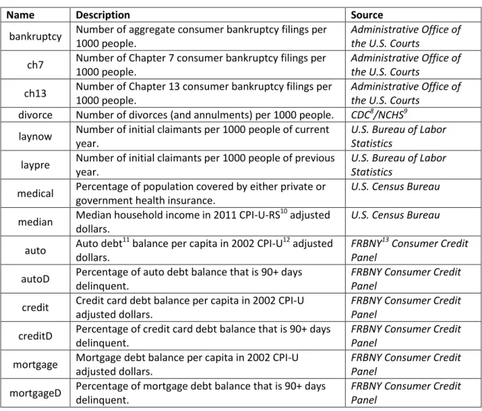
The sources of which the data is gathered from and a description of each variable can be seen in

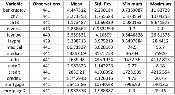
Table 1 overleaf. Each variable is then summarised further in Table 2. As can be seen in Table 2, most

the variables have all 441 observations (49states

x 9years). Laynow has only one observation missing

(Wyoming 2007) and laypre has only two observations missing (Wyoming 2001 and 2008). Although

divorce has a total of 28 missing observations, only five states lack at least one of their observations

for divorce.

7

The Centers for Disease Control & Prevention confirmed to me that, although money is

provided to states to collect data on marriage and divorce, many states have opted not to do so

because of the prohibitive cost.

5

Defined by the U.S. Bureau of Labor Statistics as “a person who files any notice of unemployment to initiate a

request either for a determination of entitlement to and eligibility for compensation, or for a subsequent

period of unemployment within a benefit year or period of eligibility” [http://www.bls.gov/bls/glossary.htm].

6

Based on estimates from the U.S. Census Bureau

[http://www.census.gov/popest/data/state/totals/2012/index.html].

7

_{The following observations are missing for divorce: Georgia (2004-2009), Hawaii (2003- 2009), Louisiana}

7

Table 1: Variable Descriptions and Sources

Name

Description

Source

bankruptcy

Number of aggregate consumer bankruptcy filings per

1000 people.

Administrative Office of

the U.S. Courts

ch7

Number of Chapter 7 consumer bankruptcy filings per

1000 people.

Administrative Office of

the U.S. Courts

ch13

Number of Chapter 13 consumer bankruptcy filings per

1000 people.

Administrative Office of

the U.S. Courts

divorce

Number of divorces (and annulments) per 1000 people.

CDC

8

/NCHS

9

laynow

Number of initial claimants per 1000 people of current

year.

U.S. Bureau of Labor

Statistics

laypre

Number of initial claimants per 1000 people of previous

year.

U.S. Bureau of Labor

Statistics

medical

Percentage of population covered by either private or

government health insurance.

U.S. Census Bureau

median

Median household income in 2011 CPI-U-RS

10

adjusted

dollars.

U.S. Census Bureau

auto

Auto debt

11

balance per capita in 2002 CPI-U

12

adjusted

dollars.

FRBNY

13

Consumer Credit

Panel

autoD

Percentage of auto debt balance that is 90+ days

delinquent.

FRBNY Consumer Credit

Panel

credit

Credit card debt balance per capita in 2002 CPI-U

adjusted dollars.

FRBNY Consumer Credit

Panel

creditD

Percentage of credit card debt balance that is 90+ days

delinquent.

FRBNY Consumer Credit

Panel

mortgage

Mortgage debt balance per capita in 2002 CPI-U

adjusted dollars.

FRBNY Consumer Credit

Panel

mortgageD

Percentage of mortgage debt balance that is 90+ days

delinquent.

FRBNY Consumer Credit

Panel

Note that the data extracted from the Administrative Office of the U.S. Courts for the variables bankruptcy, ch7 and ch13 were given originally as total filings. I converted the data so that it became the number of flings per 1000 people by using intercensal population estimates from the US Census Bureau. Furthermore, the variables auto, credit and mortgage were given by the FRBNY Consumer Credit Panel in nominal terms before being adjusted for inflation by using data from the US Inflation Calculator14.

One must point out that some academics doubt the accuracy of the bankruptcy data collected by the

Administrative Office of the U.S. Courts. The Administrative Office is responsible for recording the

official data on both business bankruptcy filings and consumer bankruptcy filings. From 1985 to

2005, business bankruptcies as a percentage of total bankruptcies (business and consumer)

monotonically decreased from 18.3% to 2.0%.

15

Lawless and Warren (2005) investigated this trend

8

_{Centers for Disease Control and Prevention}

9

National Center for Health Statistics

10

CPI Research Series Using Current Methods

11

Debt from an automobile loan (a personal loan used to purchase an automobile).

12

_{CPI for All Urban Consumers}

13

Federal Reserve Bank of New York

14

[http://www.usinflationcalculator.com/inflation/consumer-price-index-and-annual-percent-changes-from-1913-to-2008/]

15

8

by comparing the Administrative Office’s data on business bankruptcies against other measures of

business failures. The data on business failures from Dun and Bradstreet

16

were positively correlated

with the Administrative Office’s data on business bankruptcies up until 1985 but then, from 1986 to

1998, there existed a negative correlation between the two measures. Data from the Small Business

Administration

17

also suggested that the Administrative Office’s data was undercounting business

bankruptcies. Lawless and Warren concluded that since the mid-eighties, many business

bankruptcies were being filed as consumer bankruptcies instead.

It is claimed that “gray areas… are often part and parcel of smaller business bankruptcies” (Frasier,

1996, p.314) and so there is a prevalent error in identifying bankruptcy cases as business or

consumer. Nevertheless, one must accept that the data collected from the Administrative Office is

the official count of consumer bankruptcy filings and the best data we have. However, it is clear that

improvements can be made to the ways in which consumer bankruptcy data is collected and

processed in order to improve the accuracy and reliability of the data.

Table 2: Summary Statistics of Variables

Variable

Observations

Mean

Std. Dev.

Minimum

Maximum

bankruptcy

441

4.447512

2.290184

0.7369087

11.63729

ch7

441

3.271353

1.755688

0.373554

10.04255

ch13

441

1.173487

1.069339

0.080155

5.641573

divorce

413

3.888862

0.9622596

1.7

7.4

laynow

440

5.559831

4.20899

0.5448838

26.81376

laypre

439

5.208713

3.975219

0.5407684

28.4412

medical

441

86.71927

3.828163

74.5

95.7

median

441

53262.09

8131.258

36704

75920

auto

441

2689.98

496.1924

1432.56

4112.813

autoD

441

2.587823

1.143228

0.77

8.18

credit

441

2833.21

410.8392

1728.905

4216.554

creditD

441

8.742948

2.126016

4.73

20.75

mortgage

441

25413.86

10340.68

7995.92

54013.2

mortgageD

441

1.983878

1.988887

0.3

19.46

METHODOLOGY

Pooled ordinary least squares (OLS) estimation, fixed effects estimation and random effects

estimation will all be used to test the hypotheses made previously in the ‘Theoretical Framework’

section. It will then be decided as to which of these three econometric techniques gives the most

reliable inferences.

POOLED OLS

For the pooled OLS estimation, we will focus on the following model:

16

Dun & Bradstreet is a credit-reporting and business information firm. More details about the firm can be

found on their website [http://www.dnb.com/company.html].

17

_{The Small Business Administration is a U.S. government agency that assists small businesses. More details}

9

Notice that the dependent variable and the four independent variables we are interested in are

logged. This is done so that our inferences can be made in percentage terms rather than absolute

terms. Thus, it will enable us to see how a one percent change in the divorce rate, layoff rate and

medical insurance rate will affect the percentage change in the bankruptcy rate.

One important assumption of this model is that for any given values of the independent variables,

the expected error term is equal to zero. In other words, the error term must be uncorrelated with

each and every independent variable in the model (Barr, 2012). If there is a variable omitted from

the model which is correlated with both the dependent variable and one or more of the

independent variables then this assumption is violated and hence our inferences will no longer be

reliable. Thus, although we are only really interested in the coefficients of lndivorce, lnlaynow,

lnlaypre and lnmedical, seven other independent variables have been included in the model in order

to mitigate omitted variable bias.

We would expect a negative correlation between bankruptcy and the median household income as

we would expect a higher income would increase the likelihood of being able to repay debts.

Moreover, it is also highly likely that the amount of auto, credit card and mortgage debt affects

someone’s decision to file for bankruptcy. The proportion of auto, credit card and mortgage debt

that is delinquent will also be likely to be correlated with bankruptcy. Thus, the seven additional

regressors are all suspected to be correlated with the dependent variable. If they are also correlated

with at least one of lndivorce, lnlaynow, lnlaypre or lnmedical then they should be included in the

model.

Divorces are often caused by financial strain and all of the seven additional variables have an

influence on the financial stability of a household. We would also expect that current and previous

layoffs would be correlated with delinquent debt due to the loss of income from losing one’s job.

Furthermore, a higher income is likely to be positively correlated with being able to afford medical

insurance. This provides us with good reasoning to include median, auto, autoD, credit, creditD,

mortgage and mortgageD in our model so that we deal with the problem of endogeneity. The

10

suspected correlations have all been tested and the inclusion of all the independent variables in the

model is justified.

18

One major problem with using pooled OLS estimation with a panel dataset is that it is highly likely

that the model suffers from serial correlation. In other words, it is very likely that the error term in

one year is correlated to the error term in another year and so the estimated standard errors will

not reflect the true standard errors and this could lead to incorrect inferences.

FIXED EFFECTS

Fixed effects estimation is based on a model of time-demeaned variables. First, consider the

following equation:

Notice that in this equation the error term has been decomposed into two parts: the time-invariant

error term

that is common to all of the observations relating to a particular state; the

idiosyncratic error term

that varies across each state and across time even within a state (Barr,

2012). Next, note that in order to average a variable over time we apply the formula:

Now, consider the following equation of variables averaged over time:

A time-demeaned variable is given by the formula:

Thus, subtracting equation (2) from equation (1) will give us the fixed effects transformation of the

model:

We can see that the time-invariant error term is no longer included in the model after the fixed

effects transformation. Thus, in fixed effects estimation it does not matter if an independent

18

11

variable is correlated with the time-invariant error. One important assumption, however, is that for

any given values of the independent variables and the time-invariant error term, the expected

idiosyncratic error term must equal zero for each time period. Furthermore, there should be no

perfect linear relationship between the independent variables. The last two assumptions are

required (but not sufficient) to get unbiased estimates. We also require the idiosyncratic error term

to be homoscedastic. (Wooldridge, 2009)

A flaw of fixed effects estimation is that any time-invariant independent variable will not be included

in the model as time-demeaning it will make it equal to zero. Fortunately, all our independent

variables vary over time.

19

As previously mentioned, our data on divorce has missing observations.

However, for each state we have observations from at least two years which makes fixed effects

estimation feasible. Also, if “the reason we have missing data for some i is not correlated with the

idiosyncratic errors, the unbalanced panels cause no problems” (Wooldridge, 2009, p.488). As there

is no reason to believe that a state’s ability to afford data collection on divorce is correlated with our

idiosyncratic error term, the missing observations should cause no harm.

RANDOM EFFECTS

The third econometric technique used in this study is random effects estimation. The composite

error term (the aggregate of the idiosyncratic error term and the time-invariant error term) is used

in the model for random effects. As a result of the inclusion of the time-invariant error term in the

model, serial correlation will remain a problem. Random effects estimation overcomes this problem

by using generalised least squares (GLS) as opposed to the OLS used in the other two techniques

(Wooldridge, 2009). The GLS transformation of the model which is used in random effects

estimation is:

Each variable in the model has been partially-demeaned: enough to deal with the problem of serial

correlation but without throwing away too much variation. In this sense, random effects estimation

is more efficient than fixed effects estimation and thus leads to better inferences. However, unlike

fixed effects estimation, random effects estimation requires that the time-invariant error is

uncorrelated with all the independent variables and that it is homoscedastic. The value of λ in the

model is greater than zero and no larger than one. It can be shown that if λ were to equal zero, the

model would be the same as the pooled OLS model and if λ were to equal one, the model would be

the same as the fixed effects model. (Barr, 2009)

19

12

To summarise, pooled OLS estimation includes all of the time-invariant error in the model, random

effects estimation partially includes the time-invariant error in the model and fixed effects does not

include any of the time-invariant error in the model. Thus, it is useful to use all three techniques and

compare the three sets of estimates in order to analyse the bias caused by the inclusion of the

time-invariant error. Even if the time-time-invariant error term is uncorrelated with all the independent

variables in all the time periods, pooled OLS estimation still tends to suffer from serial correlation in

its error terms. Hence, fixed effects and random effects estimations give us more valid inferences.

The latter is preferred to the former as it is more efficient but only if the time-invariant errors are

uncorrelated with the independent variables. In order to choose which estimation to use, a

Hausman test will be carried out which looks at the sampling variation of the fixed effects estimates

and also compares the coefficients of the fixed effects and random effects estimates. (Wooldridge,

2009)

EMPIRICAL RESULTS

Table 4 gives an overview of all the regression results. STATA, the software used in this study, has

built-in features to control for heteroscedasticity in all three econometric techniques used.

20

However, even with homoscedasticity, pooled OLS estimation still suffers from serial correlation in

its error terms. Thus, our focus turns to fixed effects and random effects estimation and a Hausman

test is used to determine which of these estimations we will make our inferences from. The random

effects model is the more efficient of the two models and the fixed effects model the more

consistent. The Hausman test checks that the more efficient random effects model gives consistent

estimates by comparing it against the more consistent fixed effects model (Princeton University DSS,

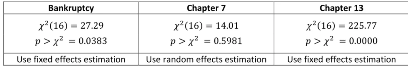
2003). The Hausman test was run for each of the three dependent variables and the results can be

seen in Table 3.

Table 3: Hausman Tests

Bankruptcy

Chapter 7

Chapter 13

Use fixed effects estimation

Use random effects estimation

Use fixed effects estimation

Interestingly, the Hausman test suggests using fixed effects estimation for bankruptcy and Chapter

13 but not Chapter 7. This suggests that there is some omitted time-invariant variable which is

correlated with Chapter 13 but not Chapter 7. Because of this omitted variable, random effects

estimation for bankruptcy and Chapter 13 will suffer from endogeneity. It can be speculated as to

what this time-invariant omitted variable is.

Prior to BAPCPA, the consumer could choose between Chapter 7 and Chapter 13 and so anything

which would affect the consumer’s decision to file for one chapter would inevitably affect his/her

decision to file under the other chapter. Hence, it is most likely that this omitted variable was

20

13

correlated with Chapter 13 and not Chapter 7 only after BAPCPA when consumers lost the privilege

to choose between the chapters: so a variable which affected the consumer’s decision to file for one

chapter no longer necessarily affected their decision to file for the other. As Chapter 13 was forced

on those who had incomes exceeding a certain threshold, this omitted variable should only affect

those with incomes above the threshold and not those below as then the omitted variable would

also influence Chapter 7 filings.

One supposition is that only those with relatively high incomes are affected by the stigma associated

with bankruptcy due to their social class and that this stigma varies across states but not over time.

Another theory is that recent college graduates have large student debts which makes them more

likely to file for bankruptcy. Since college graduates earn relatively high incomes, they will only be

eligible to file under Chapter 13 and not Chapter 7. However, for this conjecture to hold, the number

of recent college graduates per thousand will have to be time invariant which may not be the case.

Nevertheless, we will use the results from the Hausman test to select the results we will make our

inferences from as summarised in Table 5.

14

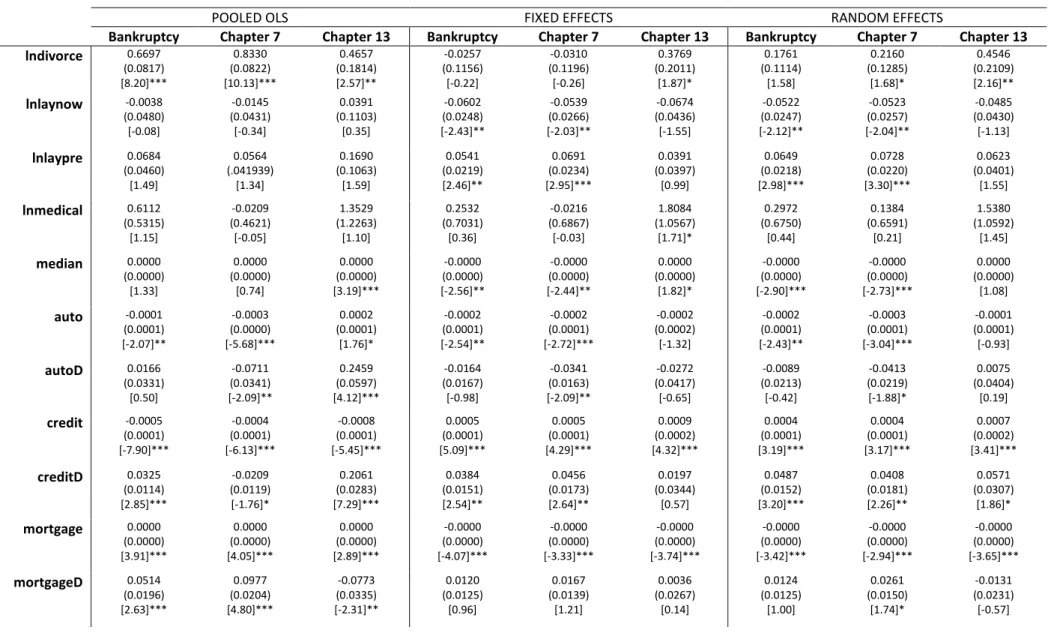
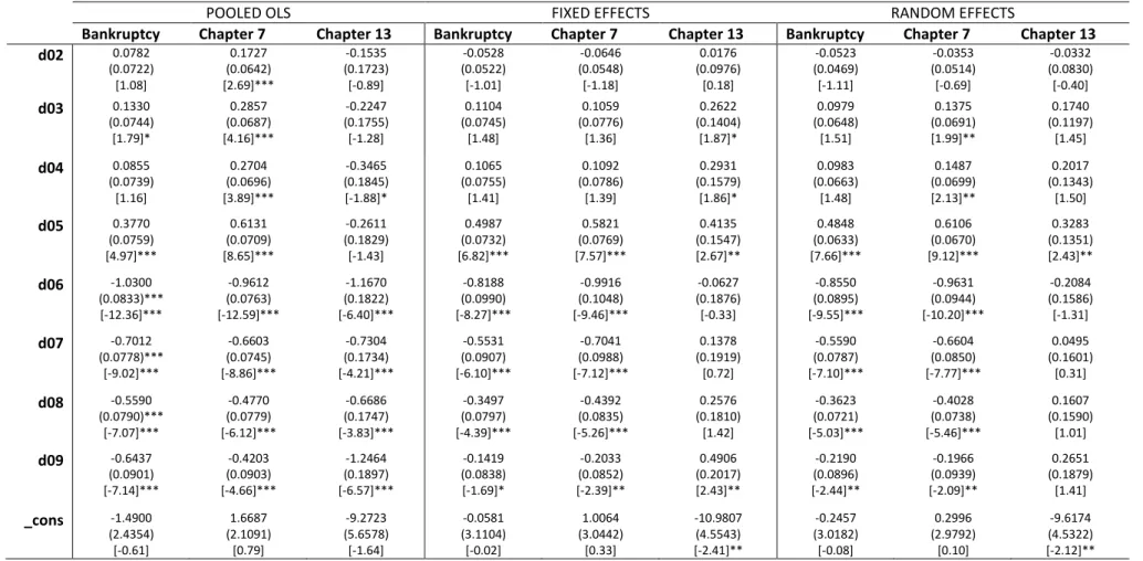
Table 4: Pooled OLS, Fixed Effects and Random Effects Regression Results

POOLED OLS

FIXED EFFECTS

RANDOM EFFECTS

Bankruptcy

Chapter 7

Chapter 13

Bankruptcy

Chapter 7

Chapter 13

Bankruptcy

Chapter 7

Chapter 13

lndivorce

0.6697 (0.0817) [8.20]*** 0.8330 (0.0822) [10.13]*** 0.4657 (0.1814) [2.57]** -0.0257 (0.1156) [-0.22] -0.0310 (0.1196) [-0.26] 0.3769 (0.2011) [1.87]* 0.1761 (0.1114) [1.58] 0.2160 (0.1285) [1.68]* 0.4546 (0.2109) [2.16]**

lnlaynow

-0.0038 (0.0480) [-0.08] -0.0145 (0.0431) [-0.34] 0.0391 (0.1103) [0.35] -0.0602 (0.0248) [-2.43]** -0.0539 (0.0266) [-2.03]** -0.0674 (0.0436) [-1.55] -0.0522 (0.0247) [-2.12]** -0.0523 (0.0257) [-2.04]** -0.0485 (0.0430) [-1.13]

lnlaypre

0.0684 (0.0460) [1.49] 0.0564 (.041939) [1.34] 0.1690 (0.1063) [1.59] 0.0541 (0.0219) [2.46]** 0.0691 (0.0234) [2.95]*** 0.0391 (0.0397) [0.99] 0.0649 (0.0218) [2.98]*** 0.0728 (0.0220) [3.30]*** 0.0623 (0.0401) [1.55]

lnmedical

0.6112 (0.5315) [1.15] -0.0209 (0.4621) [-0.05] 1.3529 (1.2263) [1.10] 0.2532 (0.7031) [0.36] -0.0216 (0.6867) [-0.03] 1.8084 (1.0567) [1.71]* 0.2972 (0.6750) [0.44] 0.1384 (0.6591) [0.21] 1.5380 (1.0592) [1.45]

median

0.0000 (0.0000) [1.33] 0.0000 (0.0000) [0.74] 0.0000 (0.0000) [3.19]*** -0.0000 (0.0000) [-2.56]** -0.0000 (0.0000) [-2.44]** 0.0000 (0.0000) [1.82]* -0.0000 (0.0000) [-2.90]*** -0.0000 (0.0000) [-2.73]*** 0.0000 (0.0000) [1.08]

auto

-0.0001 (0.0001) [-2.07]** -0.0003 (0.0000) [-5.68]*** 0.0002 (0.0001) [1.76]* -0.0002 (0.0001) [-2.54]** -0.0002 (0.0001) [-2.72]*** -0.0002 (0.0002) [-1.32] -0.0002 (0.0001) [-2.43]** -0.0003 (0.0001) [-3.04]*** -0.0001 (0.0001) [-0.93]

autoD

0.0166 (0.0331) [0.50] -0.0711 (0.0341) [-2.09]** 0.2459 (0.0597) [4.12]*** -0.0164 (0.0167) [-0.98] -0.0341 (0.0163) [-2.09]** -0.0272 (0.0417) [-0.65] -0.0089 (0.0213) [-0.42] -0.0413 (0.0219) [-1.88]* 0.0075 (0.0404) [0.19]

credit

-0.0005 (0.0001) [-7.90]*** -0.0004 (0.0001) [-6.13]*** -0.0008 (0.0001) [-5.45]*** 0.0005 (0.0001) [5.09]*** 0.0005 (0.0001) [4.29]*** 0.0009 (0.0002) [4.32]*** 0.0004 (0.0001) [3.19]*** 0.0004 (0.0001) [3.17]*** 0.0007 (0.0002) [3.41]***

creditD

0.0325 (0.0114) [2.85]*** -0.0209 (0.0119) [-1.76]* 0.2061 (0.0283) [7.29]*** 0.0384 (0.0151) [2.54]** 0.0456 (0.0173) [2.64]** 0.0197 (0.0344) [0.57] 0.0487 (0.0152) [3.20]*** 0.0408 (0.0181) [2.26]** 0.0571 (0.0307) [1.86]*

mortgage

0.0000 (0.0000) [3.91]*** 0.0000 (0.0000) [4.05]*** 0.0000 (0.0000) [2.89]*** -0.0000 (0.0000) [-4.07]*** -0.0000 (0.0000) [-3.33]*** -0.0000 (0.0000) [-3.74]*** -0.0000 (0.0000) [-3.42]*** -0.0000 (0.0000) [-2.94]*** -0.0000 (0.0000) [-3.65]***

mortgageD

0.0514 (0.0196) [2.63]*** 0.0977 (0.0204) [4.80]*** -0.0773 (0.0335) [-2.31]** 0.0120 (0.0125) [0.96] 0.0167 (0.0139) [1.21] 0.0036 (0.0267) [0.14] 0.0124 (0.0125) [1.00] 0.0261 (0.0150) [1.74]* -0.0131 (0.0231) [-0.57]

15

Table 4 Continued

POOLED OLS

FIXED EFFECTS

RANDOM EFFECTS

Bankruptcy

Chapter 7

Chapter 13

Bankruptcy

Chapter 7

Chapter 13

Bankruptcy

Chapter 7

Chapter 13

d02

0.0782 (0.0722) [1.08] 0.1727 (0.0642) [2.69]*** -0.1535 (0.1723) [-0.89] -0.0528 (0.0522) [-1.01] -0.0646 (0.0548) [-1.18] 0.0176 (0.0976) [0.18] -0.0523 (0.0469) [-1.11] -0.0353 (0.0514) [-0.69] -0.0332 (0.0830) [-0.40]

d03

0.1330 (0.0744) [1.79]* 0.2857 (0.0687) [4.16]*** -0.2247 (0.1755) [-1.28] 0.1104 (0.0745) [1.48] 0.1059 (0.0776) [1.36] 0.2622 (0.1404) [1.87]* 0.0979 (0.0648) [1.51] 0.1375 (0.0691) [1.99]** 0.1740 (0.1197) [1.45]

d04

0.0855 (0.0739) [1.16] 0.2704 (0.0696) [3.89]*** -0.3465 (0.1845) [-1.88]* 0.1065 (0.0755) [1.41] 0.1092 (0.0786) [1.39] 0.2931 (0.1579) [1.86]* 0.0983 (0.0663) [1.48] 0.1487 (0.0699) [2.13]** 0.2017 (0.1343) [1.50]

d05

0.3770 (0.0759) [4.97]*** 0.6131 (0.0709) [8.65]*** -0.2611 (0.1829) [-1.43] 0.4987 (0.0732) [6.82]*** 0.5821 (0.0769) [7.57]*** 0.4135 (0.1547) [2.67]** 0.4848 (0.0633) [7.66]*** 0.6106 (0.0670) [9.12]*** 0.3283 (0.1351) [2.43]**

d06

-1.0300 (0.0833)*** [-12.36]*** -0.9612 (0.0763) [-12.59]*** -1.1670 (0.1822) [-6.40]*** -0.8188 (0.0990) [-8.27]*** -0.9916 (0.1048) [-9.46]*** -0.0627 (0.1876) [-0.33] -0.8550 (0.0895) [-9.55]*** -0.9631 (0.0944) [-10.20]*** -0.2084 (0.1586) [-1.31]

d07

-0.7012 (0.0778)*** [-9.02]*** -0.6603 (0.0745) [-8.86]*** -0.7304 (0.1734) [-4.21]*** -0.5531 (0.0907) [-6.10]*** -0.7041 (0.0988) [-7.12]*** 0.1378 (0.1919) [0.72] -0.5590 (0.0787) [-7.10]*** -0.6604 (0.0850) [-7.77]*** 0.0495 (0.1601) [0.31]

d08

-0.5590 (0.0790)*** [-7.07]*** -0.4770 (0.0779) [-6.12]*** -0.6686 (0.1747) [-3.83]*** -0.3497 (0.0797) [-4.39]*** -0.4392 (0.0835) [-5.26]*** 0.2576 (0.1810) [1.42] -0.3623 (0.0721) [-5.03]*** -0.4028 (0.0738) [-5.46]*** 0.1607 (0.1590) [1.01]

d09

-0.6437 (0.0901) [-7.14]*** -0.4203 (0.0903) [-4.66]*** -1.2464 (0.1897) [-6.57]*** -0.1419 (0.0838) [-1.69]* -0.2033 (0.0852) [-2.39]** 0.4906 (0.2017) [2.43]** -0.2190 (0.0896) [-2.44]** -0.1966 (0.0939) [-2.09]** 0.2651 (0.1879) [1.41]

_cons

-1.4900 (2.4354) [-0.61] 1.6687 (2.1091) [0.79] -9.2723 (5.6578) [-1.64] -0.0581 (3.1104) [-0.02] 1.0064 (3.0442) [0.33] -10.9807 (4.5543) [-2.41]** -0.2457 (3.0182) [-0.08] 0.2996 (2.9792) [0.10] -9.6174 (4.5322) [-2.12]**

Results are shown in the format: Coefficient, (Cluster Robust Standard Error), [t-statistic / z-statistic]. *Significant at the 10% level **Significant at the 5% level ***Significant at the 1% level

16

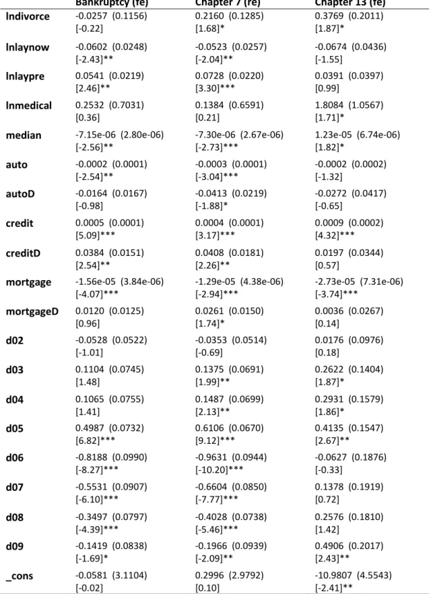
Table 5: Main Results

Bankruptcy (fe)

Chapter 7 (re)

Chapter 13 (fe)

lndivorce

-0.0257 (0.1156)

[-0.22]

0.2160 (0.1285)

[1.68]*

0.3769 (0.2011)

[1.87]*

lnlaynow

-0.0602 (0.0248)

[-2.43]**

-0.0523 (0.0257)

[-2.04]**

-0.0674 (0.0436)

[-1.55]

lnlaypre

0.0541 (0.0219)

[2.46]**

0.0728 (0.0220)

[3.30]***

0.0391 (0.0397)

[0.99]

lnmedical

0.2532 (0.7031)

[0.36]

0.1384 (0.6591)

[0.21]

1.8084 (1.0567)

[1.71]*

median

-7.15e-06 (2.80e-06)

[-2.56]**

-7.30e-06 (2.67e-06)

[-2.73]***

1.23e-05 (6.74e-06)

[1.82]*

auto

-0.0002 (0.0001)

[-2.54]**

-0.0003 (0.0001)

[-3.04]***

-0.0002 (0.0002)

[-1.32]

autoD

-0.0164 (0.0167)

[-0.98]

-0.0413 (0.0219)

[-1.88]*

-0.0272 (0.0417)

[-0.65]

credit

0.0005 (0.0001)

[5.09]***

0.0004 (0.0001)

[3.17]***

0.0009 (0.0002)

[4.32]***

creditD

0.0384 (0.0151)

[2.54]**

0.0408 (0.0181)

[2.26]**

0.0197 (0.0344)

[0.57]

mortgage

-1.56e-05 (3.84e-06)

[-4.07]***

-1.29e-05 (4.38e-06)

[-2.94]***

-2.73e-05 (7.31e-06)

[-3.74]***

mortgageD

0.0120 (0.0125)

[0.96]

0.0261 (0.0150)

[1.74]*

0.0036 (0.0267)

[0.14]

d02

-0.0528 (0.0522)

[-1.01]

-0.0353 (0.0514)

[-0.69]

0.0176 (0.0976)

[0.18]

d03

0.1104 (0.0745)

[1.48]

0.1375 (0.0691)

[1.99]**

0.2622 (0.1404)

[1.87]*

d04

0.1065 (0.0755)

[1.41]

0.1487 (0.0699)

[2.13]**

0.2931 (0.1579)

[1.86]*

d05

0.4987 (0.0732)

[6.82]***

0.6106 (0.0670)

[9.12]***

0.4135 (0.1547)

[2.67]**

d06

-0.8188 (0.0990)

[-8.27]***

-0.9631 (0.0944)

[-10.20]***

-0.0627 (0.1876)

[-0.33]

d07

-0.5531 (0.0907)

[-6.10]***

-0.6604 (0.0850)

[-7.77]***

0.1378 (0.1919)

[0.72]

d08

-0.3497 (0.0797)

[-4.39]***

-0.4028 (0.0738)

[-5.46]***

0.2576 (0.1810)

[1.42]

d09

-0.1419 (0.0838)

[-1.69]*

-0.1966 (0.0939)

[-2.09]**

0.4906 (0.2017)

[2.43]**

_cons

-0.0581 (3.1104)

[-0.02]

0.2996 (2.9792)

[0.10]

-10.9807 (4.5543)

[-2.41]**

Results are shown in the format: Coefficient, (Cluster Robust Standard Error), [t-statistic / z-statistic]. *Significant at the 10% level **Significant at the 5% level ***Significant at the 1% level

Note that the t-statistics and z-statistics have been rounded to two decimal places and the coefficients and standard errors to four decimal places except in the case where this gives zero where it is instead rounded to three significant figures.

17

In regard to the first hypothesis, it seems that there is no significant relationship between the

divorce rate and the aggregate bankruptcy rate. However, a positive relationship exists between the

divorce rate and both the Chapter 7 rate and the Chapter 13 rate, albeit only at the 10% significance

level. A 1% increase in the divorce rate is associated with a 0.22% increase in the Chapter 7 rate and

a 0.38% increase in the Chapter 13 rate. Although these results are not overwhelming, they confirm

that divorce does in fact influence bankruptcy.

Significant results are also found regarding layoffs and their effect on the aggregate bankruptcy rate

and the Chapter 7 rate but not the Chapter 13 rate. The number of layoffs in the same calendar year

(laynow) measures the contemporaneous effect of being laid off and the number of layoffs in the

previous calendar year (laypre) measures the delayed effect of being laid off. It makes sense that

layoffs do not affect Chapter 13 bankruptcies as consumers would have been less likely to have a job

when filing and so could not engage in a repayment plan. As expected, the relationship between

lagged layoffs and bankruptcy is positive: a 1% increase in the previous year’s layoff rate is

associated with a 0.05% increase in the bankruptcy rate and a 0.07% increase in the Chapter 7 rate.

On the other hand, the relationship between instant layoffs and bankruptcy was significant and

surprisingly negative: a 1% increase in the current year’s layoff rate is associated with a 0.06% fall in

the bankruptcy rate and a 0.05% decrease in the Chapter 7 rate. After BAPCPA, the consumer’s

income was measured based on his/her average income over the six months prior to filing. This

income would then determine whether he/she exceeded the threshold to file under the more

favourable Chapter 7. Thus, it may have been that those who were laid off purposely delayed filing

so that their measured income would be lower.

Perhaps the most disappointing result with respect to the three hypotheses is on health insurance.

The signs on the coefficients on health insurance are positive for bankruptcy, Chapter 7 and Chapter

13, though only significantly for the latter. A 1% increase in the proportion of the population with

health insurance is associated with a 0.25% increase in the bankruptcy rate and a 1.81% rise in the

Chapter 13 rate. This unanticipated result may be due to the percentage of people with health

insurance being a poor indicator of the impact of facing unexpected medical costs. Firstly, the quality

of health insurance may differ between insurance provided by employment, insurance purchased

directly and insurance provided by the government. Furthermore, even those who are insured at the

time of illness may still face additional out-of pocket costs (Himmelstein et al, 2005). In hindsight, a

better variable to use would have been out of insurance medical costs; though such data is

unavailable on a state-level.

Most of the control variables turned out as expected. An increase in the real household income of

$1,000 (in 2011 dollars) is associated with a 0.72% decrease in the bankruptcy rate, driven mainly by

its negative impact on the Chapter 7 rate. A significant positive relationship holds between the

bankruptcy rate and credit card debt and credit card delinquency: a real $100 increase (in 2002

dollars) increases the bankruptcy rate by 5%; a one percentage point increase in the percentage of

credit card debt that is delinquent increases the bankruptcy rate by 3.84%. Mortgage and auto debt

have a significant negative relationship with the bankruptcy rate, possibly because the largest loans

go to those with the best credit rating. The percentage of mortgage debt and auto debt delinquent

was only significant for Chapter 7 and only at the 10% significance level. However, for auto debt

delinquency the coefficients are surprisingly negative.

18

As anticipated, the 2005 year dummy was positive and highly significant as, for the first ten months,

consumers rushed to file for bankruptcy before the more stringent laws of BAPCPA were in place. In

the years that followed, the bankruptcy rate declined as a result of the less debtor-friendly litigation.

Table 6 shows the results of testing consecutive dummy variables against each other to confirm their

significance.

Table 6: Testing Dummy Variables

test d04=d05

test d05=d06

test d06=d07

test d07=d08

test d08=d09

Bankruptcy

Chapter 7

Chapter 13

Moreover, regressions were run to see if the impact of divorce, layoffs and medical insurance

changed over time.

21

From 2002-2008, the positive relationship between the divorce rate and the

Chapter 13 rate fell significantly. Given the timescale, this change was not due to BAPCPA and it is

unclear as to why exactly this is the case. However, the relationship of the current and previous

year’s layoff rate with both the bankruptcy rate and the Chapter 7 rate became more positive in the

three calendar years after BAPCPA. This may be because BAPCPA eliminated the impact of

consumers filing tactically to maximise their financial gains which made the impact of adverse effects

like layoffs more influential in dictating the bankruptcy rate. The relationship between health

insurance and the bankruptcy rate also became significantly more positive from 2006 to 2009,

supporting this hypothesis.

CONCLUSION

This study has found that the adverse effects of divorce and job loss are indeed determinants of

bankruptcy. If the divorce rate rises by 1% then the Chapter 7 bankruptcy rate and Chapter 13

bankruptcy rate increase by 0.22% and 0.38% respectively. Moreover, the lagged effect of the layoff

rate has a significant positive relationship with the rate of bankruptcy: a 1% increase in the former

leads to a 0.05% rise to the latter. However, the contemporaneous effect of layoffs on bankruptcy

was significantly negative, suggesting that some filers may have purposely chosen not to file for

bankruptcy immediately after losing their jobs in order to lower their perceived income and become

eligible for Chapter 7 filing.

Furthermore, having health insurance was shown to not have any real impact on the bankruptcy rate

which may suggest that the adverse effect of high medical costs does not influence bankruptcy.

However, it may be that having health insurance does not stop one from facing unexpected medical

costs and so the relationship between this adverse effect and bankruptcy may in fact exist. Hence,

21

19

this study could have been improved by using a better measure of unforeseen medical costs.

Moreover, other variables could have been included in our models to deal with endogeneity such as

the number of subprime mortgages, casino gambling expenditure, a measure of social stigma and a

measure of the level of asset exemptions in each state.

It must also be pointed out that the Administrative Office of the US Courts ought to rethink the way

in which their data is collected as it is used to shape bankruptcy policy which not only affects the

credit industry but millions of ordinary people every year. Such data inaccuracies can undermine the

reliability of the academic studies which try to unravel the determinants of bankruptcy.

20

BIBLIOGRAPHY

Academic Publications:

Daraban, B. & Thies, C.F. (2010). “Estimating the Effects of Casinos and of Lotteries on Bankruptcy: A

Panel Data Set Approach”,

Journal of Gambling Studies

, Vol. 27, pp. 145-154

Domowitz, I. & Sartain, R.L. (1999). “Determinants of the Consumer Bankruptcy Decision”,

Journal of

Finance

, Vol. 54(1), pp. 403–420

Dranove, D. & Millenson, M.L. (2006). “Medical Bankruptcy: Myth versus Fact”,

Health Affairs

, Vol.

25(2), pp. 74-83

Fay, S., Hurst, E. & White, M.J. (2002). “The Household Bankruptcy Decision”,

American Economic

Review

, Vol. 92(3), pp. 706-718

Frasier, J.C. (1996). “Caught in a Cycle of Neglect: the Accuracy of Bankruptcy Statistics”,

101 COM.

L.J.

307-356

Gross, D.B. & Souleles, N.S. (2002). “An Empirical Analysis of Personal Bankruptcy and Delinquency”,

The Review of Financial Studies

, Vol. 15(1), pp. 319-347

Himmelstein, D.U., Warren, E., Thorne, D. & Woolhandler, S. (2005). “Illness and Injury as

Contributors to Bankruptcy,”

Health Affairs

, Vol. 24, pp. 63-73

Laibson, D., Repetto, A. & Tobacman, J. (2000). “A Debt Puzzle”,

NBER Working Paper

No. 7879

Lawless, R.M. & Warren, E. (2005). “The Myth of the Disappearing Business Bankruptcy”,

California

Law Review

, Vol. 93(3), pp. 1-52

Sullivan, T., Elizabeth W. & Westbrook, J.L. (2000). "The Fragile Middle Class: Americans in Debt

”,

Yale University Press

White, M.J. (2007). “Bankruptcy Reform and Credit Cards",

NBER Working Paper

No. 13265

Lectures:

Barr, A. (2012). “Simple and Multiple Regression Models: A review – Lecture 1”,

L13520

Econometrics Project

, University of Nottingham

Barr, A. (2012). “Panel data analysis (continued) - Lecture 5”,

L13520 Econometrics Project

,

University of Nottingham

Barr, A. (2012). “Panel data analysis (continued) - Lecture 7”,

L13520 Econometrics Project

,

University of Nottingham

21

Texts:

Wooldridge, J.M. (2009). “Introductory Econometrics: A Modern Approach”, 4

th

edition,

South-Western Cengage Learning

Websites:

Egan, T. (2005). “Newly Bankrupt Raking in Piles of Credit Offers”

, The New York Times

,

[URL:http://www.nytimes.com/2005/12/11/national/11credit.html]

Unknown author (2011), “Top 20 Celebrities who have Filed Bankruptcy”,

How to Save Money

,

[URL:http://www.howtosavemoney.com/top-20-celebrities-who-have-filed-bankruptcy/#.UWswO8q0rDt]

Unknown author (2007), “Bankruptcy Law & Legal Definition”,

US Legal

,

[URL:http://definitions.uslegal.com/b/bankruptcy/]

Unknown author (2003), “Panel Data”,

Princeton University: Data and Statistical Services

,

[URL:http://dss.princeton.edu/online_help/stats_packages/stata/panel.htm]

22

APPENDIX

DATA

The monotonic decrease of business bankruptcies as a percentage of total bankruptcies (15

th

footnote)

The data is extracted from the Administrative Office of the US courts. The chart shows business bankruptcies

as a percentage of total bankruptcies from 1985 to 2005 for the twelve months ending June 30

th

.

METHODOLOGY

Variable Correlations (18

th

footnote)

median

auto

autoD

credit

creditD

mortgage mortgageD

lnbankruptcy

-0.2755

_0.0000

-0.0694

_0.1456

0.0456

_0.3390

-0.2941

_0.0000

0.1203

_0.0115

-0.3218

_0.0000

0.0337

_0.4804

lnch7

-0.1632

_0.0006

-0.1824

_0.0001

-0.1279

_0.0072

-0.1943

_0.0000

-0.0693

_0.1461

-0.2875

_0.0000

-0.0199

_0.6775

lnch13

-0.2288

_0.0000

0.1503

_0.0015

0.3528

_0.0000

-0.2448

_0.0000

0.4184

_0.0000

-0.1021

_0.0321

0.1731

_0.0003

median

auto

autoD

credit

creditD

mortgage mortgageD

lndivorce

-0.3391

_0.0000

0.3741

_0.0000

0.0190

_0.7009

-0.1988

_0.0000

0.1884

_0.0001

-0.2553

_0.0000

0.0104

_0.8331

lnlaynow

-0.0542

_0.2568

-0.3366

_0.0000

0.0620

_0.1942

-0.1698

_0.0003

0.0730

_0.1261

-0.1725

_0.0003

0.1790

_0.0002

lnlaypre

-0.0470

_0.3260

-0.2640

_0.0000

-0.0463

_0.3329

-0.1495

_0.0017

0.0561

_0.2406

-0.1882

_0.0001

0.0421

_0.3789

lnmedical

0.4291

_0.0000

-0.5532

_0.0000

-0.3686

_0.0000

0.1054

_0.0268

-0.5161

_0.0000

0.1086

_0.0226

-0.2289

_0.0000

0%

2%

4%

6%

8%

10%

12%

14%

16%

18%

20%

23

All the independent variables are time variant (19

th

footnote)

lndivorce

The year. | Mean Std. Dev. Freq. ---+--- 2001 | 1.3932599 .22386326 47 2002 | 1.3730467 .23991981 48 2003 | 1.3425108 .24828831 47 2004 | 1.3256608 .25311863 46 2005 | 1.3148767 .27552644 45 2006 | 1.325478 .25056263 45 2007 | 1.296886 .25589809 45 2008 | 1.2902984 .2357329 45 2009 | 1.2827669 .23777189 45 ---+--- Total | 1.3279216 .24712652 413

lnlaynow

The year. | Mean Std. Dev. Freq. ---+--- 2001 | 1.6968521 .81719092 49 2002 | 1.6087341 .68760678 49 2003 | 1.4043572 .72394347 49 2004 | 1.2123494 .66100363 49 2005 | 1.3181398 .80942862 49 2006 | 1.1426568 .75351402 49 2007 | 1.2290186 .72035576 48 2008 | 1.5023577 .7791332 49 2009 | 1.877504 .62307188 49

lnlaypre

The year. | Mean Std. Dev. Freq. ---+--- 2001 | 1.3331428 .786729 48 2002 | 1.6881956 .81745231 49 2003 | 1.6007746 .68784772 49 2004 | 1.3951641 .72500696 49 2005 | 1.2033423 .66232632 49 2006 | 1.3087209 .81511075 49 2007 | 1.1323886 .75656346 49 2008 | 1.220019 .72250562 48 2009 | 1.4939056 .78142718 49

lnmedical

The year. | Mean Std. Dev. Freq. ---+--- 2001 | 4.4764623 .04245643 49 2002 | 4.4685877 .04210686 49 2003 | 4.4599336 .04407133 49 2004 | 4.4638421 .03939533 49 2005 | 4.4607498 .04196299 49 2006 | 4.452912 .04918319 49 2007 | 4.4626107 .04688293 49 2008 | 4.4599233 .047009 49 2009 | 4.4501438 .04732838 49