MULTI-CHROMATIC ANALYSIS OF INSAR DATA: VALIDATION AND POTENTIAL

MULTI-CHROMATIC ANALYSIS OF INSAR DATA: VALIDATION AND POTENTIAL

Fabio Bovenga(1)_{, Vito Martino Giacovazzo}(1)_{, Alberto Refice}(1)_{, Nicola Veneziani}(1)_{, Raffaele Vitulli}(2)

(1)

CNR ISSIA, Bari, Via Amendola, 122/d - 70126 Bari (Italy), tel/fax +39 080 5929425 / 60 E-mail: [email protected]

(2)

ESA - ESTEC TEC/EDP, Noordwijk, The Netherlands, E-mail: [email protected]

ABSTRACT

The present paper presents the results of the application of Multi Chromatic Analysis (MCA) for height retrieval by processing both AES-1 airborne data and satellite TerraSAR-X data. In particular, a test of the robustness of the MCA technique with respect to total processed bandwidth has been performed through comparison of results from datasets with bandwidths spanning form 100 to 400 MHz.

A first validation of the mentioned technique has been carried out by comparing the retrieved heights w.r.t. ground elevation from external SRTM DEM, as well as by verifying the reliability of the fringe classifications based on the integer number of phase cycles computed through MCA.

Results are presented and commented by addressing potential and limitation of the technique.

1. INTRODUCTION

The Multi-Chromatic Analysis, as introduced in [1], uses interferometric pairs of SAR images processed at range sub-bands and explores the phase trend of each pixel as a function of the different central carrier frequencies. The phase of suitable “frequency-coherent” scatterers evolves linearly with the sub-band central wavelength, the slope being proportional to the absolute optical path difference. Unlike the conventional “monochromatic” InSAR approach, this new multi-chromatic technique allows performing spatially independent and absolute topographic measurements, if the attention is focused on single targets exhibiting stable phase behaviour across the frequency domain. These can be used to retrieve unambiguous height information, without the need for a spatial phase unwrapping process. Applying the same sub-band splitting to a single SAR image, the phase will also vary linearly with wavelength, the slope being proportional to the whole absolute optical path for the scattering center under concern. Potential applications for the study of frequency-stable targets include topographic measurements, atmospheric research, and urban monitoring.

Previous work on the subject has started demonstrating the practical feasibility of the technique by using simulations [1] as well as a set of SAR data collected by the airborne AES-1 radar interferometer, operating at X-band by multi-channel electronics, which provides a

total radar bandwidth of 400 MHz [2]. The technique appears optimally suited for the new generation of satellite sensors, which operate with larger bandwidths than those of previously available instruments, generally limited to about 20 MHz.

In the following, we briefly review the MCA mathematical formulation as well as some implementation aspects. A parametric analysis provides a first evaluation of the impact of the MCA processing parameters on the height estimation performances. Then, the application of the technique to Level 1 TerraSAR-X data is described, as well as to AES-1 airborne data acquired over an area of gently rolling topography, sited in the west-central part of Switzerland close to the village of Langnau. Results of the validation experiment are presented and commented.

2. MCA FORMULATION

To perform MCA in InSAR configuration, Ni sub-look images,{IM,i , IS,i} with i = 1, ..., Ni are generated for both master and slave views with the same parameters. Then, a set of Ni interferometric phase fields can be generated by cross-multiplying the master and slave sub-look images relative to the same central frequency fi, with phases:

i i i Rx r f c f r x =− ⋅∆ ⋅ =− ⋅∆ ⋅ Φ ( , ) 2π τ 4π ( , ) (1)

where ∆R = RM(x, r) − RS(x, r) and (x, r) are the azimuth and range pixel coordinates, respectively. Since only wrapped phase values are measured, the following relations hold: ) , ( 2 ) , ( ) , (xr W xr k xr i i =Φ + ⋅ Φ π i i W i f r x C r x C f r x R c r x k r x ⋅ + = = ⋅ ∆ ⋅ − ⋅ − = Φ ) , ( ) , ( ) , ( 4 ) , ( 2 ) , ( 1 0 π π ₍₂₎

This means that by exploring the trend of the wrapped interferometric phase values along frequencies, the range difference between master and slave can be inferred, which in turn is related to the elevation of the pixel: ) , ( 4 ) , (xr c C₁ xr R =− ⋅ ∆ π (3)

Moreover, the coefficient, C0(x, r), gives the integer number of 2π cycles that has to be added to the wrapped interferometric phase of the pixel (x, r) in order to infer its absolute value:

_____________________________________________________ Proc. ‘Fringe 2009 Workshop’, Frascati, Italy,

π 2 ) , ( ) , (_xr C0 x r k =− . (4)

This parameter allows to classify the fringes and to assign to each class the proper value to compute the absolute phase. Therefore, once the set of interferometric phase fields has been generated, the following processing step is a point-wise estimation of C0 and C1 through linear regression.

An a posteriori estimation of the multi-frequency phase error is given by the root mean square difference between the interferometric phases measured at the different frequencies fi, and the corresponding values computed by the linear model:

∑

[

( )

( )

( )

]

As in the monochromatic approach, where the coherence constitutes the quality factor for the measures, in the same way the quantity in (5), evaluated on a pixel-by-pixel basis, defines an inherent inter-band coherence for the MCA and can be assumed as a quality index of the measurements: the smaller σΦ, the better is the achievable accuracy for terrain heights. Hence the last processing step consists in selecting those pixels (targets) whose inter-band phase STD is below a reliability threshold: PSfd = {(x, r) | σΦ(x, r) ≤ σthΦ}. The statistical distribution of the k(x, r) values can also be exploited, in order to decrease the error of the point-wise estimates.

To validate the MCA, the absolute height values measured through relation (3) on selected pixels (PSfd) can be performed based on an external DEM. This step aims at assessing the accuracy of the multi-chromatic topographic phase and evaluating the importance of atmospheric delays, if present.

3. IMPLEMENTAITION ASPECTS

To perform MCA in InSAR configuration, for each selected frequency, a pair of master and slave sub-view images have to be generated and coregistered to a reference geometry: {SLCM,i , SLCS,i} with i = 1, ..., Ni. The first processing steps are band-splitting and coregistration.

Previous works and activities relative to MCA started demonstrating the practical feasibility of the technique by focusing raw SAR data to generate the sub-look images. However, the technique appears optimally suited for the new generation of satellite sensors, which operate with larger bandwidths than those of previously available instruments, generally limited to about 20 MHz. SAR sensors such as those mounted on TerraSAR-X or COSMO-SkyMed spacecraft, all pose great expectations on the potential use of multi-chromatic methods, but data policies of these missions do not foresee the delivery of raw data thus imposing to perform MCA starting from SLC images. In [2] the

equivalence between MCA performed starting from Level 0 and Level 1 data has been proved. The standard processors for Level 1 data production are considered as linear and phase preserving and all information in the frequency space is theoretically preserved except for Hamming filtering at the end of the focusing process. In order to avoid asymmetry in the spectrum, before the pass-band filtering a de-Hamming filter is required along range (see [2] for more details).

Concerning coregistration, in order to save processing time, it can be performed once between full-band images before sub-looks generation instead of Nf-times after band-splitting. In this configuration, the sub-band filtering performed after coregistration induces a further phase term related to the shift of range pixel, shr, applied to the slave image in order to be resampled onto the master geometry. According to this effect the interferometric phase becomes:

(

)

i R p R p f

c

p =− ⋅ ∆ −∆ ⋅

Φ ( ) 4π ( ) ( ) (6)

where ∆Rsh = dr ⋅ shr and dr is the pixel spacing. Thus, in order to infer ∆R through (3), it is necessary to take into account this term related to the coregistration range shift. This phase compensation is a trivial and not computationally expensive task compared with that required to perform coregistration for every sub-look. The range shift matrix shr(p) is already available as side product of the coregistration step. It is worthwhile to point out that ∆Rsh(p) represents a coarse estimation of the path difference between master and slave based on the amplitude cross-correlation, similar to what is done through radargrammetric techniques by using very large parallax values [3].

Once C1 is available through MCA, the height H(p) w.r.t. to a reference ellipsoid can be computed as (from [4], eqs. 3 and 6): p p p M B R p r p C c p H , , 1 ) sin( ) ( ) ( 4 ) ( ⊥ ⋅ ⋅ ⎥⎦ ⎤ ⎢⎣ ⎡ _{⋅ −} − = ref ϑ δ π (7)

where δr = ∆Rsh(p) −∆Rref(p), RM,p and θpref are respectively the range distance and the look angle relative to the master view computed w.r.t. the reference ellipsoid height at the pixel p, Bs is the geometrical distance (baseline) between the two acquisitions, B⊥,p is the component of the baseline orthogonal to the slant direction of the master computed at pixel p, the angle α defines the orientation of the baseline and, ∆Rref(p) is the absolute path difference computed w.r.t. the height of the reference ellipsoid at the pixel p. All these geometrical parameters vary on a pixel-by-pixel basis according to the sensor coordinates, and are known from InSAR pre-processing.

To perform validation we used a Digital Elevation Model (DEM) provided by the SRTM mission, which has been back-projected onto SAR geometry. Finally, we can observe that the matrix δr provides a very rough estimation of the height w.r.t. the reference ellipsoid.

Therefore, in Eq. (7) MCA contributes, through the C1 coefficient, to refine this coarse height model based on amplitude correlation.

4. PARAMETRIC ANALYSIS

A parametric analysis has been carried out with the aim of evaluating the impact of the MCA processing parameters on height estimation performance. By applying error propagation theory to the LMS linear regression, and assuming the same phase variance for all the sub-looks interferograms, σΦ = σΦi ∀i = 1, …, Nf , the STD for the coefficients C0 and C1 is:

( ) ( ) ( ) Φ = = = Φ = = ⎟ ⎟ ⎠ ⎞ ⎜ ⎜ ⎝ ⎛ − = ⎟ ⎟ ⎠ ⎞ ⎜ ⎜ ⎝ ⎛ − =

∑

∑

∑

∑

∑

The parameters involved in this analysis are in particular the number of sub-looks Nf, the sub-looks bandwidth Bp, and the full bandwidth B. Once fixed B and Bp, the maximum frequency range spanned by MCA is Be = B − Bp. The set of frequencies {fi} depends of Nf and df, which is the spectral distance between adjacent sub-looks. In order to model the σΦ dependency on Bp and to evaluate the behavior of the above relationships, we consider the favorable case of a scatterer which is an ideal metallic planar reflector, thus showing high Signal to Clutter Ratio (SRC). In this hypothesis the following relationships hold [5], [6]: clutter A A SCR SCR 0 2 2 4 , 2 1 σλ π σ = ⋅ ⋅ = Φ (8)

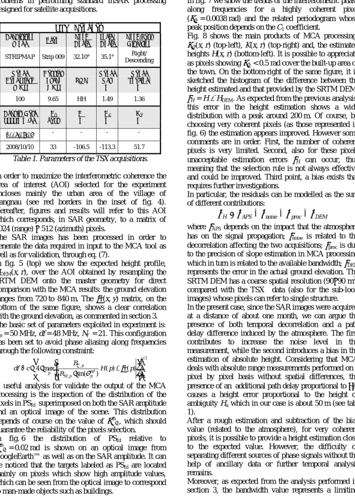
where σ0 is the normalized radar cross section, which we set to 1, A is the area of the metallic planar reflector that we assume to have a squared shape with side of 0.5 m, and Aclutter is the area of the resolution cell which depends on Bp. In fig. 1 we sketch the trend of the propagated errors on the height difference, σ∆R (top) and that on the cycle number, σk (bottom) computed from (3)-(4) as a function of Nf, for B ranging from 100 to 400 MHz and Bp = 40 MHz. Both figures decrease as Nf increases whith a trend saturation which depends on B. The estimation of both ∆R and k are expected to improve as B, and consequently Be, increase. Moreover, in Figs. 2 and 3 we show the trends of the same parameters for different Bp values and for B = 100 MHz and B = 400 MHz, which are the bandwidth values of the real dataset available for the present experiment. As expected, the estimation is improved by using wider Bp and in turn the maximum allowable Bp value increases as B increases.

Of course this estimation is performed in favourable setting, thus results from real data are expected show worst performances.

This analysis points out the importance of bandwidth in MCA. In particular, a value of 100 MHz seems to be inadequate for a reliable application of MCA for absolute difference path retrieval (∆R) as well as for fringe classification though k values estimation, even when using a large number of sub-looks. For instance, the condition for proper k value determination is

σk << 1, which is rarely satisfied by using B = 100 MHz, even in the simulated favourable scenario of a very coherent scatterer. This analysis is confirmed by performing MCA on a real SAR dataset, as shown in the following section.

5. SAR DATASETS

Two SAR datasets were available for the present study: one acquired from airplane, hereafter referenced to as AES-1 dataset, the other acquired from satellite, hereafter indicated as TSX dataset.

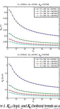
The AES-1 dataset was acquired by bistatic antennas mounted on an airplane and operating at X band with a total radar bandwidth of 4×100 MHz resulting from four non-overlapping channels each 100 MHz wide, whose central frequencies are 9.4, 9.5, 9.6, and 9.7 GHz, respectively. The sampling frequency fs is 200 MHz, corresponding to a slant range spacing of 0.75 m. The synthesized Doppler bandwidth is 50 Hz with a resulting azimuth resolution of 1.5 m. The area covered by the AES-1 dataset (yellow borders in fig. 4) is a scarcely urbanized area located in Switzerland close to the town of Langnau, with an extension of about 2×2.5 km2.

The TSX dataset consists of a pair of InSAR images obtained from the TerraSAR-X archive and acquired on 07/09/2008 and 10/10/2008, respectively, which include the same area around Langnau as the AES-1 dataset (see red borders in fig. 4). Table 1 reports some relevant parameters of the acquisitions. Data are acquired in stripmap mode, along descending orbits, with 100 MHz range bandwidth and ~32 degrees look angle. The September acquisition has been selected as master image for the InSAR processing. In order to minimise both temporal and geometrical decorrelation, the images have been selected by minimising the temporal and spatial distance: Bt = 33 days, B⊥ = −106.5 m.

6. RESULTS FROM TERRASAR-X DATASET

In this section we present the results of a first application of MCA to SAR Level-1 data by using the TSX dataset presented in the previous section.

This choice was driven by the possibility to obtain the data needed for validation by using a standard InSAR pre-processing. Although the airborne AES-1 dataset appears more promising in term of both bandwidth and coherence, it presents some fluctuations related to both geometric and radiometric parameters as well as some

problems in performing standard InSAR processing designed for satellite acquisitions.

TSX (Langnau) Acquisition Mode Beam Look Angle Incid. Angle Look/Pass Direction

STRIPMAP Strip 009 32.10° 35.1° Right/

Descending Range Bandwidth (MHz) Carrier Freq. (GHz) POL Range Res. (m) Range Spacing. (m) 100 9.65 HH 1.49 1.36 Acquis. Date yyyy/mm/dd Bt (days) B┴ (m) B// (m) Ha (m) 2008/09/07 - - - - 2008/10/10 33 -106.5 -113.3 51.7

Table 1. Parameters of the TSX acquisitions. In order to maximize the interferometric coherence the area of interest (AOI) selected for the experiment encloses mainly the urban area of the village of Langnau (see red borders in the inset of fig. 4). Hereafter, figures and results will refer to this AOI which corresponds, in SAR geometry, to a matrix of 1024 (range) × 512 (azimuth) pixels.

The SAR images has been processed in order to generate the data required in input to the MCA tool as well as for validation, through eq. (7).

In fig. 5 (top) we show the expected height profile, HDEM(x, r), over the AOI obtained by resampling the SRTM DEM onto the master geometry for direct comparison with the MCA results: the ground elevation ranges from 720 to 840 m. The δr(x, y) matrix, on the bottom of the same figure, shows a clear correlation with the ground elevation, as commented in section 3. The basic set of parameters exploited in experiment is: Bp = 50 MHz, df = 48 MHz, Nf = 21. This configuration has been set to avoid phase aliasing along frequencies through the following constraint:

1 , , ) ( ) ( ) sin( max 4 − ⊥ ⎥ ⎥ ⎦ ⎤ ⎢ ⎢ ⎣ ⎡ ⎟ ⎟ ⎠ ⎞ ⎜ ⎜ ⎝ ⎛ − ⋅ ⋅ ⋅ < H p r p R B c df p p M p p ϑref δ

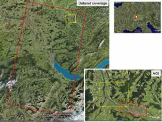
A useful analysis for validate the output of the MCA processing is the inspection of the distribution of the pixels in PSfd superimposed on both the SAR amplitude and an optical image of the scene. This distribution depends of course on the value of σthΦ, which should guarantee the reliability of the pixels selection.

In fig. 6 the distribution of PSfd relative to σth

Φ = 0.02 rad is shown on an optical image from GoogleEarth™ as well as on the SAR amplitude. It can be noticed that the targets labeled as PSfd are located mainly on pixels which show high amplitude values, which can be seen from the optical image to correspond to man-made objects such as buildings.

In fig. 7 we show the trends of the interferometric phase along frequencies for a highly coherent pixel (σΦ = 0.0038 rad) and the related periodogram whose peak position depends on the C1 coefficient.

Fig. 8 shows the main products of MCA processing:

σΦ(x, r) (top-left), K(x, r) (top-right) and, the estimated

heights H(x, r) (bottom-left). It is possible to appreciate as pixels showing σΦ < 0.5 rad cover the built-up area of the town. On the bottom-right of the same figure, it is sketched the histogram of the difference between the height estimated and that provided by the SRTM DEM:

εH = H − HDEM. As expected from the previous analysis, this error in the height estimation shows a wide distribution with a peak around 200 m. Of course, by choosing very coherent pixels (as those represented in fig. 6) the estimation appears improved. However some comments are in order. First, the number of coherent pixels is very limited. Second, also for these pixels unacceptable estimation errors εH can occur, thus meaning that the selection rule is not always effective and could be improved. Third point, a bias exists that requires further investigations.

In particular, the residuals can be modelled as the sum of different contributions: DEM proc noise APS H

ε

ε

ε

ε

ε

=

+

+

+

where εAPS depends on the impact that the atmosphere has on the signal propagation; εnoise is related to the decorrelation affecting the two acquisitions; εproc is due to the precision of slope estimation in MCA processing which in turn is related to the available bandwidth; εDEM represents the error in the actual ground elevation. The SRTM DEM has a coarse spatial resolution (90×90 m2) compared with the TSX data (also for the sub-look images) whose pixels can refer to single structure. In the present case, since the SAR images were acquired at a distance of about one month, we can argue the presence of both temporal decorrelation and a path delay difference induced by the atmosphere. The first contributes to increase the noise level in the measurement, while the second introduces a bias in the estimation of absolute height. Considering that MCA deals with absolute range measurements performed on a pixel by pixel basis without spatial differences, the presence of an additional path delay proportional to λ/2 causes a height error proportional to the height of ambiguity Ha which in our case is about 50 m (see tab. 1).

After a rough estimation and subtraction of the bias value (related to the atmosphere), for very coherent pixels, it is possible to provide a height estimation close to the expected value. However, the difficulty of separating different sources of phase signals without the help of ancillary data or further temporal analysis remains.

Moreover, as expected from the analysis performed in section 3, the bandwidth value represents a limiting

factor in the MCA performace. In the next section we try to evaluate the impact of this parameter on height retrieval through MCA processing.

7. RESULTS FROM AIRBORNE AES-1

DATA-SET

Using the AES-1 dataset provides the possibility to explore different values of bandwidth from 100 to 400 MHz. For this dataset the normal baseline B⊥ is 0.75 m, thus ensuring a very limited geometrical decorrelation effect. Moreover, since the two antennas acquire simultaneously, temporal decorrelation and atmospheric contributions to the interferometric phase are avoided (εAPS = εnoise ≅ 0). This configuration thus appears very promising for MCA testing in particular for what concerns the impact of the bandwidth value on

εH.

However, airborne data present some fluctuations in some geometrical parameters, and in the present case it was not possible to provide univocal values needed to evaluate eq. (7) for direct height comparison and validation. Moreover, inspection of the metadata pointed out the presence of a delay along the hardware acquisition line of one of the two antenna. Since the inspection did not allow to define the actual value of this delay, it resulted impossible to perform absolute interferometric phase estimation. For these reasons, the experiment with AES-1 data was performed by analysing the data in slant range geometry without a direct comparison with the SRTM height profile. Anyway, this limitation did not prevent to verify how the MCA performances depend on the available bandwidth. The area selected for the test is sketched in yellow in the inset figure of fig. 1. Fig. 9 shows the reflectivity map (left) and InSAR phase field (right) for a single sub-look acquisition at 100 MHz. Fig. 10 shows the k values distribution computed through MCA analysis by using different bandwidths (400, 300, 200 and 100 MHz). The k values are related to the interferometric fringes pattern in fig. 9 (right): each fringe corresponds to a certain k value. It can be noted that the k values map obtained by processing a bandwidth of 400 MHz reproduces properly the fringe pattern. To provide a numerical proof, we selected the range line sketched on the interferometric phase fields in fig. 9 and, on the k values map at 400 MHz in fig. 10 (top-left): along this range line, 11 interferometric fringes can be counted, and correspondingly 11 k value classes. It is worthwhile to point out that the k values map is computed on a pixel by pixel basis without any spatial integration of the information. This means that the number of k value classes can be inferred by the difference between the k values computed on two pixels PSfd located at near and far range respectively. This is not true for the InSAR phase which involves spatial differences between neighbouring pixels.

The images in fig. 10 show clearly the performance of the measure as a function of the spanned bandwidth: as the bandwidth becomes narrower, the fringe classification appears noisier. A bandwidth of least 300 MHz seems to be required to provide reliable results. In particular, it results evident that for B = 100 MHz the correlation with the fringe pattern disappears. Therefore, a bandwidth of 100 MHz appears inadequate for reliable height inference. It is worthwhile to remember that the AES-1 dataset it is not affected neither by atmospheric distortion, nor by temporal decorrelation, and also the geometrical decorrelation is extremely limited. Therefore, this experiment confirms that, in the case of TerraSAR-X dataset, where the phase information is corrupted by temporal and geometrical decorrelation and by the presence of atmospheric signal, a bandwidth of 100 MHz leads to unreliable height estimation as reported in the previous section.

The maps in fig. 11 show the k values only for pixels in PSfd. The threshold σthΦ which defines PSfd has different values in order to guarantee the same reliability in k estimation. Indeed, as the bandwidth becomes narrower, the number of samples along frequencies decreases and the fit along frequencies becomes less reliable. The number of pixels in PSfd in the case of B = 100 MHz (map at the bottom-right) results extremely low.

Figure 1. σ∆R (top), and σk (bottom) trends as a function of Nf computed for B ranging from 100 to 400 MHz and

Bp = 40 MHz. 0 10 20 30 40 50 60 0 0.5 1 1.5 2 2.5 N_f σK (2 π uni t) fo = 9.65GHz , Bp = 40 MHz , σ_φ = 0.057548 B = 100 , Be = 60 MHz B = 200 , Be = 160 MHz B = 300 , Be = 260 MHz B = 400 , Be = 360 MHz 0 10 20 30 40 50 60 0 0.005 0.01 0.015 0.02 0.025 0.03 0.035 N_f σR∆ (m ) fo = 9.65GHz , Bp = 40 MHz , σ_φ = 0.057548 B = 100 , Be = 60 MHz B = 200 , Be = 160 MHz B = 300 , Be = 260 MHz B = 400 , Be = 360 MHz

Figure 2. σ∆R trends as function of Nf, for Bp ranging from 20 to 200 MHz and B = 100 MHz (top) and

B = 400 MHz (bottom).

Figure 3. σk trends as a function of Nf, for Bp ranging from 20 to 200 MHz and B = 100 MHz (top) and

B=400 MHz (bottom).

Figure 4Red and yellow borders enclose the areas covered by the AES-1 and TSX SAR data respectively.

The sample areas selected for the processing are sketched in the inset figure.

Figure 5. SRTM heights (top) and δr matrix (bottom) for the TSX AOI in meters.

0 5 10 15 20 25 30 35 40 0 0.002 0.004 0.006 0.008 0.01 0.012 0.014 N_f σR∆ (m ) fo = 9.65GHz , B = 400 Bp = 20 , Be = 200 MHz , σφ = 0.0814 Bp = 80 , Be = 200 MHz , σφ = 0.0407 Bp = 140 , Be = 200 MHz , σφ = 0.0308 Bp = 200 , Be = 200 MHz , σ_φ = 0.0257 0 5 10 15 20 25 30 35 40 0.01 0.02 0.03 0.04 0.05 0.06 0.07 N_f σR∆ (m ) fo = 9.65GHz , B = 100 Bp = 20 , Be = 40 MHz , σ_φ = 0.0814 Bp = 40 , Be = 40 MHz , σφ = 0.0575 Bp = 60 , Be = 40 MHz , σ_φ = 0.047 0 5 10 15 20 25 30 35 40 0.1 0.2 0.3 0.4 0.5 0.6 0.7 0.8 0.9 N_f σK (2 π uni t) fo = 9.65GHz , B = 400 Bp = 20 , Be = 200 MHz , σ_φ = 0.0814 Bp = 80 , Be = 200 MHz , σφ = 0.0407 Bp = 140 , Be = 200 MHz , σ_φ = 0.0308 Bp = 200 , Be = 200 MHz , σφ = 0.0257 0 5 10 15 20 25 30 35 40 0.5 1 1.5 2 2.5 3 3.5 4 4.5 N_f σK (2 π un it ) fo = 9.65GHz , B = 100 Bp = 20 , Be = 40 MHz , σ_φ = 0.0814 Bp = 40 , Be = 40 MHz , σ_φ = 0.0575 Bp = 60 , Be = 40 MHz , σ_φ = 0.047

Figure 6. Distribution of PSfd relative to a σthΦ= 0.02 rad shown on an optical image provided by GoogleEarth™ (top) as well as on the SAR amplitude

(bottom).

Figure 7. Interferometric phase trend and related periodogram of a coherent pixel (σΦ = 0.0038 rad).

Figure 8. Main products of MCA processing: σΦ(x, r) (top-left), K(x, r) (top-right) and, the estimated heights H(x, r) (bottom-left). The histogram of εH = H − HDEM

is also sketched on the bottom-right.

Figure 9. Reflectivity map (left) and InSAR phase field (right) for the AES-1 dataset. The data refer to a single

sub-band acquisition at 100 MHz.

Figure 10. Kvalues maps computed through MCA analysis by using different bandwidth (400, 300, 200

and 100 MHz, respectively).

Figure 11. K values maps on pixels selected according to σthΦ and computed through MCA analysis by using

different bandwidth (400, 300, 200 and 100 MHz respectively).

8. CONCLUSIONS

This paper has introduced the MCA and provided some details relative to its implementation and validation. Through a parametric analysis, the limits of applicability of the technique according to the processing parameter and the available bandwidth have been evaluated. Then, a first validation experiment has been performed by using both Level 1 TerraSAR-X data and AES-1 airborne data.

It has been also demonstrated that, in the case of AES-1 dataset, which is not affected by neither atmospheric distortions nor temporal and geometrical decorrelation, a bandwidth of least 300 MHz seems to be required to provide reliable results. This result confirms the evaluation obtained by the parametric analysis designed under favourable conditions.

In the case of TerraSAR-X dataset, where the phase information is corrupted by temporal and geometrical decorrelation and by the presence of atmospheric signal, a bandwidth of 100 MHz leads to unreliable height estimation. Thus, the application of MCA for height retrieval by using satellite data requires wider bandwidth and needs further investigations.

However, increasing bandwidths is not the only action possible. For example, benefits could derive by integrating an independent method to measure the integral atmospheric delay during the data takes, based on a combination of wide area mapping (possibly supported by an atmospheric model) and calibration coherent scatterers on the test site.

The data analysis pointed out also that the criterion for target selection based on a threshold on σΦ may result occasionally unreliable, thus requiring further developments to increase the robustness of the selection. The technique has shown its potential in measuring ground elevation, when proper bandwidth is available and provided the atmospheric signal can be evaluated and removed. Moreover, the approach can also be used to support standard phase unwrapping as well as to investigate the scattering properties of the targets [7]. Future work will be devoted to process TerraSAR-X spotlight data with a bandwidth of 300 MHz and to add temporal analysis for atmospheric signal filtering.

9. ACKNOWLEDGEMENTS

Work supported by ESA ESTEC Contr. N. 21319/07/NL/HE. Sample AES-1 data courtesy of SARMAP, while TerraSAR-X images are provided by DLR under a Scientific Use License for proposal MTH0397. The authors thank Ing. Davide Nitti from Politecnico di Bari for his help in pre-processing TSX data.

10. REFERENCES

[1] N. Veneziani, F. Bovenga, and A. Refice, “A wide-band approach to absolute phase retrieval in SAR interferometry”. Multidimensional Systems and Signal Processing, vol. 14, no. 1-2, 2003.

[2] F. Bovenga, V. M. Giacovazzo, A. Refice, N. Veneziani, R. Vitulli, “First validation experiment for a multi-chromatic analysis (MCA) of SAR data starting from SLC images”, Proc. IGARSS 2009, Cape Town, South Africa, July 13-17, 2009.

[3] T. Toutin, L. Gray, “State-of-the-art of elevation extraction from satellite SAR data”, ISPRS Journal of Photogrammetry & Remote Sensing, vol. 55, pp. 13–33, 2000.

[4] Hanssen, R. F., Radar Interferometry: Data Interpretation and Error Analysis, Kluwer Academic Publishers, Dordrecht (2001).

[5] G. Ketelaar, P. Marinkovic, and R. Hanssen, “Validation of point scatterer phase statistics in multi-pass InSAR,” in Proc. CEOS SAR Workshop, Ulm, Germany, May 27–28, 2004.

[6] A. Ferretti, G. Savio, R. Barzaghi, A. Borghi, S. Musazzi, F. Novali, C. Prati, and Fabio Rocca, “Submillimeter Accuracy of InSAR Time Series: Experimental Validation”, IEEE TGRS, vol. 45, n. 5, May 2007.

[7] Giacovazzo, A. Refice, F. Bovenga, N. Veneziani, “Identification of coherent scatterers: spectral correlation vs. Multi-Chromatic Phase Analysis ”, in Proc. of IGARSS 2008, Boston, Massachusetts, USA, July 6-11, 2008.