PIRLS: Poisson Iteratively Reweighted Least Squares Computer Program for Additive, Multiplicative, Power, and Non-linear Models

(1)

PIRLS: Poisson Iteratively Reweighted Least Squares Computer

Program for Additive, Multiplicative, Power, and Non-linear Models

Leif E. Peterson

Center for Cancer Control Research

Baylor College of Medicine

Houston, Texas 77030

November 3, 1997

Abstract

A computer program to estimate Poisson regression coefficients, standard errors, Pearsonχ2 and deviance goodness of fit (and residuals), leverages, and Freeman-Tukey, standardized, and deletion residuals for additive, multiplicative, power, and non-linear models is described. Data used by the program must be stored and input from a disk file. The output file contains an optional list of the input data, observed and fitted count data (deaths or cases), coefficients, standard errors, relative risks and 95% confidence intervals, variance-covariance matrix, correlation matrix, goodness of fit statistics, and residuals for regression diagnostics.

Key Words: Poisson Regression, Iteratively Reweighted Least Squares, Regression Diagnostics, Matrix Ma-nipulation.

1 INTRODUCTION

1.1 Poisson Distribution

Poisson regression models are commonly used for modeling risk factors and other covariates when the rates of disease are small, i.e., cancer [1, 2, 3, 4, 5]. An area of research in which Poisson regression of cancer rates is commonly employed is the investigation of radiation-induced cancer among Hiroshima and Nagasaki atomic bomb survivors [6, 7, 8] and individuals occupationally [9], medically [10] and environmentally [11] exposed to ionizing radiation. Poisson regression has also been used to investigate the effects of information bias on lifetime risks [12], diagnostic misclassification [13, 14], and dose-response curves for radiation-induced chromosome aberrations [15]. Several computer programs have been developed that perform Poisson regression [16, 17, 18, 19, 20]. While the PREG program [3] can fit additive, multiplicative, and non-linear models, it does not provide the capability to fit power models nor perform regression diagnostics. This report documents the PIRLS Poisson regression algorithm for fitting additive, multiplicative, power, and non-linear models and regression diagnostics using leverages of the Hat matrix, deletion and standardized residuals.

The critical data required to apply the computer code are:

• Number of cases for each stratum

• Number of person-years for each stratum

• Design matrix of independent variables

There is only one output format, listing the input data, observed and fitted count data (deaths or cases), coeffi-cients, standard errors, relative risks (RR) and 95% confidence intervals, variance-covariance matrix, correlation matrix, goodness of fit statistics, and residuals for regression diagnostics. The program and all of its subroutines

(2)

are written in FORTRAN-77 and are run on a desktop PC with a AMD-K6-166MHz(MMX) chip. The algorithm can be compiled and run on Unix machines as well. The PC version of the executable requires 180,224 bytes of random access memory (RAM) to operate. Average execution time is several seconds per run, depending on the amount of input data.

2 PROGRAM DESCRIPTION

The computer program proceeds as follows. During run-time, the user interface with the program involves the following:

• Specifying the type of model to be fit (1-additive, 2-multiplicative, 3-power, and 4-non-linear)

• For additive models, specifying the power,ρ, which ranges from 1 for purely additive models to 0 for purely multiplicative models

• Specifying the number of independent variables (not cases or person-years) that are to be read from the input file

• Specifying the number of parameters to estimate

• For non-linear models, optional starting values for parameters

• For multiplicative models, specifying if the regression coefficients are to be exponentiated to obtain RR and its 95% CI

• Specifying whether or not the variance-covariance and correlation matrices are written to the output file whose name is specified by the user

• Specifying whether or not the input data are written to the output file whose name is specified by the user

• Specifying whether or not the observed and fitted count data (deaths or cases) are written to the output file

• Specifying whether or not the leverages, and standardized and deletion residuals are written to the output file

Once the data above have been specified during run time, the program does the following:

1. First, a “starting” regression is performed by regressing the ratio of counts (deaths or cases) to person-years of follow-up as the dependent variable on the independent variables. For non-linear models, the default starting regression can be skipped by specifying starting values for each parameter.

2. The difference between the observed and fitted counts (error residuals) from the starting regression are used as the dependent variable and regressed on the cross product of the inverse of the information matrix (variance covariance-matrix) and the score vector to obtain the solution vector.

3. The solution vector is then added to the original regression coefficients obtained during the starting regres-sion.

4. Iterations are performed until the sum of the solution vector is below a fixed value called theconvergence criterion, for which the default in PIRLS is 10−5.

5. After convergence is reached, the standard errors are obtained from the diagonal of the variance-covariance matrix, and if specified, residuals for regression diagnostics are estimated.

6. Depending on specifications made by the user, various data are written to the output file, and then the program terminates run-time.

3 NOTATION AND THEORY

3.1 Binomial Basis of Poisson Regression

For largenand smallp, e.g., a cancer rate of say 50/100,000 population, binomial probabilities are approximated by the Poisson distribution given by the form

P(x) = e

−m

(3)

Table 1: Deaths from coronary disease among British male doctors [21]. Non-smokers Smokers Age group,i di Ti λi(0) di Ti λi(1) 35-44 2 18,790 0.1064 32 52,407 0.6106 45-54 12 10,673 1.1243 104 43,248 2.4047 55-64 28 5,710 4.9037 206 28,612 7.1998 65-74 28 2,585 10.8317 186 12,663 14.6885 75-84 31 1,462 21.2038 102 5,317 19.1838

where the irrational numbere is 2.71828.... In many respects, the Poisson distribution has been widely used in science and does not really have a direct relationship with the binomial distribution. As such,npis replaced by µin the relationship

f(x) =µ x_e−µ

x! , (2)

whereµis the mean of the Poisson distribution. It has been said that as long asnpqis less than 5, then the data are said to be Poisson distributed.

3.2 Poisson Assumption

The Poisson assumption states that, for stratified data, the number of deaths, d, in each cell approximates the valuesx=0,1,2,... according to the formula

P(d=x) = (λT)e

−λT

x! , (3)

whereλis the rate parameter which is equal to the number of deaths in each cell divided by the respective number ofperson-years (T) in that same cell. As an example, Table 1 lists a multiway contingency table for the British doctor data for coronary disease and smoking [21]. The rates for non-smokers, λi(0), are simply the ratio of the number of deaths toTi in age groupiand exposure group 0, whereas the rates for smokers, λi(1), are the ratio of deaths toTiin age groupifor the exposure group 1.

3.3 Ordinary Least Squares

Let us now look into the sum of squares for common linear regression models. We recall that most of our linear regression experience is with the model

Y=Xβ+ε, (4)

whereYis a column vector of responses,Xis the data matrix,βis the column vector of coefficients andεis the error. Another way of expressing the observed dependent variable,yi, of (4) inmodel terms is

yi=β0+β1xi1+β2xi2· · ·βjxij+εi, (5)

and in terms of thepredicted values, ˆyi, is ˆ

yi= ˆβ0+ ˆβ1xi1+ ˆβ2xi2· · ·βjxijˆ +ei. (6)

The residual sum of squares of (6) is

SS(β) = Pn_i₌₁{yi−yˆi}2 = Pn_i₌₁e2_i = e0e.

(4)

Because of the relationship

e=Y−Xβ, (8)

we can rewrite (7) in matrix notation as

SS(β) = (Y−Xβ)0(Y−Xβ). (9)

3.4 Partitioning Error Sum of Squares for Weighted Least Squares

Suppose we have the general least squares equation

Y=Xβ+ε. (10)

and according to Draper and Smith [22] set

E(ε) =0 V(ε) =Vσ2 ε∼N(0,Vσ2), (11) and say that

P0P=PP=P2=PP=V. (12)

Now if we let

f=P−1ε E(f) =0, (13)

and then premultiply (10) byP1, as in

P−1Y=P−1Xβ+P−1ε, (14)

or

Z=Qβ+f. (15)

By applying basic least squares methods to (14) the residual sums of squares is

f0f=ε0(P−1)0P−1ε, (16) since (P−1ε)0=ε0(P−1)0, (17) and since (B−1A−1) = (AB)−1, (18) then f0f =ε0(PP)−1ε, (19) which is equivalent to f0f =ε0(V)−1ε. (20)

The sum of squares residual then becomes for (14)

SS(β) = (Y−Xβ)0V(Y−Xβ). (21)

3.5 Partitioning Error Sum of Squares for Iteratively Reweighted Least Squares

According to McCullagh and Nelder [23], ageneralized linear model is composed of the following three parts:

• Randomcomponent,λ, which is normally distributed with mean _T1

i ·µiand variance

µi

T_i2.

• Systematiccomponent,x, which are covariates related to the linear predictor, (x0_iβ), by the form (x0_iβ) =

p

X

j=1

(5)

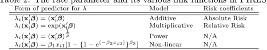
Table 2: The rate parameter and its various link functions in PIRLS.

Form of predictor forλ Model Risk coefficients

λi(x0_iβ) = (x0_iβ) Additive Absolute Risk

λi(_x0_i_β) = exp(_x0_i_β) Multiplicative Relative Risk

λi(x0_iβ) = (x0_iβ)1ρ Power N/A

λi(x0_iβ) =β₁x_i₁[1− {1−e(−β2xi2)_}β3] Non-linear N/A

• Thelinkbetween the random and systematic components for a linear model is given by

λi=λi(xi0β), (23)

where λi is theobserved rate parameter and λi = (xi0β) is thepredicted rate parameter. It should be pointed out that the rate parameter, λi = (xi0β), serves as its own link function. Thus, the rate parameter provides a linearization of our distributional models so that we can use multiple linear regression to obtain Best Linear Unbiased Estimators (BLUEs). In effect, the rate parameter allows us to reduce non-linear (non-Gaussian) models to linear models so that we can solve the system of linear equations. The rate parameter can take on various linear and non-linear functions. These are shown in Table 2. The power transformation was adapted from [24].

As shown in Table 2, it is obvious that the random component,λi, can take on a non-linear relationship with the systematic component,x. Tolinearizeλi in a least squares approach by a succession of stages oriterations, we carry out a Taylor series expansion ofλiabout a pointβ0. Since we know that

g(β) =g(β0) +g(β0)0(β−β0), (24) a Taylor series expansion ofλiabout (β−β0) gives us

λi'λi(x0_iβ0) + p X j=1 h_∂λ i(x0_iβ) ∂βj i β=β₀(β−β0) +ei. (25) Rearranging this equation, we have

λi−λi(x0_iβ0) =Z0δ0+ei, (26) where Z0_ij= h_∂λ i(x0β) ∂β_j i β =β0 , (27) and δ_i0=βi−βi0. (28)

TheJacobianmatrix of partial derivatives ofλi(x0_iβ) with respect to the parameters,βat the zeroth iteration is then Z₀=     z11 z12 · · · z1p z21 z22 · · · z2p . .. ... . .. ... zn1 zn2 · · · znp    =Z0_ij,n×p. (29)

From (26), the residuals,ei, now become

(6)

3.5.1 Development of Dependent Variable, Y

Using (30), letλi−λ0i(x0iβ) be equal toYi. We now rewrite the residuals

ei=Yi−Zδ, (31)

so that the column vector,Yof dependentYbecomes

Y=     λ1−λ0₁(x0₁β) λ2−λ0₂(x0₂β) . .. λn−λ0n(x0nβ)    . (32)

3.5.2 Development of Weighting Matrix, W

We know thatV ar(cX) =c2V ar(X) so if we substitute in ˆλwe have

V ar(_T1 i ·µi)ˆ = 1 Ti 2 V ar( ˆµi) = µˆi T_i2. (33)

Therefore, each diagonal element of theweightmatrix becomes wii= 1 V ar( ˆλi) = T_i2 ˆ µi =Ti·Ti ˆ λi·Ti = Ti ˆ λi. (34)

Becauseλi can be very small andTivery large and it is better to divide by a larger number than a smaller one with a computer, we will we choose the weight Ti2

µi. The entire weighting matrixW is then

W=       T₁2 ˆ µ1 0 0 0 0 T_µ_ˆ22 2 0 0 .. . ... . .. ... 0 0 · · · Tn2 ˆ µn      . (35)

3.5.3 Defining Maximum Likelihood Solution Vector, δ

Let V−1 =W, and now substitute our new definition for residuals from (31) into (21) obtain the new sum of squares

SS(δ) = (Y−Zδ)0W(Y−Zδ) (36)

= WY0Y−(Zδ)0WY−Y0ZWδ+δ0Z0WZδ. (37) The transpose (Zδ)0 of the term (Zδ)0WY in (37) is equal toδ0Z0 because (AB0 =B0A0). In addition, since (Zδ)0WYis a 1×1 matrix, or scalar, then its transposeY0ZWδ0has the same value. Thus, (37) is transformed into

SS(δ) =WY0Y−2δ0Z0WY+δ0Z0WZδ. (38) Theδ0on the left sides of parameters in the right side of (38) drop out because if we set

A= (Z0WY), (39)

and from Searle [25] know that

∂x0A

(7)

and if we set

A= (Z0WZδ), (41)

and from [25] know that

∂(x0Ax)

∂x = 2Ax, (42)

then the normal equation then becomes

SS(δ) =Z0WZδ+Z0WY. (43)

In order to minimize (43) with respect to theδ parameters, we must take the first partial derivative. This gives us

∂SS(δ) ∂δ =−2Z

0_WY_{+ 2(}_Z0_WZ_δ₎_, ₍₄₄₎

that provides us with the consistent equations

(Z0WZδ) =Z0WY, (45)

that has solution

δ= (Z0WZ)−1Z0WY. (46) At theith iteration, the values of the parameters are

βi=βi−1+δ. (47) Convergence is reached at the point when

{βi−β(i−1)}/β(i−1)< , (48) whereis 10−5 by default in PIRLS.

3.6 Variance-covariance Matrix

The variance-covariance matrix, with parameter variance on the diagonal and covariances on the off-diagonals, at convergence is identical to the information matrix or inverse of the weighted dispersion matrix

I−_β1= (Z0WZ)−1=     σ₁2 σ12 · · · σ1j σ₁₂ σ₂2 · · · σ₂j .. . ... . .. ... σ1j σ2k · · · σj2    . (49)

3.7 Standard Errors of Regression Coefficients

The standard errors of the regression coefficients are equivalent topσ_j2. A Wald test for each parameter is simply βj/s.e.(βj) and indicates significance if the ratio is<−1.96 or>1.96 at theα= 0.05 level of significance.

3.8 Residuals and Regression Diagnostics

The error residual,eihas mean 0 and measures the lack of concordance of the observedµiagainst the fitted value ˆ

µi. The greater the value ofei, the worse the fit of the model. Pearson residuals,rP are estimate as rP =

µi−µiˆ

µ , (50)

and provide a measure of the residual variation. The deviance residuals rD=µi h logµi ˆ µi i + ( ˆµi−µi), (51)

(8)

allow the investigator to determine the goodness of fit of the model, i.e., how well the observed data agree with the fitted values. Freeman and Tukey [26] introduced a variance stabilized residual for Poisson models given by

rF T =√µ+

p

µ+ 1−pµˆ+ 1. (52)

The leverage [23] for each observation, hi, provides information about the geometric distance between a given point (zi1, zi2,· · ·, zij) and the centroid of all points (¯zi1,zi¯2,· · ·,zij) in the predictor space. Individual leverages,¯ hi, are obtained from the diagonal of the “Hat” matrix given by

H=√WZ(Z0WZ)−1Z0√W. (53)

Because Phi = trace(H) =p, observations with high leverage can approach unity. A criterion introduced by Hoaglin and Welsch [27] for determing high leverage for an observation states that a point has high leverage if hi >2p/n. Points with high leverage are located at a substantial distance from the fitted regression line, and act to “pull” the fitted line toward their location. Increases in the goodness of fit of a model can be obtained by refitting a model after the observation(s) with high leverage have been removed.

Cook [28] introduced the residual, ∆(β)−ij, which measures the difference betweenβwhen the observation is included in the model andβwhen the observation is not in the model. The more positive the values of ∆(β)−ij, the more influence an observation has when compared with other observations. Individual ∆(β)−ij residuals are obtained by then×pmatrix ∆(β)−ij, by the relationship

∆(β)−ij= −

(Z0WZ)−1zijeijwij

1−hij . (54)

Finally, thestandardized residual is used to measure the model error introduced by particular observation when its error residual has constant variance

˜ ri= ei p (1−hi) . (55)

Values for ˜ri that exceed 1.96 tend to be outliers at theα= 0.05 level of significance.

3.9 Goodness-of-Fit Statistics

The Pearsonχ2 goodness of fit is

χ2= n

X

i=1

rP2, (56)

and the deviance goodness of fit is

D= n

X

i=1

rD, (57)

which is alsoχ2 distributed. If a model fits, itsχ2 andDwill be lower than the degrees of freedom (n−p).

3.10 Structure

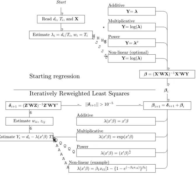
Program flow is outline in Figure 1. The starting regression to obtain the initial values of the parameter vector,

βiis performed by calling:

CALL INIT(NREG, NCOL, NROW, ISTART, START, B, G, RHO, IPRED, IDATA, INFILE, OUTFILE,IFLT) For non-linear models, the user can specifiy starting values for the parameters and skip the multiplicative fit to obtain starting parameter estimates. The solution vector,δ, used to modify the original regression coefficients during each iteration are determined through calls of:

CALL PRED(NCOL, NROW, G, IDF, DEV, TPR, NREG, RHO, IPRED, ZTWZ1, ZTWY, ITER, WIN, YDIFF, OEXPE, OOBS, OFT, OPR, XIN,XT,IFLT)

Lastly, the leverages, deletion residuals, and standardized residuals are obtained by calling: CALL FIT(WIN, YDIFF, XIN, XT, ZTWZ1, OEXPE, LEV, DRES, SRES, NCOL, NROW,IFLT)

(9)

Start ? Readdi,Ti, andX ? Estimateλi=di/Ti, wi=Ti * H H HHj J J J J J J ^ Y=λ Y= log(λ) Y=λρ Y= log(λ) Additive Multiplicative Power Non-linear (optional) ? β= (X0WX)−1X0WY

Starting regression

Iteratively Reweighted Least Squares

βi

? ? β_i+1=δi+1+β_i λ(x0β) =x0β λ(x0β) = exp(x0β) λ(x0β) = (x0β)1ρ λ(x0β) =β1xi1[1− {1−e(−β2xi2)}β3] Additive Multiplicative Power Non-linear (example) + Q Q Q Q Q Q k A A A A A A A A K EstimateYi=di−λ(x0β)Ti 6 Estimatewii,zij 6 δi+1= (Z0WZ)−1Z0WY0 - ||δi+1||>10 −5 -Stop when ||δi+1||<10−5

(10)

The parameter, arrays, and variables used in PIRLS are defined below. MP=4000 Parameter Constant Fixed array size for maximum

num-ber of records

NP=28 Parameter Constant Fixed array size for maximum num-ber of variables

IP=1 Parameter Constant Fixed array size for when 1 is needed NIP=16 Parameter Constant Fixed array when more than 1 is

needed

INFILE Character Input Input filename and path OUTFILE Character Input Output filename and path NROW Integer Input Number of input records read NCOL Integer Input Number of parameters specified by

user

ISTART Integer Input For non-linear models; 0=user spec-ified starting values, 1=starting val-ues estimated by multiplicative fit in subroutine INIT

START Real Input For non-linear models; starting val-ues specified by user when IS-TART=0

IPRED Integer Input Number of parameters to be read in from input file

NREG Integer Input Type of regression model to be fit (1-additive, 2-multiplicative, 3-power, 4-non-linear)

IDATA Integer Input Write input data to output file, 1=yes, 0=no

ICOVAR Integer Input Write variance-covariance and cor-relation matrices to output file, 1=yes, 0=no

ICELLS Integer Input Write observed and fitted counts,di, to output file, 1=yes, 0=no IEX Integer Input Exponentiate regression coefficients

for multiplicative models only, i.e., NREG=2

IREG Integer Input Estimate standardized and dele-tion residuials and leverages, 1=yes, 0=no

RHO Real Input Power transform for power models, ρ

OBS(MP) Real Input Number of deaths or cases in sub-group (record),µi

(11)

T(MP) Real Input Number of person-years of follow-up in subgroup (record), T

X(MP,NP) Real Work Design matrix of input independent variables, X

LAMBDA(MP) Real Work Observed rate,λi LAMHAT(MP) Real Work Predicted rate, ˆλi

EXPE(MP) Real Work Expected deaths or cases in sub-group, ˆµi= ˆλi×T

Y(MP) Real Work Error Residual,Yi=µi−dˆi

W(MP) Real Work Variance weights =

W=T2/Var(ˆλi))

Z(MP,NP) Real Work Jacobian matrix of first partial derivatives,Z

ZTWZ(MP,NP) Real Work Information matrix, (Z0WZ) ZTWZ1(NP,NP) Real Work Inverse of information matrix,

(Z0WZ)−1

ZTWY(NP,1) Real Work Score vector,Z0WY

FT(MP) Real Work Freeman-Tukey residuals,rF T PR(MP) Real Work Pearsonχ2 residuals,rP DEV Real Work Deviance residuals, rD

VARCOV(NP,NP) Real Work Variance-covariance matrix used for output, (Z0WZ)

G(NP,1) Real Work Solution vectors,δ

B(NP,1) Real Work Regression coefficients updated at each iteration, β_i

SE(NP) Real Work Standard error ofβi

CORR(NP,NP) Real Work Correlation matrix of coefficients LL(NP) Real Work Lower bound of 95% confidence

limit for relative risk (multiplicative model only)

UL(NP) Real Work Upper bound of 95% confidence limit for relative risk (multiplicative model only)

ML(NP) Real Work Relative risk (multiplicative model only)

LEV(MP,MP) Real Work Leverages from the Hat matrix,hi DRES(MP,NP) Real Work Deletion residuals, ∆(β)i,j SRES(MP) Real Work Standardized residuals, ˜ri

IDF Integer Work Degrees of freedom used for good-ness of fit

DEV Real Work Deviance goodness of fit,D2_d.f. TPR Real Work Pearsonχ2 goodness of fitχ2_d.f. IFLT Integer Output Premature exit codes

0=Convergence reached 1=NCOL<1

2=NROW<1

3=Degrees of freedom, (NROW-NCOL),<1

4=|Pβj|= 0 5=|PGj|= 0 6=Iterations>100

(12)

3.11 Auxiliary Algorithms

MATMUL[29] performs matrix multiplication for the matrix manipulation.TRNPOStranposes arrays as needed for matrix mulitplication. MATINVcallsSVDCMPbased on [30] to invert the information matrix using singular value decompostion. ALGandGAMAINare used for estimating tabled values ofχ2.

3.12 Restriction

All input parameters are checked for nullity and a fault message is returned if there is an illegal entry.

3.13 Time

A thorough investigation of absolute timing has not been performed; however, it should be noted that execution time is a function of the number of model parameters and effects to be considered.

3.14 Precision

The algorithm may be converted to double precision by making the following changes: 1. ChangeREALtoDOUBLE PRECISIONin the algorithm.

2. Change the constants to double precision.

3. ChangeEXPtoDEXPandALOGtoDLOGin all applicable routines.

4. Make appropriate changes in auxiliary routinesMATMUL, TRNPOS, MATINV, SVDCMP, and in functions ALGandGAMAIN.

3.15 Application - Fitting a Multiplicative Model

3.15.1 Data Arrangement and Partial Derivatives

We shall enumerate the steps required for fitting a multiplicative model. Before we start the regression run, however, we must set up the data file and also determine the first partial derivatives of the rate ratio λwith respect to each parameter in the model.

1. Arranging the data in an ASCII text file. The first step is to arrange our data in an ASCII text file. The typical ASCII text file arrangement of data for a Poisson regression run using data in Table 1 is shown in the following:

Cases T/1,000 Age Smoke

---2. 18.790 1 0 0 0 0 0 12. 10.673 0 1 0 0 0 0 28. 5.710 0 0 1 0 0 0 28. 2.585 0 0 0 1 0 0 31. 1.462 0 0 0 0 1 0 32. 52.407 1 0 0 0 0 1 104. 43.248 0 1 0 0 0 1 206. 28.612 0 0 1 0 0 1 186. 12.663 0 0 0 1 0 1 102. 5.317 0 0 0 0 1 1

where the person-years in Table 1 are divided by 1,000 and the covariates denoting the age group are dummy coded (0,1) with a 1 to indicate that the rates are from a given cell, and whether or not the subgroup smoked.

(13)

2. Determining Partial Derivatives of_λ_i(x0iβ) With Respect to Each _β_j. Next we must write out the partial derivatives of the rate parameter with respect to each parameter (these will be used later in the algorithm). The partial derivatives are used in the JacobianZmatrix to form the scores during each iteration. Thus, each partial derivative forms an element,zij, in the JacobianZmatrix. Given that the partial derivative of an exponentiated functionuin the formeu iseudu, the partial derivative ofλi(x0iβ) with respect to each parameter,βj is as follows:

zij =∂λi(x

0

iβ)

∂βj xij, (58)

3.15.2 Steps in the Algorithm

The following section discusses the steps taken by the algorithm for performing iteratively reweighted least squares. 1. Definition of the model. The model we will fit is a log-linear model

λi(x0iβ) =e(β1xi1+β2xi2+β3xi3+β4xi4+β5xi5+β6xi6), (59)

which is equivalent to

log(λi(x0_iβ)) = (β1xi1+β2xi2+β3xi3+β4xi4+β5xi5+β6xi6). (60) 2. Estimate column vector of dependent variables for the log-linear model. The algorithm starts by reading in the data from the input file and then estimates the rate parameter,λi, for each record as the ratio of number ofobserveddeaths to the number ofobservedperson-years. The log ofλiis then calculated to obtain the dependent variable column vector

Y=                  log( d1 T /1,000) log( d2 T /1,000) log( d3 T /1,000) log( d4 T /1,000) log( d5 T /1,000) log( d6 T /1,000) log( d7 T /1,000) log( d8 T /1,000) log( d9 T /1,000) log( d10 T /1,000)                  . (61)

and when substituting in the data above we get

Y=               log(₁₈_.2₇₉₀) log(₁₀12_.₆₇₃) log(₅_.28₇₁₀) log(₂_.28₅₈₅) log(₁_.31₄₆₂) log(₅₂32_.₄₀₇) log(₄₃104_.₂₄₈) log(₂₈206_.₆₁₂) log(₁₂186_.₆₆₃) log(₅102_.₃₁₇)               . (62)

(14)

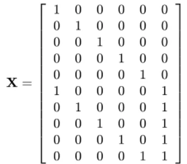
3. Construction of the X matrix of independent variables. In addition to the estimation of the depen-dent variable Ycolumn vector, the algorithm constructs theX matrix of independent variables from the independent variables read in from the input file as

X=               1 0 0 0 0 0 0 1 0 0 0 0 0 0 1 0 0 0 0 0 0 1 0 0 0 0 0 0 1 0 1 0 0 0 0 1 0 1 0 0 0 1 0 0 1 0 0 1 0 0 0 1 0 1 0 0 0 0 1 1               . (63)

4. “Starting Regression” - log-linear regression to estimate initial values of parameters. Once the YandXmatrices are constructed, the algorithm fits the log-linear model

log(λi(x0iβ)) = (β1x1+β2x2+β3x3+β4x4+β5x5+β6x6), (64) which in matrix terms is given as

β= (X0WX)−1X0WY, (65) where diagonal elements ofWare set equal toT. Figure 1 shows the program flow in PIRLS for the various models. Table 3 shows the link functions forλfor each starting regression and the linear predictor used for estimatingλi(x0iβ) during subsequent iterations.

Table 3: Link functions used during “starting regression” and linear predictor used to estimate ˆλduring subsequent iterations.

Model Link function forλ Form of predictor forλ_i(x0_iβ)

Additive _λ_i _λ_i(_x0_i_β) = (_x0_i_β)

Multiplicative log(λ_i) λ_i(x0_iβ) = exp(x0_iβ)

Power λρ_i λi(x_i0β) = (x0_iβ)1ρ

Non-linear (optional)∗ log(λ_i) λ_i(x0_iβ) = exp(x0_iβ)

∗_{For non-linear models, the user can specifiy starting values for}

parameters, rather than using the default multiplicative fit to obtain starting values.

5. Estimation of predicted rate parameter. After the first regression oriteration, the regression coeffi-cients,βj, are used to estimate predicted rates from the linear predictor

λi(x0_iβ) =e

Pp

j=1xijβj ₌_e(x0iβ)_. ₍₆₆₎

6. Estimation of expected number of deaths. The predicted rates are then multiplied by the observed person-years in each record to give the expected number of deaths as

ˆ

µi=di(x0iβ) =λi(x0iβ)Ti. (67) 7. Estimation of dependent variable. The expected number of deaths, ˆµ, are then subtracted from the

observed deaths, ˆµ, to give the dependent variable

Yi=µi−µiˆ =di−λi(x0_iβ)Ti. (68) 8. Construction of column vector Y.The column vectorYis then equal to [Yi].

(15)

Table 4: Survival data for splenic stem cell colony formation after irradiation and transplantation (see ref. [31]). Colonies,µ Trials, Ti Cell concentration,xi1 Dose(Sv),x_i2

60.0 6.0 1.25 0.00 66.0 7.0 1.75 0.96 46.0 4.0 3.00 1.92 82.0 9.0 7.20 2.88 105.0 11.0 24.00 4.32 123.0 15.0 75.00 5.76 12.0 4.0 120.00 6.72

9. Estimation of the partial derivatives for each row vector of the data matrix X. For each record in the data matrix,X, estimate the value of the partial derivatives using the current parameter values,βj. For our log-linear model in (65), we get

zij=∂λi(x 0 iβ) ∂βj =e (x0 iβ)_xij_. ₍₆₉₎

10. Construction of the Jacobian matrix of partial derivatives. Now the algorithm constructs then×p Jacobian matrixZcomposed of the first partial derivatives estimated above, which appears asZ= [zij]. 11. Construction of the inverse variance weighting matrix. Since the Poisson variance of ˆµi changes at

each iteration, we must weight the dispersion matrix with weights defined byT_i2/µˆigiven asW=diag[wii], wherewiiis T

2

i

ˆ

µi.

12. Estimation the solution vector at each iteration. The maximum likelihood solutions at the next and subsequent iterations are obtained through the matrix manipulation

δ= (Z0WZ)−1Z0WY. (70) 13. Updating regression coefficients. At each iteration, the new solution vectors are added to the previous

parameter estimates given as

βi=βi−1+δ. (71) 14. Repeat steps 5-13 above until convergence is reached. The above steps (5 through 13) are repeated

until the euclidean norm of the score vector is below some non-negative value

{βi−β(i−1)}/β(i−1)< , (72) whereis 10−5 by default in PIRLS. At this point, convergence is reached at a global maximum.

3.16 Application - Fitting a Non-linear Model

For this example, we will fit a non-linear model to estimate the number of stem cell colonies in spleens of laboratory mice into which irradiated cells were transplanted [31]. Table 4 shows the colonies formed,µ, number of trials, Ti, cell concentration,xi1, and radiation dose (Sv),xi2, arranged in tabular notation.

The non-linear model we will fit to obtain maximum likelihood estimates of colonies formed is of the form λi=β1xi1[1− {1−e(−β2xi2)_}β3_]_, ₍₇₃₎

where xi1 is the concentration of transplanted cells, xi2 is the radiation dose (Sv), and β1, β2, andβ3 are the parameters of interest.

(16)

In order to build the Jacobian matrix,Z, we need to take the first partial derivatives ofλi with respect toβ1, β₂, andβ₃, i.e.,∂λi/∂β1,∂λi/∂β2, and∂λi/∂β3. Since there are threeβ coefficients, the first column entries for

rowiofZ, i.e.,zi1, will be estimated by use of equation ∂λi

∂β1 =xi1[1− {1−e

(−β2xi2)_}β3_]. ₍₇₄₎

The first partial derivative in the 2nd column entry of rowiofZ, i.e.,zi2 is estimated as ∂λi ∂β2 =−β1xi1{1−e (−β2xi2)_}β3_β 3xi2 e −β2xi2 (1−e−β2xi2). (75) The third column ofZhas elementszi3, which are numerically estimated as

∂λi

∂β₃ =−β1xi1{1−e

(−β2xi2)_}β3_ln(1₋_e−β2xi2₎_. ₍₇₆₎

When fitting this model, we chose to specify starting values ofβ1 = 7.6364, β2 = 0.9341, andβ3 = 7.6364 from [3], rather than use the default multiplicative fit to obtain starting values. Input and output for this model using the data in Table 4 are shown in the Appendix.

3.17 Input

During run-time, the user must respond to the following queries concerning each run:

• The type of model to be fit (1-additive, 2-multiplicative, 3-power, and 4-non-linear)

• For additive models, the power,ρ, which ranges from 1 for purely additive models to 0 for purely multiplica-tive models

• The number of independent (input) variables to be read in from the input file

• The number of parameters to estimate

• For non-linear models, optional starting values for parameters

• For multiplicative models, the regression coefficients are to be exponentiated to obtain RR and its 95% CI

• Whether or not the variance-covariance and correlation matrices are written to the output file

• Whether or not the input data are written to the output file

• Whether or not the observed and fitted count data (deaths or cases) are written to the output file

• Whether or not the leverages, and standardized and deletion residuals are written to the output file

4 USER INPUT DATA FILE

PIRLS uses one input data file (ASCII) whose name is specified by the user at run-time. The input file contains three types of information

1. Run title (text) in record 1

2. FORTRAN format statement (in parentheses) in record 2 needed for reading the input data in later records 3. Input data, i.e., cases, person-years, and independent variables in all subsequent records

The examples in the Appendix give listings of input files.

5 SAMPLE INPUT/OUPUT CASES

The output for all runs is in tabular form in the ASCII text file whose name is specified by the user at run-time. Four examples using an input file are given in the Appendix.

(17)

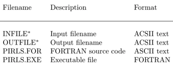
Table 5: Names and descriptions of each PIRLS file.

Filename Description Format

INFILE∗ Input filename ACSII text

OUTFILE∗ Output filename ACSII text

PIRLS.FOR FORTRAN source code ASCII text

PIRLS.EXE Executable file FORTRAN

∗ _{Input and output filenames are specified by user at run-time.}

6 FILENAMES

Table 5 list the names of the files that were used to program, link and execute PIRLS. As one notices, the source code is an ASCII text file and the object and executable files have been compiled with Microsoft FORTRAN Powerstation 4.0. There is one required input data file, whose name is specified at run-time.

7 AVAILABILITY

The program and all of its subroutines are available from the Journal of Statistical Software free of charge at http://www.stat.ucla.edu/journals/jss/

8 ACKNOWLEDGEMENTS

The author is grateful to the reviewers for helpful comments. Work on this algorithm was performed under NASA contract NAS-9 18236.

References

[1] Frome, E.L., Kutner, M.H., Beauchamp, J.J. (1973) Regression analysis of Poisson-distributed data. JASA. 68:935-940.

[2] Frome, E.L. (1983) The analysis of rates using Poisson regression methods. Biometrics. 39:665-674.

[3] Frome, E.L. PREG: A computer program for Poisson regression analysis. Oak Ridge Associated Universities Report ORAU-178 (1981). Oak Ridge National Laboratory. Oak Ridge(TN), ORAU.

[4] Muirhead, C.R., Darby, S.C. (1987) Modelling the relative and absolute risks of radiation-induced cancers. J. R. Stat. Soc. A. 150:83-118.

[5] Breslow, N.E., Day, N.E. (1987) Statistical Methods in Cancer Research. Volume II: The design and anaylsis of cohort studies. Chapter 4. IARC Scientific Publication No. 82. Lyon, IARC.

[6] Pierce, D.A., Shimizu, Y., Preston, D.L., Vaeth, M., Mabuchi, K. (1996) Studies of mortality of atomic bomb survivors. Report 12, Part I. Cancer: 1950-1990. Radiat. Res. 146:1-27.

[7] Thompson, D.E., Mabuchi, K., Ron, E., Soda, M., Tokunaga, M., Ochikubo, S., Sugimoto, S., Ikeda, S., Terasaki, M., Izumi, S. (1994) Cancer Incidence in Atomic Bomb Survivors. Part II: Solid Tumors, 1958-1987. Radiat. Res. 137:S17-S67.

(18)

[8] Preston, D.L., Kusimi, S., Tomonaga, M., Izumi, S. Ron, S., Kuramoto, A., Kamada, N., Dohy, H., Matsui, T., Nonaka, H., Thompson, D.E., Soda, M., Mabuchi, K. (1994) Cancer Incidence in Atomic Bomb Survivors. Part III: Leukemia, Lymphoma and Multiple Myeloma, 1950-87. Radiat. Res. 137, S68-S97; 1994.

[9] Cardis, E., Gilbert, E.S., Carpenter, L., Howe, G., Kato, I., Armstring, B.K., Beral, V., Cowper, G., Douglas, A., Fix, J., Fry, S.A., Kaldor, J., Lav´e, C., Salmon, L., Smith, P.G., Voelz, G.L., Wiggs, L.D. (1995) Effects of low doses and low dose rates of external ionizing radiation: Cancer mortality among nuclear industry workers in three countries. Radiat. Res. 142: 117-132.

[10] Ron, E., Lubin, J.H., Shore, R.E., Mabuchi, K., Modan, B., Pottern, L.M., Schneider, A.B., Tucker, M.A., Boice, J.D.Jr. (1995) Thyroid cancer after exposure to external radiation: a pooled analysis of seven studies. Radiat. Res. 141:259-277.

[11] Kerber, R.A., Till, J.E., Simon, S.E., Lyon, J.L., Thomas, D.C., Preston-Martin, S., Rallison, M.L., Lloyd, R.D., Stevens, W.S. (1993) A cohort study of thyroid disease in relation to fallout from nuclear weapons testing. J. Am. Med. Assoc. 270:2076-2082.

[12] Peterson, L.E., Schull, W.J., Davis, B.R., Buffler, P.A. (1994) Information Bias and Lifetime Mortality Risks of Radiation-Induced Cancer. U. S. NRC NUREG Report GR-0011. Nuclear Regulatory Commission, Washington, D.C.

[13] Sposto, R., Preston, D.L, Shimizu, Y., Mabuchi, K. (1992) The effect of diagnostic misclassification on non-cancer and cancer mortality dose-response in A-bomb survivors. Biometrics. 48:605-617.

[14] Whittemore, A.S., Gong, G. (1991) Poisson regression with misclassified counts: application to cervical cancer mortality rates. Appl. Stat. 40; 81-93.

[15] Frome, E.J., DuFfrain, R.J. (1986) Maximum likelihood estimation for cytogenetic dose-response curves. Biometrics. 42:73-84.

[16] Ripley, B.D., Venables, W.N. (1994) Modern Applied Statistics with S-PLUS. New York, Springer-Verlag. [17] Tierney, L. (1990) Lisp-Stat: An object-oriented environment for statistical computing and dynamic graphics.

New York, John Wiley and Sons.

[18] STATA (1997) - Poisson Regression, User’s Guide. College Station(TX), Stata Press.

[19] Preston, D.L. and Pierce, D.A. (1997) AMFIT: A program for parameter estimation in additive and multi-plicative rate models with grouped survival data - methods, models, and examples. AMFIT User’s Guide. Hirosoft International Corporation. Seattle(WA), Hirosoft International Corporation.

[20] EGRET (1997) - Poisson Regression, User’s Guide. Statistics and Epidemiology Research Corporation. Seat-tle(WA), SERC.

[21] Doll, R., Hill, A.B. (1966) Mortality of British doctors in relation to smoking: Observations on coronary thrombosis. Natl. Cancer Inst. Monogr. 19:205-268.

[22] Draper, N.R., Smith, H. (1981) Applied Regression Analysis. New York, John Wiley and Sons. [23] McCullagh, P., Nelder, J.A. (1983) Generalized Linear Models. London, Chapman and Hall.

[24] Aranda-Ordaz, F.J. (1983) An extension of the proportional-hazards model for grouped data. Biometrics. 39:109-117.

[25] Searle, S.R. (1982) Matrix Algebra Useful for Statistics. New York, John Wiley and Sons.

[26] Freeman, M.F., Tukey, J.W. (1950) Transformations related to the angular and the square root. Annals of Stat. 21:607-611.

[27] Hoaglin, D.C., Welsch, R.E. (1978) The Hat matrix in regression and ANOVA. Am. Statistician. 32:17-22. [28] Cook, R.D. (1977) Detection of influential observations in linear regression. Technometrics. 19:15-18. [29] Heiberger, R. (1989) Computation for the analysis of designed experiments. New York, John Wiley and Sons. [30] Press, W.H., Flannery, B.P., Teukolsky, S.A., Vetterling, W.T. (1989) Numerical Recipes: The Art of

Scien-tific Computing. New York, Cambridge University Press.

[31] Till, J.E., McCulloch, E.A. (1961) A direct measurement of radiation sensitivity of normal mouse bone marrow cells. Radiat. Res. 14:213-222.

(19)

9 APPENDIX: SAMPLE INPUT/OUTPUT CASES

Example 1: Additive (linear) model using data in Table 1 adapted from [21]. The input data file for this run is distribution file EXAMP1-3.DAT and is listed below:

PIRLS (F4.0,F8.3,6F3.0) 2. 18.790 1. 0. 0. 0. 0. 0. 12. 10.673 0. 1. 0. 0. 0. 0. 28. 5.710 0. 0. 1. 0. 0. 0. 28. 2.585 0. 0. 0. 1. 0. 0. 31. 1.462 0. 0. 0. 0. 1. 0. 32. 52.407 1. 0. 0. 0. 0. 1. 104. 43.248 0. 1. 0. 0. 0. 1. 206. 28.612 0. 0. 1. 0. 0. 1. 186. 12.663 0. 0. 0. 1. 0. 1. 102. 5.317 0. 0. 0. 0. 1. 1.

The screen queries to be entered by the user are as follows: ENTER THE NAME OF INPUT FILE:

EXAMP1-3.DAT

ENTER THE NAME OF INPUT FILE: EXAMPLE1.OUT

ENTER 1-ADD 2-MULT 3-POWER 4-NON-LINEAR 1

ENTER RHO: 1 - ADDITIVE - OTHER

1

ENTER NUMBER OF PREDICTOR (INPUT) VARIABLES 6

NUMBER OF PARAMETERS TO BE FITTED? 6

PRINT INFORMATION AND CORR MATRICES? 0-NO 1-YES 1

PRINT INPUT DATA? 0-NO 1-YES 1

PRINT FITTED CELLS? 0-NO 1-YES 1

PERFORM REGRESSION DIAGNOSTICS? 0-NO 1-YES 1

The output file contains:

(20)

MODEL SELECTED: ADDITIVE

INPUT DATA FORMAT: (F4.0,F8.3,6F3.0)

2. 18.790 1. 0. 0. 0. 0. 0. 12. 10.673 0. 1. 0. 0. 0. 0. 28. 5.710 0. 0. 1. 0. 0. 0. 28. 2.585 0. 0. 0. 1. 0. 0. 31. 1.462 0. 0. 0. 0. 1. 0. 32. 52.407 1. 0. 0. 0. 0. 1. 104. 43.248 0. 1. 0. 0. 0. 1. 206. 28.612 0. 0. 1. 0. 0. 1. 186. 12.663 0. 0. 0. 1. 0. 1. 102. 5.317 0. 0. 0. 0. 1. 1. ITERATION: 1 DEVIANCE: 86.7977 ITERATION: 2 DEVIANCE: 89.7618 ITERATION: 3 DEVIANCE: 93.6565 ITERATION: 4 DEVIANCE: 98.2919 ITERATION: 5 DEVIANCE: 22.3763 ITERATION: 6 DEVIANCE: 7.7339 ITERATION: 7 DEVIANCE: 7.4384 ITERATION: 8 DEVIANCE: 7.4331 ITERATION: 9 DEVIANCE: 7.4330 ITERATION: 10 DEVIANCE: 7.4330 ITERATION: 11 DEVIANCE: 7.4330 ITERATION: 12 DEVIANCE: 7.4330 ITERATION: 13 DEVIANCE: 7.4330 ITERATIONS: 13

REC OBS EXP FREEMAN-TUKEY PEARSON

1 2.0 1.6 .4403 .1113 2 12.0 17.5 -1.3592 1.7346 3 28.0 36.0 -1.3638 1.7751 4 28.0 35.0 -1.1909 1.3856 5 31.0 28.0 .5896 .3156 6 32.0 35.4 -.5343 .3202 7 104.0 96.5 .7722 .5822 8 206.0 197.3 .6327 .3874 9 186.0 178.7 .5558 .2952 10 102.0 105.1 -.2763 .0895

(21)

1 .0841 .0661 1.2724 .00013366 2 1.6407 .2179 7.5310 -.00000497 3 6.3035 .4565 13.8080 -.00000113 4 13.5241 .9642 14.0270 -.00000030 5 19.1696 1.7045 11.2466 -.00000012 6 .5907 .1255 4.7055 -.00000556 POWER: 1.00 GOODNESS-OF-FIT TESTS

STATISTIC ESTIMATE D.F. PROB.

CHI-SQUARE 6.997 4 .1361

DEVIANCE 7.433 4 .1147

VARIANCE-COVARIANCE MATRIX OF COEFFICIENTS.

B1 B2 B3 B4 B5 B6 B1 .004 B2 .003 .047 B3 .003 .010 .208 B4 .003 .010 .011 .930 B5 .003 .009 .010 .010 2.905 B6 -.004 -.012 -.013 -.013 -.012 .016

CORRELATION MATRIX OF COEFFICIENTS.

B1 B2 B3 B4 B5 B6 B1 1.000 B2 .211 1.000 B3 .111 .097 1.000 B4 .053 .046 .024 1.000 B5 .028 .025 .013 .006 1.000 B6 -.490 -.431 -.226 -.107 -.057 1.000

TRACE OF THE HAT MATRIX AND ADJUSTED RESIDUALS.

RECORD LEVERAGE ADJ. RESID.

1 .9763 2.1668 2 .3088 -1.5841 3 .1888 -1.4792 4 .1777 -1.2981 5 .2216 .6367 6 .9318 -2.1671 7 .7680 1.5841 8 .8229 1.4792

(22)

9 .8248 1.2981

10 .7794 -.6367

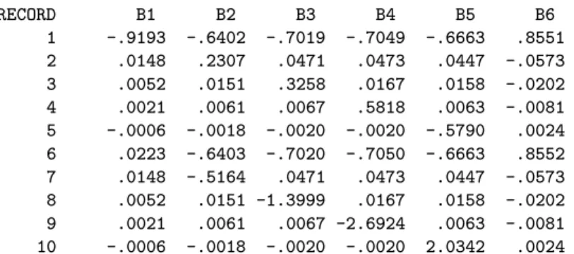
DELETION RESIDUALS OR APPROXIMATE CHANGE IN COEFFICIENTS AFTER DELETION OF EACH RECORD.

RECORD B1 B2 B3 B4 B5 B6 1 -.9193 -.6402 -.7019 -.7049 -.6663 .8551 2 .0148 .2307 .0471 .0473 .0447 -.0573 3 .0052 .0151 .3258 .0167 .0158 -.0202 4 .0021 .0061 .0067 .5818 .0063 -.0081 5 -.0006 -.0018 -.0020 -.0020 -.5790 .0024 6 .0223 -.6403 -.7020 -.7050 -.6663 .8552 7 .0148 -.5164 .0471 .0473 .0447 -.0573 8 .0052 .0151 -1.3999 .0167 .0158 -.0202 9 .0021 .0061 .0067 -2.6924 .0063 -.0081 10 -.0006 -.0018 -.0020 -.0020 2.0342 .0024

On the first page of the output, we see that the model is indeed additive, we also see the input data and the value of the deviance goodness of fit at each iteration. The number of observed and expected deaths are given and the Freeman-Tukey and Pearson residuals as well. At convergence, the coefficient for smoking (No. 6) is 0.5907. Thus, smoking adds 0.59 deaths per 1,000 person-years (or 59/100,000) of follow-up at each age. However, since theχ2 andDgoodness of fit statitics are greater then 4 degrees of freedom, we conclude that the model does not fit the data well. Table 6 shows the comparison between the modeled baseline rates and modeled baseline rates to which 0.59/1,000 was added.

Table 6: Interpretation of absolute risks from the additive model.

Baseline rate,_λ_i0(x0i0β) Smoker rate, λi1(x0i0β) (βj) (λi0(x0i0β) +βsmoke))

Age group,i per 1,000_T per 1,000_T

35-44 0.0841 0.6748

45-54 1.6407 2.2314

55-64 6.3035 6.8942

65-74 13.5241 14.115

75-84 19.1696 19.7603

Example 2: Multiplicative (log-linear) model using data in Table 1 adapted from [21]. The input data file for this run is the same as that in Example 1.

EXAMP1-3.DAT

(23)

EXPONENTIATE COEFFICIENTS? 0-NO 1-YES 1

The output file contains:

TITLE: PIRLS

MODEL SELECTED: MULTIPLICATIVE INPUT DATA FORMAT: (F4.0,F8.3,6F3.0)

ITERATION: 1 DEVIANCE: 53.9002

B COEFFICIENT STD. ERROR WALD SCORE

1 -1.0116 .1918 -5.2751 .00000207

2 .4724 .1304 3.6236 .00000969

3 1.6159 .1147 14.0944 -.00002298

4 2.3389 .1162 20.1343 .00001905

(24)

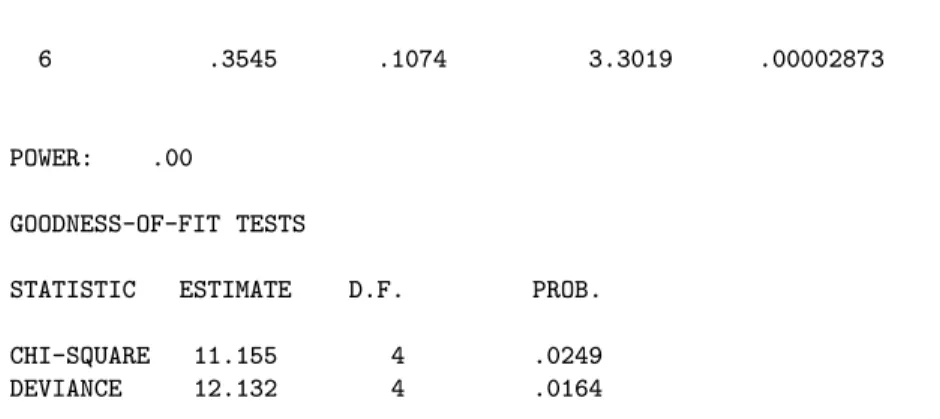
6 .3545 .1074 3.3019 .00002873

POWER: .00

GOODNESS-OF-FIT TESTS

CHI-SQUARE 11.155 4 .0249

DEVIANCE 12.132 4 .0164

At convergence, the coefficient for smoking (No. 6) is 0.3545. Since we exponentiated the regression coefficients, we can interpret the RR for smoking and the 95% confidence interval as being 1.43(1.15,1.76). This implies that the risk of coronary death in smokers is 1.43 times the age-specific rates of the non-smokers. The goodness of fit statistics for this run are greater than those generated in Example 1, indicating that the multiplicative model fits worse when compared with the additive model. Table 7 shows the comparison between modeled baseline rates and the modeled baseline rates multiplied by the RR of 1.43.

Table 7: Interpretation of relative risks from the multiplicative model.

Baseline rate,_λ_i0(x0i0β) Smoker rate, λ_i1(x0i0β)

(eβj₎ ₍_λ

i0(x0i0β)×eβsmoke))

35-44 0.36 0.5148

45-54 1.60 2.28

55-64 5.03 7.192

65-74 10.37 14.83

75-84 14.71 21.04

Example 3: Power model using data in Table 1 adapted from [21]. The input data file for this run is the same as that in Example 1.

EXAMP1-3.DAT

(25)

0

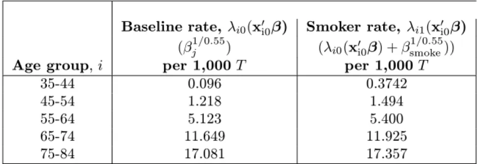
This run fitted ten models withρvarying from one to zero, i.e., going from a purely additive link,ρ= 1, to a purely multiplicative link,ρ= 0. The model quation isλi(x0_iβ)ρwhereρis the power function. By inspecting the fits of the models as a function ofρ, one can see that for these example data, the lowest deviance is obtained with ρbetween 0.5 to 0.6. A single run can now be made to fit the model with ρ= 0.55 by following the directions given in Example 1, but by specifying 0.55 forρinstead of one. Table 8 lists the modeled baseline rates,β_j1/0.55, and modeled baseline rates to whichβ_smoke1/0.55 was added.

Table 8: Interpretation of relative risks from the power model.

Baseline rate,_λ_i0(x0i0β) Smoker rate, λi1(x0i0β) (β1_j/0.55) (λi0(x0i0β) +β

1/0.55 smoke))

35-44 0.096 0.3742

45-54 1.218 1.494

55-64 5.123 5.400

65-74 11.649 11.925

75-84 17.081 17.357

Example 4: Non-linear model using cell concentrations, and radiation doses to estimate number of splenic stem cell colonies formed after transplantation into laboratory mice. The input data (see Table 4) for this run is provided in distribution file EXAMPLE4.DAT and is listed below:

Till and McCulloch (1961) (F4.0,F4.0,F7.2,F6.2) 60. 6. 1.25 .00 66. 7. 1.75 .96 46. 4. 3.00 1.92 82. 9. 7.20 2.88 105. 11. 24.00 4.32 123. 15. 75.00 5.76 12. 4. 120.00 6.72

EXAMPLE4.DAT

(26)

EXAMPLE4.OUT

INPUT OR ESTIMATE STARTING VALUES: 0-INPUT 1-EST 0

INPUT STARTING VALUE FOR COEFFICIENT: 1 7.6364

Results in the output file EXAMPLE4.OUT (filename specified above) indicate that 2 iterations were required before convergence was reached. Although the deviance and chi-square GOF values were greater than the 4 d.f., the Wald statistics for the parameters were statistically significant. The scores for all coefficients were near zero. The regression parameters, standard errors (with the exception of s.e.(β1)), correlation matrix, chi-square and deviance GOFs were identical to results in Frome [3].

TITLE: Till and McCulloch (1961) MODEL SELECTED: NON-LINEAR

INPUT DATA FORMAT: (F4.0,F4.0,F7.2,F6.2)

60. 6. 1.25 .00

66. 7. 1.75 .96

(27)

82. 9. 7.20 2.88 105. 11. 24.00 4.32 123. 15. 75.00 5.76

12. 4. 120.00 6.72

STARTING VALUES FOR PARAMETERS PARAMETER STARTING VALUE

1 7.6364000 2 .9341000 3 2.8924000 ITERATION: 1 DEVIANCE: 8.0174 ITERATION: 2 DEVIANCE: 8.0174 ITERATIONS: 2

REC OBS EXP FREEMAN-TUKEY PEARSON

1 60.0 57.3 .3874 .1298 2 66.0 73.0 -.8079 .6713 3 46.0 37.5 1.3496 1.9260 4 82.0 91.0 -.9414 .8942 5 105.0 101.4 .3807 .1296 6 123.0 113.9 .8536 .7194 7 12.0 19.9 -1.9041 3.1247

B COEFFICIENT STD. ERROR WALD SCORE

1 7.6364 .1186 64.3725 .00030114

2 .9341 .0399 23.4229 -.00096028

3 2.8924 .7476 3.8688 .00006890

POWER: .00

GOODNESS-OF-FIT TESTS

CHI-SQUARE 7.595 4 .1076

DEVIANCE 8.017 4 .0909

VARIANCE-COVARIANCE MATRIX OF COEFFICIENTS.

B1 B2 B3

B1 .014

(28)

B3 -.066 .025 .559

CORRELATION MATRIX OF COEFFICIENTS.

B1 B2 B3

B1 1.000

B2 -.343 1.000

B3 -.741 .853 1.000

TRACE OF THE HAT MATRIX AND ADJUSTED RESIDUALS.

RECORD LEVERAGE ADJ. RESID.

1 .8060 .8181 2 .3663 -1.0293 3 .2251 1.5766 4 .4551 -1.2811 5 .2954 .4289 6 .6358 1.4055 7 .2162 -1.9966

DELETION RESIDUALS OR APPROXIMATE CHANGE IN COEFFICIENTS AFTER DELETION OF EACH RECORD.

RECORD B1 B2 B3 1 -.1978 .0228 .9235 2 .0581 .0141 .0336 3 .0065 -.0276 -.4434 4 -.0339 .0336 .6643 5 .0060 -.0010 -.0749 6 -.0201 .0499 .4879 7 .0231 -.0354 -.4386