journal homepage:www.elsevier.com/locate/camwa
SAR image segmentation based on mixture context and wavelet
hidden-class-label Markov random field
IMing Li
a,∗, Yan Wu
b, Qiang Zhang
baNational Key Lab of Radar Signal Processing, Xidian University, Xi’an, 710071, China bSchool of Electronics Engineering, Xidian University, Xi’an, 710071, China
a r t i c l e i n f o
Keywords:
SAR image segmentation
Wavelet mixture heavy-tailed model Mixture context
Hidden-class-label MRF Overlapping window
a b s t r a c t
In order to suppress the effect of multiplicative speckle noise on Synthetic Aperture Radar (SAR) image segmentation, a new SAR image segmentation algorithm is proposed based on the mixture context and the wavelet hidden-class-label Markov Random Field (MRF). In our paper, a wavelet mixture heavy-tailed model is constructed, and the hidden-class-label MRF is extended to the wavelet domain to suppress the effect of speckle noise. The multiscale segmentation with overlapping window is presented here to segment the finest scale of stationary wavelet transform (SWT) domain, and the classical segmentation method is still utilized at the coarse scales of discrete wavelet transform (DWT) domain, moreover, a mixture context model is proposed to combine the two different segmentation methods. Finally, a new maximum a posteriori (MAP) classification is obtained. The experimental results demonstrate that our segmentation method outperforms several other segmentation methods.
©2008 Elsevier Ltd. All rights reserved. 1. Introduction
The segmentation of synthetic aperture radar (SAR) image is a key component in the automatic analysis and interpretation of data. Real SAR images are corrupted with an inherent signal-dependent phenomenon named multiplicative speckle noise, which is grainy in appearance and primarily due to the phase fluctuations of the electromagnetic return signals. Hence, the classical segmentation techniques that work successfully on natural images do not perform well on SAR images.
A Markov random field (MRF) is recognized to be a powerful stochastic tool used to model the joint probability distribution of the image pixels in terms of local spatial interactions [1,2]. MRF models can be used not only to extract texture features from image textures but also to model the image segmentation problem [2]. There are two advantages in using MRF models for image segmentation. First, the spatial relationship can be seamlessly integrated into a segmentation procedure. Second, the MRF-based segmentation model can be inferred in the Bayesian framework which is able to utilize different types of image features. There are various MRF-based segmentation models that have been developed [3–7]. The MRF-based segmentation method has also been applied to segment SAR images [8,9].
In multiscale segmentation [10,11] the results of many classification windows of different sizes are combined to obtain an accurate segmentation at fine scales. The wavelet transform can be interpreted as a multiscale edge detector that represents the singularity content of an image at multiple scales and three different orientations. Wavelets overlying a singularity yield
I This work was supported by the National Defence Foundation (9140A01060408DZ0104) and the National Natural Science Foundation of China (No. 60872137).
∗Corresponding author.
E-mail addresses:[email protected](M. Li),[email protected](Y. Wu),[email protected](Q. Zhang). 0898-1221/$ – see front matter©2008 Elsevier Ltd. All rights reserved.
(a) Texture 1. (b) Texture 2. (c) DWT wavelet coefficients of texture 1.
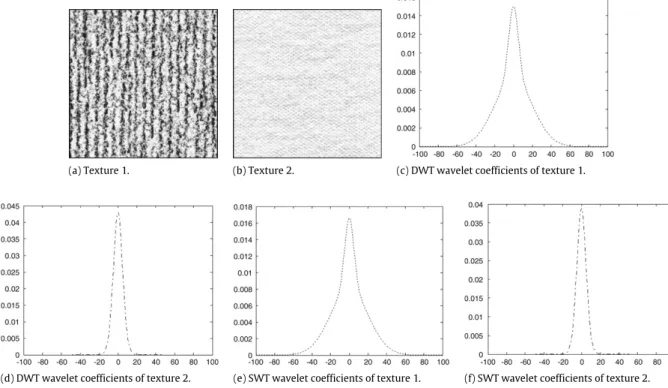
(d) DWT wavelet coefficients of texture 2. (e) SWT wavelet coefficients of texture 1. (f) SWT wavelet coefficients of texture 2. Fig. 1. Textures and heavy-tailed distributions of different wavelet coefficients in subband HH1.
large wavelet coefficients; wavelets overlying a smooth region yield small coefficients. Four wavelets at a given scale nest inside one at the next coarser scale, giving rise to a quad-tree structure of wavelet coefficients that mirrors that of the dyadic squares. In particular, with theHaar wavelet transform, each wavelet coefficient node in the wavelet quad-tree corresponds to a wavelet supported exactly on the corresponding dyadic image square.
Since the wavelet theory was developed and the Hidden Markov Model (HMM) which characterizes the statistics property of image was improved, the HMM segmentation based on the wavelet transform has been applied widely. Hyeokho Choi proposed the context segmentation algorithm based on the discrete wavelet transform (DWT) [12], which is utilized to natural image segmentation successfully, employing the results of coarse scales to influence that of fine scale. Later, based on the algorithm from Hyeokho Choi, Vidya Venkatachalam proposed SAR image segmentation algorithm [13], which trains and calculates coarse scales wavelet coefficients in the DWT domain to suppress speckle noise, however, the spatial resolution of segmentation result is reduced as well, so the problem of speckle noise is not solved perfectly. The Markov Random Filed (MRF) model has been employed to segment SAR image for a long time, because the local spatial dependency is considered in this algorithm, the speckle noise is suppressed effectively, However, the problem that this algorithm is just utilized in the image domain results in misclassification frequently. The application of Wavelet-Based MRF models to segment SAR image is not commonly represented in the research literature.
For SAR image segmentation, the segmentation algorithm is required not only to obtain accurate segmentation result but also to preserve detailed edge effectively. In order to solve these problems mentioned above, a new wavelet mixture heavy-tailed statistical model is presented in this paper, and the hidden-class-label MRF is extended to the wavelet domain to suppress the effect of speckle noise. The multiscale segmentation with overlapping block is proposed here, which is utilized at the finest scale of the stationary wavelet transform (SWT) domain to solve the problem of edge preservation, and the classical segmentation [14] is also utilized at coarse scales of the discrete wavelet transform (DWT) domain to solve the problem of reliable segmentation. In order to combine the two different segmentation algorithms, a mixture context is constructed, which fuses coarse scale segmentation results into fine scale result. Finally, the optimal segmentation result is derived from a new Maximum a Posteriori (MAP) classification. The variable local smoothness parameter is also employed in the Gibbs equation to improve estimate correctness. The experimental results show that the proposed algorithm decreases the effect of speckle noise and reduces misclassification phenomenon, and that it classifies SAR image more robustly and preserves edge more effectively.
2. Wavelet mixture heavy-tailed distribution model
Wavelet coefficients of SAR image present highly non-Gaussian statistical distribution [15]. As we see fromFig. 1(c) and (d), which exhibit the probability density distributions of DWT wavelet coefficients in subband HH1 for two texture samples shown inFig. 1(a) and (b) respectively, the non-Gaussian distribution is sharply peaked at zero and have extensive
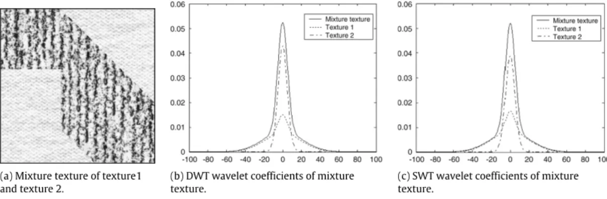
(a) Mixture texture of texture1 and texture 2.
(b) DWT wavelet coefficients of mixture texture.
(c) SWT wavelet coefficients of mixture texture.
Fig. 2. Mixture texture and mixture heavy-tailed distributions of two different wavelet coefficients in subband HH1.
tails, so called heavy-tailed distribution.Fig. 1(e) and (f) show that the probability density distribution of SWT wavelet coefficients is similar to that of DWT wavelet coefficients, thus a same symbol
w
is used to denote the DWT and SWT wavelet coefficient. We assume each wavelet coefficient is composed of two states [16,17], and the probability distribution for each state is Gaussian distribution: ‘‘high’’ indicated withs0, representing coefficients with large signal energy, corresponds tothe Gaussian distribution with zero mean and high variance
σ
02; ‘‘low’’ indicated withs1, representing coefficients with littlesignal energy, corresponds to the Gaussian distribution with zero mean and low variance
σ
21. So the mixture probability
density function (pdf) of the wavelet coefficient is defined as
f
(w)
=
X
m=0,1
p
(
s=
m)
p(w
|
s=
m)
(1)wherep
(w
|
s=
m)
∼
N(
0, σ
2wm
)
.p(
s=
m)
stands for the probability mass function (pmf) of statem, andp(
s=
0)
+
p(
s=
1)
=
1.Suppose that an image is composed ofNdifferent textures, andcindicates the class label,c
=
1,
2, . . . ,
N. The pdf of the given image is the mixture of the pdfs ofNdifferent classes. Because the wavelet transform is linear, the pdf of the given image wavelet coefficients is also regarded as the mixture of the pdfs ofNdifferent classes wavelet coefficients. The probability density distribution of each class wavelet coefficients shows the heavy-tailed distribution, so the probability density distribution of the given image wavelet coefficients presents the mixture heavy-tailed distribution. Thus, the pdf of the given image wavelet coefficients is defined asfseg
(w)
=
NX
k=1
p
(
c=
k)
f(w
|
c=
k)
(2)wheref
(w
|
c=
k)
stands for the conditional pdf of classkwavelet coefficients, which is the mixture pdf with two states mentioned above,p(
c=
k)
denotes the pmf of classk.Fig. 2(b) and (c) show the probability density distributions of two different wavelet coefficients in subband HH1 for the mixture texture shown inFig. 2(a). These two figures demonstrate that no matter in the DWT domain or in the SWT domain the probability density distribution of the mixture texture image wavelet coefficients is the mixture of the probability density distributions of the two textures wavelet coefficients according to their pmfs.3. Wavelet hidden-class-label MRF segmentation based on mixture context
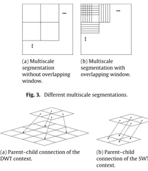
Multiscale segmentation uses different size of classification window to segment image [18], which captures pixel statistical information from a same window to estimate class label and makes all pixels in the window belong to the same class. Because more pixels provide more rich statistical information, larger window produces more accurate segmentation results in large and homogeneous regions, but poor segmentations along the boundaries between regions. The window in the classical multiscale segmentation is not overlapping, as shown inFig. 3(a), but this property makes the pixels on the margin of the window misclassified. So a new segmentation method with overlapping window (shown inFig. 3(b)) is proposed here, the overlapping window sites the segmented pixel at the center of the window to estimate the class label of the pixel more accurately, furthermore, detailed edges are preserved effectively.
3.1. Raw segmentation in the wavelet domain
First of all, we train wavelet coefficients of each representative texture using the iterative expectation–maximization (EM) algorithm [19], then obtain the parameterpsi
(
m)
, the meanµ
i,mand the varianceσ
2
i,m, whereistands for theith wavelet coefficient,m
=
0,
1. These parameters can be grouped into a parameter vectorΘ, whereΘ=
psi(
m), µ
i,m, σ
2 i,m .
window.
Fig. 3. Different multiscale segmentations.
(a) Parent–child connection of the DWT context.
(b) Parent–child connection of the SWT context.
Fig. 4. Two different parent–child connections. The direction of arrow is from parent to child.
A complete 2D image wavelet transform comprises three subbands: HH, HL and LH. Denoting these parameter vectors for the three subbands asΘHH,ΘHLandΘLHrespectively, we haveM
= {
ΘHH,
ΘHL,
ΘLH}
. While the three subbands are dependent on each other, for tractability reason, we assume that they are statistically independent. So the joint pdf of the wavelet coefficients as follow:f
(w
|
M)
=
f(w
HH|
ΘHH)
f(w
HL|
ΘHL)
f(w
LH|
ΘLH).
(3) Suppose that an image includesNdifferent classes,c∈ {
1,
2, . . . ,
N}
, and the functionf(w
i|
Mc)
is obtained, the raw segmentation function is derived from the simplest ML classification and(3).ˆ
ciML
=
arg max c∈{1,2,...,N}f(w
i|
Mc).
(4)In what follows,f
(w
|
c)
stands forf(w
|
Mc)
for short.3.2. Mixture context model
In order to apply the multiscale segmentation with overlapping window, the SWT is employed in this paper, the decomposed result by which has the same size as original image, but the SWT is a redundant transform, especially at the coarse scale the original image cannot be described with SWT wavelet coefficients very well, so the SWT decomposition is only utilized at the finest scale. Other scales wavelet coefficients are obtained by the DWT decomposition, which is used to perform the classical multiscale segmentation. For the two different multiscale segmentations, two corresponding context models are employed to fuse the segmentation results of different scales. In the DWT context model, each child has just one parent, but each parent has four children, as shown inFig. 4(a). In the SWT context model, child and its parent are one-to-one mapping, as shown inFig. 4(b). Since it is not reliable enough that child class label is decided just by its parent, the combination of the parent and its appropriate neighbors is necessary. In our paper, the neighbors are defined as parent’s eight neighbors in the SWT context and the parents of child’s neighbors in the DWT context.
In order to express the positions of these neighbors in the DWT context, we denote a wavelet coefficient at scalejas
l
=
(
x,
y)
, wherexandyare the row and column indices respectively. The neighbors at scalej+
1 in the DWT context isl1
=
(
b
x/
2c
,
b
y/
2c
)
l2
=
(
b
x/
2c
,
b
y/
2c
)
+
(
even(
x),
0)
l3=
(
b
x/
2c
,
b
y/
2c
)
+
(
0,
even(
y))
l4=
(
b
x/
2c
,
b
y/
2c
)
+
(
even(
x),
even(
y))
(5)
where ifxis even, even
(
x)
=
1; andxis odd, even(
x)
= −
1. Theb·c
function rounds the argument to the nearest integer towards minus infinity.The neighbor decision denoted as
v
lis the majority vote of the class labels of these neighbors, so the class label of wavelet coefficientw
lis affected by two factors: its parent class labelcp(i)and its neighbor decisionv
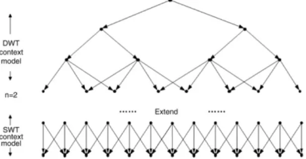
l. Thus, the class transitionFig. 5. 1D analog to the mixture context model. Each black node denotes a wavelet coefficient, arrow denotes dependency.
probability is denoted asp
(
ci|
cp(i), v
i)
, which represents the conditional probability for the class labelci, when the parent class label iscp(i)and the neighbor decision isv
i, wherep(
i)
stands for the parent of notei. By Bayes rule,p(
ci|
cp(i), v
i)
is given byp
(
ci|
cp(i), v
i)
=
p
(
cp(i), v
i|
ci)
p(
ci)
p
(
cp(i), v
i)
.
(6) An iterative EM algorithm [12] is employed to calculate the unknown parameters.Fig. 5shows the mixture context model in our algorithm. When the scale leveln
>
2, the DWT context is used to estimate the interscale class transition probability, when the scale leveln≤
2, the SWT context is used.3.3. Hidden-class-label MRF and new map classification
The context fuses the segmentation results from coarse scale to fine scale to reduce misclassification, but it cannot suppress the effect of multiplicative speckle noise in SAR image. In this paper, the hidden-class-label MRF [19] is employed to estimate prior probability, where the class labelcis hidden state. In this method, the clustering of wavelet coefficient is taken into account, which results in that the prior probability of wavelet coefficient is estimated depending on its intrascale neighbors’ class labels, so the effect of speckle noise is decreased.
In order to distinguish from the priorp
(
ci|
cp(i), v
i)
defined in previous section, the new priorpnew(
ci|
cp(i), v
i)
is employed, which is derived from the MRF. Moreover, only single-site and pair-site cliques are adopted here. Because a Gibbs Random Field (GRF) is a MRF [19], we choose the joint probability distribution over the random field represented by GRF. So the prior is defined as a GRF. pnew(
c|
cp, v)
=
1 Ze −U(c|cp,v) (7) U(
c|
cp, v)
=
V1(
c|
cp, v)
+
V2(
c|
cp, v)
(8) e−V1(c|cp,v)=
MY
i=1 p(
ci|
cp(i), v
i)
(9) V2(
c|
cp, v)
= −
β
MX
i=1X
j∈η(i)(δ(
ci−
cj)
−
1)
(10)where Z is a normalizing constant;
β
is the parameter that controls the local smoothness;η(
i)
is the second-order neighborhood of pixeli;
δ(
·
)
is the discrete delta function; V1 and V2 are the single-site and pair-site clique functionrespectively.
We assume that functionf
(w
|
c)
and priorpnew(
c|
cp, v)
is known, according to the MAP and the Bayes rule, the optimal classification is given byˆ
c
=
arg maxp(
c|
w
,cp, v)
=
arg maxf(w
|
c)
pnew(
c|
cp, v).
(11)The local conditional probability equation is derived from GRF model shown in(7)–(10).
p
(
ci|
cp(i), v
i,
cη(i))
=
1 Z0p(
ci|
cp(i), v
i)
×
exp 2β
X
j∈η(i)(δ(
ci−
cj)
−
1)
!
(12)we generate the initial class labelci based on priorp
(
cicp(i), v
i)
and the MAP criterion.ˆ
ci0=
arg max ci∈{1,2,...,N} p(
ci|
w
i,
cp(i), v
i)
=
arg max ci∈{1,2,...,N} f(w
i|
ci)
p(
ci|
cp(i), v
i).
(14) In former literatures, the parameterβ
is a constant, which has some disadvantages. If the constant parameter makes the local dependency dominant, the estimated parameters may deviate from the real values; if the constant parameter makesf
(w
|
c)
and the interscale transition probability dominant, the local dependency would be ignored in the final segmentation result. So the varianceβ
is utilized in this paper, which can balance weights of the two components mentioned above during segmentation.β(
i)
=
1c1
×
rI+
c2(15) where 0
<
r<
1,r,
c1andc2are constant,Istands for theIth iteration. Here, we assumer=
0.
95,
c1=
80,
c2=
1. 3.4. Pixel-level segmentationThe probability density distribution of each texture in the image domain is modeled by its histogram, so we assume that each texture corresponds to the Gaussian distribution, and that the image to be segmented corresponds to the mixture Gaussian distribution. During pixel-level segmentation, the SWT context is employed to estimate the interscale class transition probability and the hidden-class-label MRF is utilized to characterize the dependencies between pixels.
The proposed segmentation algorithm
1. Decompose samples and the image to be segmented at the finest scale using the SWT and the other coarse scales using the DWT, then train samples using EM algorithm to obtain the conditional pdff
(w
|
c)
.2. Apply raw segmentation at the coarsest scale.
3. Segment next finer scale, computep
(
ci|
cp(i), v
i)
using the upper scale result and the DWT context.4. Calculate initial class labels, iterate the new MAP classification to obtain the optimal segmentation result of this scale. 5. Repeat step 3 from 4 until the second scale level.
6. Extend the second scale level to the size of original image, employ the SWT context to estimatep
(
ci|
cp(i), v
i)
at the finest scale, and obtain the optimal result by iterating the new MAP classification.7. Apply the pixel-level segmentation using the finest scale result.
The multiscale segmentation with overlapping window is also proposed here, which is utilized at the finest scale of the stationary wavelet transform (SWT) domain to solve the problem of edge preservation, and the classical segmentation is also utilized at coarse scales of the discrete wavelet transform (DWT) domain to solve the problem of reliable segmentation. In order to combine the two different segmentation algorithms, a mixture context is constructed, which fuses coarse scale segmentation results into fine scale result.
4. Experimental results and discussion
In this section, the proposed algorithm is tested on two 128
×
128 and two 512×
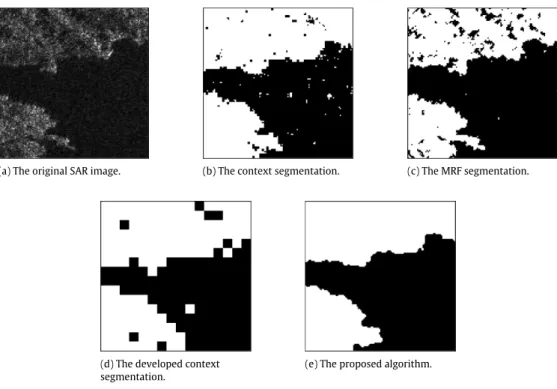
512 real SAR images (shown inFigs. 6(a) and7(a),8(a) and9(a)). Because the segmentation algorithm [13] proposed by Vidya Venkatachalam has the ability to suppress the effect of speckle noise in SAR image, we select it in the comparison and name it the developed context segmentation. The other algorithms include the following: the context segmentation and the MRF segmentation, which are mentioned in the introduction. Both of the proposed algorithm and the context segmentation algorithm are pixel-level segmentation, and the developed context segmentation algorithm is 8
×
8 block segmentation. The mother wavelet is Haar here, and the number of decomposition level is 4. InFigs. 6(b) and7(b),8(b) and9(b), because the context segmentation fuses all the scales results into final result, large and homogeneous regions are classified accurately, but this algorithm cannot suppress the effect of speckle noise effectively, plenty of granular-misclassification points appear in the segmented results. The MRF segmentation employs the intrascale local dependency to reduce the effect of speckle noise, but this algorithm is applied in the image domain, the global information is ignored, as illustrated fromFigs. 6(c) and7(c),8(c) and9(c), the(a) The original SAR image. (b) The context segmentation. (c) The MRF segmentation.
(d) The developed context segmentation.
(e) The proposed algorithm.
Fig. 6. Comparison of the different segmentation algorithms.
(a) The original SAR image. (b) The context segmentation. (c) The MRF segmentation.
(d) The developed context segmentation.
(e) The proposed algorithm.
Fig. 7. Comparison of the different segmentation algorithms.
granular-misclassification point is removed obviously, however, these parts of the homogeneous region, the textures of which are similar to other textures, are always misclassified. The developed context segmentation (shown inFigs. 6(d) and
7(d),8(d) and9(d)) is able to suppress the effect of speckle noise, but the spatial resolution of the segmented result is poor. In our algorithm, the intrascale local spatial dependency at each scale is considered and all scales segmentation results is fused into final result, so the granular-misclassification point is suppressed and the misclassification in homogeneous region is reduced, furthermore, the segmentation at the finest scale of the SWT domain makes detailed edges more obvious.
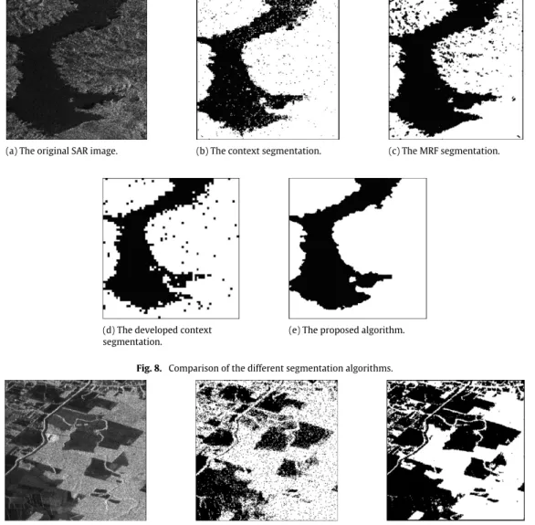
(a) The original SAR image. (b) The context segmentation. (c) The MRF segmentation.
(d) The developed context segmentation.
(e) The proposed algorithm.
Fig. 8. Comparison of the different segmentation algorithms.
(a) The original SAR image. (b) The context segmentation. (c) The MRF segmentation.
(d) The developed context segmentation.
(e) The proposed algorithm.
Fig. 9. Comparison of the different segmentation algorithms.
of homogeneous regions are accurate, granular-misclassification points are decreased, and detailed edges are successfully preserved. Compared with the other ones, the segmented results have better visual effect.
5. Conclusions
By constructing the wavelet mixture heavy-tailed model of the image to be segmented, the new segmentation algorithm was proposed in this paper based on the mixture context model and the hidden-class-label MRF. The class label was
References
[1] S. Geman, D. Geman, Stochastic relaxation, Gibbs distributions, and the Bayesian restoration of images, IEEE Trans. Pattern Anal. Mach. Intell. PAMI-6 (6) (1984) 721–741.
[2] S.Z. Li, Markov Random Field Modeling in Computer Vision, Springer-Verlag, New York, 2001.
[3] F.S. Cohen, D.B. Cooper, Simple parallel hierarchical and relaxation algorithms for segmenting noncausal Markovian random fields, IEEE Trans. Pattern Anal. Mach. Intell. PAMI-9 (2) (1987) 195–219.
[4] C.S. Won, H. Derin, Unsupervised segmentation of noisy and textured images using Markov random fields, Graph. Models Image Process. 54 (4) (1992) 308–328.
[5] D.K. Panjwani, G. Healey, Markov random field models for unsupervised segmentation of textured color images, IEEE Trans. Pattern Anal. Mach. Intell 17 (10) (1995) 939–954.
[6] S.A. Barker, Image segmentation using Markov random field models, Ph.D. Dissertation, Cambridge Univ., Cambridge, UK, 1998.
[7] P.A. Kelly, H. Derin, K.D. Hartt, Adaptive segmentation of specked images using a hierarchical random field model, IEEE Trans. Acoust. Speech Signal Process. 36 (10) (1988) 1628–1641.
[8] Deng Huawu, D.A. Clausi, Unsupervised segmentation of synthetic aperture radar sea ice imagery using a novel markov random field model, IEEE Trans. Geosci. Remote. Sens. 43 (3) (2005) 528–538.
[9] O. Lankoande, M.M. Hayat, Santhanam Balu, Segmentation of SAR images based on markov random field model, in: System, Man and Cybernetics, 2005 IEEE International Conference, 2005, pp. 2956–2961.
[10] C. Fosgate, H. Krim, W. Irving, W. Karl, A. Willsky, Multiscale segmentation and anomaly enhancement of SAR imagery, IEEE Trans. Image Process. 6 (1997) 7–20.
[11] J. Li, R.M. Gray, R.A. Olshen, Multiscale image classification by hierarchical modeling with two dimensional hidden Markov models, IEEE Trans. Inform. Theory 46 (5) (2000) 1826–1841.
[12] H. Choi, R.G. Baraniuk, Multiscale image segmentation using wavelet-domain hidden markov models, IEEE Trans. Image Process. 10 (9) (2001) 1309–1321.
[13] V. Venkatachalam, H. Choi, R.G. Baraniuk, Multiscale SAR image segmentation using wavelet domain hidden markov tree models, in: Proc. SPIE-The International Society for Optical Engineering, vol. 4053, 2000, pp. 110–120.
[14] C.A. Bouman, M.A. Shapiro, Multiscale random field model for Bayesian image segmentation, IEEE Trans. Image Process. 3 (2) (1994) 162–177. [15] S.G. Mallat, A theory for multiresolution signal decomposition: The wavelet representation, IEEE Trans. Pattern Anal. Machine Intell. 11 (7) (1989)
674–693.
[16] M.S. Crouse, R.D. Nowak, R.G. Baraniuk, Wavelet-based statistical signal processing using hidden markov models, IEEE Trans. Signal Processing 46 (4) (1998) 886–902.
[17] C. Fosgate, H. Krim, W. Irving, W. Karl, A. Willsky, Multiscale segmentation and anomaly enhancement of SAR imagery, IEEE Trans. Image Processing 6 (1997) 7–20.
[18] Xie Hua, L.E. Pierce, F.T. Ulaby, Sar speckle reduction using wavelet denoising and markov random field modeling, IEEE Trans. Geosci. Remote Sens. 40 (10) (2002) 2196–2212.