Master’s Programme in Computer Science
Incomplete MaxSAT Solving by Linear
Programming Relaxation and Rounding
Esa Kemppainen
June 8, 2020
Faculty of Science
University of Helsinki
Supervisor(s)
Assoc. Prof. Matti J¨arvisalo, Dr. Jeremias Berg Examiner(s)
Assoc. Prof. Matti J¨arvisalo, Dr. Jeremias Berg
Contact information
P. O. Box 68 (Pietari Kalmin katu 5) 00014 University of Helsinki,Finland
Email address: [email protected] URL: http://www.cs.helsinki.fi/
Faculty of Science Master’s Programme in Computer Science Esa Kemppainen
Incomplete MaxSAT Solving by Linear Programming Relaxation and Rounding Assoc. Prof. Matti J¨arvisalo, Dr. Jeremias Berg
MSc thesis June 8, 2020 57 pages
maximum satisfiability, linear programming, combinatorial optimization Helsinki University Library
Algorithms study track
NP-hard optimization problems can be found in various real-world settings such as scheduling, planning and data analysis. Coming up with algorithms that can efficiently solve these prob-lems can save various rescources. Instead of developing problem domain specific algorithms we can encode a problem instance as an instance of maximum satisfiability (MaxSAT), which is an optimization extension of Boolean satisfiability (SAT). We can then solve instances result-ing from this encodresult-ing usresult-ing MaxSAT specific algorithms. This way we can solve instances in various different problem domains by focusing on developing algorithms to solve MaxSAT instances.
Computing an optimal solution and proving optimality of the found solution can be time-consuming in real-world settings. Finding an optimal solution for problems in these settings is often not feasible. Instead we are only interested in finding a good quality solution fast. Incomplete solvers trade guaranteed optimality for better scalability.
In this thesis, we study an incomplete solution approach for solving MaxSAT based on linear programming relaxation and rounding. Linear programming (LP) relaxation and rounding has been used for obtaining approximation algorithms on various NP-hard optimization problems. As such we are interested in investigating the effectiveness of this approach on MaxSAT. We describe multiple rounding heuristics that are empirically evaluated on random, crafted and industrial MaxSAT instances from yearly MaxSAT Evaluations. We compare rounding ap-proaches against each other and to state-of-the-art incomplete solvers SATLike and Loandra. The LP relaxation based rounding approaches are not competitive in general against either SATLike or Loandra However, for some problem domains our approach manages to be compet-itive against SATLike and Loandra.
ACM Computing Classification System (CCS)
Mathematics of computing →Discrete mathematics→Combinatorics
Tekij¨a — F¨orfattare — Author
Ty¨on nimi — Arbetets titel — Title
Ohjaajat — Handledare — Supervisors
Ty¨on laji — Arbetets art — Level Aika — Datum — Month and year Sivum¨a¨ar¨a — Sidoantal — Number of pages
Tiivistelm¨a — Referat — Abstract
Avainsanat — Nyckelord — Keywords
S¨ailytyspaikka — F¨orvaringsst¨alle — Where deposited
1 Introduction 1 2 Maximum Satisfiability 4 2.1 Boolean Satisfiability . . . 4 2.2 MaxSAT . . . 6 2.3 MaxSAT Solving . . . 9 2.3.1 Complete Algorithms . . . 9 2.3.2 Incomplete Algorithms . . . 10
2.3.3 MaxSAT With ILP . . . 13
3 Linear Programming 14 3.1 Linear Programming Definitions . . . 14
3.2 Integer Linear Programming Definitions . . . 16
3.3 LP Relaxation and Approximations . . . 17
3.4 ILP Solving . . . 21
3.5 LP Solving . . . 22
4 LP Relaxations for Incomplete MaxSAT Solving 24 4.1 Encoding MaxSAT to ILP . . . 24
4.2 Rounding LP Relaxations for MaxSAT . . . 25
4.2.1 Threshold Rounding . . . 27
4.2.2 Iterative Rounding . . . 29
4.3 Implementation . . . 32
5 Experiments 34 5.1 Evaluation Setup . . . 34
5.2 Comparing Different Rounding Methods . . . 35
5.3 LP Relaxation Solution Analysis . . . 40
5.5 Results for Partial MaxSAT Instances . . . 45
6 Conclusions 47
In real-world settings we are often confronted with the task of finding the best possible solution to a problem with a time limit. Such problems are called optimization problems. Oftentimes interesting optimization problems are NP-hard. If the solution space for an optimization problem is discrete we call it a combinatorial optimization problem [88]. NP-hard combinatorial optimization problems arise for example in planning [63], scheduling [75, 17], bioinformatics [46] and data analysis [14]. Algorithms that compute low cost solutions to these problems can save money, time and various kinds of various kinds of other resources. Therefore, there is lot of interest in developing algorithms that can be used to solve NP-hard optimization problems efficiently. In this thesis we develop an incomplete solution approach based on the so-called declarative paradigm for solving combinatorial optimization problems.
Solution approaches for combinatorial optimization problems can be divided into com-plete and incomcom-plete approaches. Given enough resources, the comcom-plete approaches find an optimal solution to a problem and prove its optimality These can be further divided into problem-specific exact algorithms [12] and exact declarative methods [91]. Problem-specific exact algorithms are algorithms developed for finding an optimal solution for instances in a specific problem domain. Exact declarative methods offer a way to solve instances from different problem domains. This is done by encoding a problem instance into a constraint language for which there exists an efficient solver. A declarative solver is an implementation of an algorithm designed for solving instances of constraint optimiza-tion problems for specific constraint languages. Examples of commonly used constraint optimization problems are maximum satisfiability (MaxSAT) [70] and integer linear pro-gramming (ILP) [27, 25] both of which we detail in this thesis. Solutions for the instances resulting from encoding can be then decoded back to solutions for the original problem instance.
MaxSAT is an optimization extension of the well-known NP-complete problem known as Boolean satisfiability, or SAT [24]. The underlying constraint language used by MaxSAT is conjunctive normal form (CNF) formulas. Once a problem instance is encoded as a CNF formula, we can use a MaxSAT solver to obtain a solution for the encoding. Many different approaches have been proposed for MaxSAT solving [66, 64, 35, 5, 78, 92, 30, 13].
2
The most important one for this work is to encode MaxSAT as integer linear programming (ILP) [6]. ILP is also an exact declarative method used to solve combinatorial optimization problems. ILP uses linear inequalities as the underlying constraint language.
In contrast to complete solution approaches, incomplete solution approaches are designed to give the best found solution within a given time limit without guaranteeing the opti-mality. Unless P = NP, no complete approach is not going to be effective on all instances of an NP-hard optimization problem. Furthermore, in many real-world applications, we are more interested in finding a good quality solution efficiently than finding an optimal solution. As such there is an interest in developing incomplete approaches since they scale better with real-world applications by sacrificing the guarantee of finding an opti-mal solution. Incomplete approaches can be further roughly divided into two categories; approximation algorithms [103, 47, 102] and local search algorithms [50]. A local search algorithm finds a solution and tries to improve the already found solution by searching the neighboring search space. Approximation algorithms obtain solutions for NP-hard problems efficiently and the obtained solution is guaranteed to be a certain factor away from an optimal solution.
One commonly used approximation algorithm for ILP is based on using linear program-ming (LP) relaxation [89, 53] and rounding. Similarly to ILP, LP is a declarative method based on linear inequalities. The main difference between these two is that compared to ILP, LP does not have integrality constraints over variables which makes LP polynomial-time solvable [61]. The LP relaxation on an ILP instance creates a related LP instance with same linear inequality constraints but with the integrality constraint removed. Solv-ing this related LP instance and roundSolv-ing the solution to have integer values can create an approximation algorithm for the original ILP instance. Using LP relaxations and round-ing is a well-studied approach on obtainround-ing a solution for NP-hard optimization problems [23, 19, 2]. However, using LP relaxations and rounding to solve MaxSAT instances en-coded as ILP has not gained as much attention, even if similar relaxation approaches using semidefinite programming (SDP) [40] and SDP relaxation have shown promising results on a special case of MaxSAT known as MAX-2-SAT [42] where each clause is restricted to have exactly two variables. In the referred work it was shown that good quality lower and upper bounds for optimal solutions could be found within seconds by using SDP re-laxations. LP relaxations have also been shown to be effective on MAX-2-SAT in [57] and have been used to improve a complete solver by obtaining lower bounds for MAX-2-SAT and MAX-3-SAT instances [105]. In contrast to these works, we explore using an LP
re-laxation approach with rounding for the general MaxSAT problem where clauses have no restrictions on number of variables. Furthermore, we empirically evaluate the approaches using crafted and industrial benchmark instances in addition to random instances. More specifically we investigate the quality of solutions obtained by using LP relaxations and rounding to solve MaxSAT instances. We describe multiple different rounding heuris-tics and empirically evaluate them by running them on MaxSAT instances used in MaxSAT Evaluations [10, 9]. We show that there are differences between rounding approaches. We also show that our approach manages to obtain good solutions on some problem domains fornon-partial MaxSAT instances when compared to state-of-the-art solvers.
This thesis is organized as follows. In Chapter 2 we go over the definitions of MaxSAT and give an overview of approaches used to solve MaxSAT instances. In Chapter 3 we go over the definitions of ILP and LP, discuss what LP relaxation is and give an overview of central approaches to solve ILP and LP instances. In Chapter 4 we describe how to encode MaxSAT problems into ILP instances and further into LP, discuss different rounding heuristics considered in this thesis and discuss how these approaches were implemented. In Chapter 5 we present results from our empirical evaluation by comparing the considered rounding heuristics against each other and against state-of-the-art incomplete MaxSAT solvers. Chapter 6 concludes this thesis and discusses possible future work.
2 Maximum Satisfiability
As our goal is to develop an approach for solving maximum satisfiability (MaxSAT) we start by defining concepts related to MaxSAT. Firstly in Section 2.1 we define what the Boolean satsifiability problem is. In Section 2.2 we define the MaxSAT problem. Lastly in Section 2.3 we review algorithmic approaches that are used to solve MaxSAT instances.
2.1
Boolean Satisfiability
Boolean satisfiability [34], or SAT for short, is the problem of determining whether a given propositional formula is satisfiable or not. This is a well-known NP-complete prob-lem [24]. Propositional formulas consist of atomic propositions and logical operators. A propositional formulas in conjunctive normal formal, or CNF for short, are constructed as follows.
• A literal l is either a Boolean variable x or its negation ¬x.
• A clause C of lengthm is is a disjunction l1∨. . .∨lm of literals.
• A CNF formula F with k clauses is a conjunction C1∧. . .∧Ck.
Any propositional logic formula can be transformed into CNF without loss of generality. This can be done so that the size of the resulting formula is linear in the size of the original formula in a standard way using the so-called Tseitin encoding [101]. A truth assignment τ sets each literal to either true or false. More formally, given a set of Boolean variables V, a truth assignment τ is a mappingτ :V → {0,1}, where zero corresponds to false and one to true. For a CNF formula to evaluate to true at least one literal in each clause needs to be satisfied by a truth assignment. More precisely:
• A literall is satisfied byτ, ifl is a Boolean variablexand τ(x) = 1 or ifl is negated variable ¬x and τ(x) = 0.
• A clause C =l1∨. . .∨ln is satisfied byτ, if τ(lk) = 1 for some 1, . . . , n.
Since a CNF formula consists of clauses that are connected by conjunctions, we can view a CNF formula F =C1∧. . .∧Ck as a set of clauses F ={C1, . . . , Ck}.
A SAT solver [76] is a program that, given a CNF formula F as an input, decides if the formula F have a satisfying truth assignment. Advances in SAT solvers has made them competitive in solving computationally hard problems [54, 90]. Instead of having to come up with specific algorithm for some decision problem we can encode the problem to a CNF formula and then use a SAT solver to solve the SAT instance. If a solution for the SAT instance exists, a SAT solver can return the solution for the instance which can be mapped back to a solution for the original problem instance.
Example 1 The k-coloring is a problem, where given a graph G= (V, E) and an integer
k, the goal is to decide if each of the vertices can be colored so that no adjacent vertices have the same color assigned using k colors. This problem can be encoded into SAT as follows.
A variablexv,i corresponds to a vertex v that has been assigned a color i. For each vertex
and for each i, where 1≤i≤k, we create the following clauses.
k
_
i=1
xv,i
To enforce that there is only one color assigned to each vertexv ∈V we create the following constraints. k−1 ^ i=1 k ^ j=i+1 (¬xv,i∨ ¬xv,j)
To enforce that, for each edge (v, u) ∈ E, vertices v and u cannot have the same color assigned we create the following constraints.
k
^
i=1
(¬xv,i ∨ ¬xu,i)
If the propositional formula consisting of these clauses is satisfiable, then there is an as-signing of colors that colors the given graphG. If the propositional formula is unsatisfiable, then there is no assigning of colors that colors the given graphG.
6
2.2
MaxSAT
Maximum satisfiablity, or MaxSAT [70], is an optimization extension of the Boolean sat-isfiability problem. Whereas the goal in the Boolean satsat-isfiability problem is to decide if a given Boolean formula is satisfiable, in MaxSAT the goal is to find a truth assignment that maximizes the number of satisfied clauses in a given Boolean formula. For some intuition let us consider the following example.
Example 2 Let F be the CNF formula
(x)∧(x∨y)∧(¬x∨y)∧(x∨ ¬y)∧(¬x∨ ¬y).
This formula is unsatisfiable. However, different truth assignments satisfy different num-bers of clauses. If for example we set x to false then we can satisfy at most three clauses. On the other hand, if we set x to true, then we can satisfy four clauses as x= 1 satisfies clauses (x),(x∨y) and (x∨ ¬y), and the remaining clauses (¬x∨y) and (¬x∨ ¬y) can be satisfied by either setting y to true or to false.
The formulaF in Example 2 is anon-partial MaxSAT instance. This means that there are
no requirements on which clauses must be satisfied. However, in many practical problems we usually have some constraints that must be satisfied. In other words, when encoding a problem to MaxSAT we would want to force certain clauses to be true in all solutions. A partial MaxSAT instance may also contain clauses that must be satisfied. These types
of clauses are called hard clauses. Clauses that do not have to be satisfied are called soft clauses.
Definition 1 Let F be a partial MaxSAT instance F = {Fh, Fs}, where Fh is a set of
hard clauses and Fs is a set of soft clauses. A solution for F is a truth assignment that
satisfies all hard clauses of F.
Non-partial can be seen as a special case where the set of hard clauses is empty. Hence,
by the definition, any truth assignment for a non-partial MaxSAT instance is a solution.
Fh ={(x∨y),(x∨z),(x∨ ¬y),(¬x∨ ¬y)} and
Fs ={(x),(y),(z)}.
Here a truth assignment τ that sets x, y and z to true would not be a solution as it would not satisfy the hard clause (¬x∨ ¬y). On the other hand, a truth assignment τ0 that sets x and z to true and y to not true would be a solution.
Furthermore, weights can be associated with soft clauses of MaxSAT instances. These types of instances are called weighted MaxSAT instances. Hard clauses have no assigned weights as they need to be satisfied by a truth assignment for it to be a solution. If all the weights of a MaxSAT instance are one, we call the instance an unweighted MaxSAT instance. The cost of a solution is defined as follows.
Definition 2 Given a weighted MaxSAT instance F and a truth assignment τ, the cost of τ is the sum of all weights of the soft clauses of the F not satisfied by τ. More formally cost(F, τ) = P
C∈Fs
w(C)·(1−τ(C)).
Definition 3 Let F be a MaxSAT formula. An optimal solution for F is a solution that has the smallest cost of all solutions.
Now we can define the MaxSAT problem as finding a solution for a MaxSAT instance F that has the smallest cost over all solutions forF. With these definitions let us consider the following example.
Example 4 Let F be a MaxSAT formula F ={Fh, Fs}, where
Fh ={(x∨y),(x∨z),(x∨ ¬y),(¬x∨ ¬y)} and
Fs ={(x,3),(y,2),(z,5)}.
Here a truth assignment τ that sets x to true and y and z to false has cost(F, τ) = 7. While this is a solution forF it is not optimal. An optimal solution τ0sets xand z to true and y to false and has cost(F, τ0) = 2.
8
To give an example on how to encode a problem in MaxSAT let us consider the graph coloring problem already discussed in the previous section.
Example 5 In the optimization variant of the problem presented in Example 1, the goal is to find a minimum number of colors to color a given graph G = (V, E) such that no adjacent vertices have the same coloring.
Let G = (V, E) be a graph. Since there cannot be more colors used to color a graph than there are vertices we can use number of vertices as an upper bound on the number of colors we consider. A variablexc corresponds to a colorcand setting xc= 1 means that the color
c is used. Since the goal in MaxSAT is to satisfy as many clauses as possible, the instance contains following constraints as singleton soft clauses.
k
^
c=1
¬xc
Here each variable is negated since we want to minimize the number of colors used or in other words, to maximize the number of colors not used. A variable xv,c corresponds to
having the color c assigned to the vertex v. To enforce that each vertex v ∈V has exactly one color assigned, the instance contains the following constraints as hard clauses:
(_k c=1 xv,c) and k−1 ^ i=1 k ^ j=i+1 (¬xv,ci ∨ ¬xv,cj).
The first constraint forces that each vertex has at least one color assigned and the second constraint forces that for each vertex at most one color is assigned. (These kinds of cardi-nality constraints are very common in MaxSAT encodings and there are multiple different ways to encode them as CNF [94, 11].) To enforce that no adjacent vertices have the same color assigned, the instance contains the following constraints as hard clauses:
^
(v,u)∈E
(¬xv,c∨ ¬xu,c).
To force a literal to be true that corresponds to a color being used, the instance contains the following constraints as hard clauses for each vertex v ∈V:
k
^
c=1
(¬xv,c∨xc).
Now if a vertex v is assigned a color c, these clauses will enforce xc = 1, falsifying the
corresponding soft clause. An optimal solution to this MaxSAT encoding will correspond to a coloring of graph G using minimal number of colors.
2.3
MaxSAT Solving
Solution approaches to MaxSAT and more generally to combinatorial optimzation can be divided into two different categories: complete and incomplete. Complete solvers will, given enough time, will find the best possible solution and prove that it is an optimal solution. Incomplete solvers on the other hand try to find the best solution they can find in the amount of time given but will not guarantee the optimality of the found solution. In this section we will give an overview of approaches in both of these categories for solving MaxSAT instance.
2.3.1
Complete Algorithms
Approaches for MaxSAT that are SAT-based make use of SAT solvers as a subroutines and have been shown to be an effective approach to solving MaxSAT instances [4, 10, 9]. Complete MaxSAT solution approaches that are SAT-based can be split into three distinct algorithmic approaches: the linear search approach [66, 64], the core-guided approach [35, 5, 78, 3, 82, 84] and the implicit hitting set approach [92, 29].
Linear search approach finds an optimal solution by using the currently best found solution as an upper bound. Linear search approach is an upper bounding method, i.e., it starts by finding a solution and then it keeps querying SAT solver for a solution that has a better cost than the currently best found solution. First the algorithm finds any truth assignment that is a solution for a MaxSAT formula F. Once the algorithm has found such a truth assignment, a constraint which will be satisfied only if a lower cost solution is found is added creating a modified formula F0. Then a SAT solver is called on this modified formula F0. The algorithm keeps repeating this step until the solver returns that the formula is unsatisfiable, meaning that the previously found solution is an optimal solution for F. This approach is used for example by the QMaxSAT [64] solver and has been shown to be effective on some problem domains.
10
Where as the linear-search approach is an upper bounding method, the core-guided ap-proach is a lower bounding method. To help understand how this apap-proach works let us first define what a core is. A core of a MaxSAT formula F is a subset F0
s ⊂ Fs of soft
clauses such thatF0
s∪Fh is not satisfiable. A core can be obtained using a SAT solver [32,
13]. A core-guided approach finds a core for a given MaxSAT formula F, then relaxes the clauses in the core by creating a new formula F0 in which one of the relaxed clauses can be falsified and adding new cardinality constraints over the relaxed clauses. Then a SAT solver is called on this modified formula F0. The algorithm keeps iterating over this until the modified formula F0 is satisfied. The underlying idea behind this approach is that any solution for F has to falsify at least one clause from each obtained core.
The implicit hitting set approach also extracts cores iteratively. In contrast to the core-guided approach, the implicit hitting set approach does not add cardinality constraints to the formula. Instead a so-called hitting set over the accumulated cores is computed. This is done by using integer linear programming (ILP) [93, 85, 27, 25]. Then the SAT solver is given the MaxSAT instance F0, with this hitting set removed from the set of soft clauses. This is done until SAT solver returns a satisfying truth assignment, which will be an optimal solution to the MaxSAT instance [29]. This approach of not adding new constraints at each iteration aims to improve the time spent in the SAT solver step in comparison to the core-guided approach as the size of the formula given to a SAT solver does not increase at each iteration. In contrast, implicit hitting set solvers might extract more cores increasing the time spent on computing minimal hitting sets.
In addition to these SAT-based approaches the branch and bound approach has also been proposed for solving MaxSAT [48, 71, 73, 72, 18]. Branch and bound is a widely used algorithm design paradigm for solving discrete and combinatorial optimization problems [45]. While for MaxSAT this is not competitive approach for large instances, for smaller instances the branch-and-bound approach works rather well.
2.3.2
Incomplete Algorithms
The other central category of MaxSAT solvers are incomplete algorithms. Where as com-plete algorithms guarantee optimality of found solutions, incomcom-plete algorithms cannot give guarantees of optimality for found solutions. The motivation for these incomplete algorithms comes from the improved scalability. Complete algorithms, while guaranteeing optimality, can be slow on some instances due to the algorithm having to find an optimal
solution and prove that the solution found is actually an optimal solution. Removing this requirement can improve the scalability of an algorithm. Especially for real-world applications, we might be much more interested in finding a good quality solution fast rather than finding the actual optimal solution. This does not necessarily mean that the incomplete algorithms would be unable to find an optimal solution. The solution given by an incomplete solver can still be optimal.
While we distinguish between complete and incomplete algorithms, complete algorithms are often used as a basis for incomplete MaxSAT solvers. These types of algorithms that are complete but can report solutions even when interrupted are called anytime algorithms. For example, the linear-search approach, while being a complete approach, is used by many incomplete solvers [80, 77, 56, 30, 13]. Since a linear-search algorithm finds intermediate solutions and then improves on the found solution, a solver using a linear-search algorithm can report the already found solutions that are not optimal even when interrupted. Core-guided and the implicit hitting set approaches by themselves produce only optimal solution as they are lower bounding approaches. However, depending on the implementation of these approaches, they can be used as anytime algorithms [7].
Local search
A local search approach for MaxSAT [22, 98, 21, 20, 69] first picks randomly a truth assignment for a MaxSAT instance F. Then it selects an unsatisfied clause and flips the truth assignment of a variable found in the clause. An issue that arises with this approach is the existence of hard clauses that must be satisfied. To combat this, solvers implementing a local search algorithm employ ways to favor satisfying hard clauses over soft clauses. For example, a solver called SATLike [69] uses a weighting scheme called Weighting-PMS which adds weights to hard clauses. Whenever SATLike cannot flip truth assignments in a way that decreases the cost it will update the weights. For unsatisfied clauses weights are increased with a certain probability and for satisfied clauses the weights are decreased with a certain probability. For hard clauses the weight increment is higher than for the soft clauses. This is to help highlight hard clauses from the soft clauses.
Linear search approximation
Linear search approximation approach have a few different implementations. For exam-ple some algorithms use enumeration of minimal correction subsets [80, 77]. A minimal
12
correction subset is a minimal subset of clauses for which removing them would make the formula satisfiable. Such a subset corresponds to a solution for the MaxSAT instance since all the clauses not in this subset can be satisfied by a truth assignment. This approach has shown to be promising on giving good quality solutions to MaxSAT instance compared to other incomplete solvers [77].
Open-WBO-INC [56] is another notable incomplete solver. It is based on a linear-search approach. Open-WBO-INC does uses different approximation techniques aiming at con-verging to a good solution faster. One such technique that Open-WBO-INC uses is that it clusters the clauses of a formula F intok different weights. Another approach is subprob-lem minimization. Instead of solving the weighted instance this approach solves sequence of unweighted instances. This approach aims to speeds up the process of finding a good quality solution.
LinSBPS [30] is another linear-search based solver. LinSBPS uses so the called varying resolution approach. This approach simplifies the original problem by dividing the weights of the clauses by a large number. This is done due to the fact that instances where the weights are huge, the memory requirements might increase which slows down the solving process. Decreasing the weights will improve the solving times. Once the simplified solution is solved optimally the algorithm uses smaller number to divide the weights and solves this new simplified instance again. This is done until the original problem is solved. To further boost the performance LinSBPS also implements solution-based phase saving [7].
Core-boosted linear search
One of the best incomplete solvers currently is Loandra [10]. Loandra uses a search strategy called core-boosted linear search approach which is a combination of the core-guided and linear-search approaches to solve MaxSAT instances [13]. This approach is split into two phases. The first phase uses a core-guided algorithm for trying to find an optimal solution. If the first phase finds an optimal solution the algorithm terminates. If it does not find an optimal solution the algorithm moves to second phase where it gives the found solution and working instance of the given formula to a linear-search algorithm. This linear-search phase is run until time limit or finding an optimal solution.
From the results of recent MaxSAT Evaluations the best incomplete solvers are currently Loandra, SATLike and LinSBPS for unweighted MaxSAT instances and
TT-Open-WBO-Inc [83], Loandra and Open-WBO-TT-Open-WBO-Inc(inc-bmo-satlike) for weighted MaxSAT instances [10].
2.3.3
MaxSAT With ILP
The approach studied in this thesis makes use of linear programming (LP) [60, 31, 100, 59, 26, 65] based on integer linear programming (ILP) formulation of MaxSAT [6, 41, 70, 74], which can also be directly used to solve MaxSAT [6, 28]. Integer linear programming is used by some SAT-based algorithms such as the implicit hitting set algorithms to compute the hitting sets. Integer linear programming can also be used directly to solve MaxSAT as well. This can be done by encoding MaxSAT to an integer linear program and then using an integer linear programming solver to solve the ILP encoding of MaxSAT formula [41]. We will detail this approach in the following chapters.
3 Linear Programming
Recall that our goal is to study the use of linear programming relaxation and rounding for incomplete MaxSAT solving. In this chapter we first present the definitions for linear pro-gramming in Section 3.1. Then in Section 3.2 we present the definitions for integer linear programming. In Section 3.3 we present the concept of linear programming relaxation and rounding. Lastly in Sections 3.4 and 3.5 we discuss about algorithmic approaches used to solve both integer linear programming and linear programming.
3.1
Linear Programming Definitions
Linear programming, or LP for short, [60, 31, 100, 59, 26, 65] is a mathematical modeling and optimization paradigm that aims to minimize a linear objective function consisting of n variablesx1, . . . , xn while being subject to linear inequality constraints.
Definition 4 Linear programming is an optimization problem over nvariablesx1, . . . , xn,
where the goal is to maximize linear objective function f(¯x) = c1x1 +. . . +cnxn with
coefficients c1, . . . , cn, subject to linear inequality constraints ai1x1 +ainxn ≤ bi for 1 ≤
i≤m.
An LP can be expressed in the following form.
Minimize Xn j=1 cj ·xj subject to Xn j=1 aij ·xj ◦bi, i= 1, . . . , m, xj ∈R, where ◦ ∈ {<,≤, >,≥,=}. (3.1)
Definition 5 A solution to an LP is an assignment of variables that satisfy all the linear constraints of the LP.
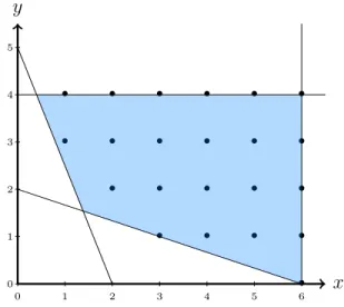
x y 0 1 2 3 4 5 6 7 0 1 2 3 4 5 5x + 7y = 35 5x + 7y = 25 5x + 7y ≈17 .7
Figure 3.1: Feasible region for constraintsy≤4, x≤6, 5x+ 2y≥10, andx+ 3y≥6.
Definition 6 The feasible region of an LP is the set of all points that satisfies its con-straints. In other words, it is the set of all solutions for an LP.
Example 6 In Figure 3.1 the shaded area represents the feasible region for a linear pro-gram with linear inequality constraints constraints y ≤ 4, x ≤ 6, 5x + 2y ≥ 10 and
x+ 3y≥6.
Definition 7 A solution for an LP that minimizes the objective function value over all solutions of the LP is an optimal solution.
If the feasible region for an LP is empty, then there are no assignments for variables that satisfy the linear constraints of the LP. In this case we say that the linear program is infeasible. To give more intuition on linear programming let us consider the following LP instance.
Example 7 Consider the following LP.
Minimize 5x+ 7y subject to 5x+ 2y≥10 x+ 3y ≥6 x≤6 y≤4 x, y ≥0.
16
Now in the Figure 3.1 a dashed line represents a contour line, i.e., all points that have the same objective function value. Once we have decreased the value so that the line intersects with the last extreme point, i.e., a corner of the feasible region, we have found an optimal solution. For this linear program the optimal solution sets x = 18/13 and y = 20/13
resulting in an objective function value of 230/13≈17.7
Finding a solution to linear program can be done in polynomial time [61]. Encoding NP-hard problems compactly into LP instances cannot be done unless P = NP.
3.2
Integer Linear Programming Definitions
Linear programming is a special case of integer linear programming, or ILP [93, 85, 27, 25] for short. Similarly to a linear program, an integer linear program is an optimization problem, where the goal is to minimize a linear objective function consisting ofn variables x1, . . . , xn while being subject to linear inequality constraints. The difference is that the
problem also has integrality constraints meaning that some of the variables are forced to be integers. More formally any ILP can be expressed in the following form.
Minimize: Xn j=1 cj·xj subject to Xn j=1 aij ·xj ◦bi, i= 1, . . . , m, xj ∈Z where ◦ ∈ {<,≤, >,≥,=}.
As the integrality constraints in the ILP instances considered in this thesis are constrained to be binary values zero and one, we can consider special case for the ILP known as 0-1 ILP or binary ILP.
Finding a solution for this binary ILP problem is known to be NP-complete [81] as SAT can be reduced to it.
To give an example on how to model problems in ILP, let us consider the graph coloring problem and the vertex cover problem.
Example 8 Consider again the graph coloring problem described in Example 5. Let k be the number of vertices. The problem can be modeled as an linear program as follows.
Minimize
k
X
i=1
ci for each color 1≤i≤k ,
subject to
k
X
i=1
xv,i >0, for each vertex v ∈V ,
xv,i+xu,i ≤1, for each edge (v, u)∈E and 1≤i≤k ,
xv,i−ci ≤0, for each vertex v ∈V and 1≤i≤k ,
xv,i, ci ∈ {0,1}, for all v ∈V and 1≤i≤k.
The objective function corresponds to the sum of all used colors. The first constraint corresponds to forcing a single color assignment on each vertex. The second constraint corresponds to forcing adjacent vertices to not have the same assigned color. The third constraint forces assinging ci to one if the corresponding color has been assigned to some
vertex. An optimal solution to this integral linear program corresponds to an optimal solution for graph coloring problem.
Example 9 In the vertex cover problem, we are given an undirected graph G = (V, E), for which we must find a minimum set of vertices, such that each edge of the graph is incident to at least one of the vertices in the vertex cover. This problem can be formulated as an ILP as follows.
Minimize X
v∈V
xv, for all v ∈V
subject to xu +xv ≥1, for all edges (u, v)∈E
xv ∈ {0,1}, for all v ∈V
Herexv = 1corresponds to a vertex being picked for the vertex cover. With this formulation
we can find an optimal solution to an instance of the minimum vertex cover problem.
3.3
LP Relaxation and Approximations
While ILP is NP-hard, removing the integrality constraints creates a related LP problem that can be solved in polynomial time. This is called an LP relaxation [89, 53, 52, 67, 68] of the ILP. Removing the integrality constraint means that we relax the constraintx∈Z
18
to a constraint x∈R. For a 0-1 ILP we relax the binary constraintx∈ {0,1}to a linear constraint 0 ≤x≤1. Solution for the LP relaxation can be used as a lower bound on an
optimal solution for the original ILP instance.
Example 10 Consider the following ILP.
Minimize 5x+ 7y subject to 5x+ 2y ≥10, x+ 3y≥6, x≤6, y≤4, y, x∈N.
The LP relaxation of this ILP is obtained by relaxing the last constraint y, x ∈ N to y, x≥0. This results in the following LP.
Minimize 5x+ 7y, subject to 5x+ 2y ≥10, x+ 3y≥6, x≤6, y≤4, y, x≥0.
In Figure 3.2 we can see the feasible points for the ILP instance and feasible region for the LP relaxation is the shaded area.
Solutions for the LP relaxation can be solutions for the original ILP instance but they do not have to be. The solution might assign non-integer values for variables. For example, if the goal was to maximize the sum x+y and the only linear constraint is x+y < 2, an optimal solution assigns x or y a fractional value. However, if solving the relaxed ILP instance assigns only integer values to the variables then it is also a solution for the original ILP problem. In the former case, where the solution to LP relaxation is not a
x y 0 1 2 3 4 5 6 0 1 2 3 4 5 • • • • • • • • • • • • • • • • • • • • • •
Figure 3.2: Feasible points for an ILP instance and feasible region for its LP relaxation. solution original ILP instance, in some cases we can still use the solution for LP relaxation instance to form a solution for the ILP instance. This can be done with rounding, i.e., by rounding the non-integer values in the solution for LP relaxation to be integers. This then gives us an approximation of the optimal solution for the ILP instance. This can create an approximation algorithm for the original problem.
Definition 8 A c-approximation algorithm gives a solution that is a factor ofcaway from the optimal solution for minimization problems. More formally, given an optimal solution
OP T, a c-approximation algorithm results in a solution S for which S ≤c·OP T.
Rounding approaches are problem-specific. This means that while certain rounding pro-cedure can result in solutions for one problem, for other problems it might not. To give intuition on how LP relaxation and rounding works, let us consider the previously men-tioned vertex cover example.
Example 11 The LP relaxation of the ILP formulation of the vertex cover problem in Example 9 results in the following linear program.
Minimize X
v∈V
cv·xv
subject to xu+xv ≥1 for all {u, v} ∈E,
20
Now with this relaxation, the variables can be assigned to values between zero and one. To round the given solution to the relaxed instance we can apply a very simple rounding strategy of using 1/2 as a threshold for rounding. All variables with value below this threshold will be rounded to zero and variables with value equal or above this threshold will be rounded to one. Now since each edge (v, u) ∈ E has a corresponding constraint
xv +xu ≥1, both of the vertices must have a value of at least 1/2, meaning the rounding
will set at least one of the variables to one. This corresponds to picking at least one vertex for each edge in the vertex cover problem. From this it follows that all solutions obtained from this rounding are solutions for the original vertex cover problem. In the worst case where every variable has been assigned a value of1/2this rounding will result in a solution that has two times the number of vertices in vertex cover compared to an optimal solution. Therefore this rounding strategy gives us a 2-approximation algorithm for the vertex cover problem [102].
With some graphs this approach can result in an optimal solution but not always. Consider the two following examples.
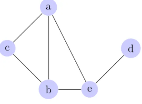
Example 12 Let G = (V, E) be a graph, where V ={a, b, c, d, e} and E ={(a, b),(a, c), (a, e),(b, c),(b, e),(e, d)}. Figure 3.3 illustrates this graph. With this graph, the LP relax-ation gives each vertex the following values a = 9/10, b = 3/5, c = 2/5, d = 9/10 and
e = 2/5. Now if we use the previously mentioned rounding that uses threshold of 1/2 we obtain an assignment, where a = 1, b = 1, c= 0, d = 1 and e = 0 giving us a solution with the objective function value of three. This is also an optimal solution to the problem instance in question.
a
b
c d
e
Figure 3.3: Undirected graph G
As we can see this simple rounding scheme gave us an optimal solution for a specific vertex cover instance. Now let us consider an instance where the LP relaxation and rounding does not result in an optimal solution.
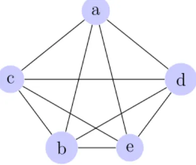
Example 13 Let G0 = (V, E) be a graph, where V = {a, b, c, d, e} and there is an edge between each node (graph is a clique). Figure 3.4 illustrates this graph. Now for each vertex the LP relaxation assigns for each vertex v ∈ V a value of 1/2. Now if we use the same rounding strategy as before, we obtain a solution that that assigns a =b= c=d=e = 1
which has the objective function value of five. However, an optimal solution to this problem has four vertices in vertex cover, meaning that the solution given by the LP relaxation rounding is not optimal.
a
b
c d
e
Figure 3.4: Undirected graph G’
From Examples 12 and 13 we can see that the LP relaxation rounding can result in an optimal solution to the problem in question but cannot guarantee it. Depending on the problem there are other rounding strategies that can result in better quality solutions. For example we could use randomized rounding where the rounding is decided by probability of the assigned value, i.e., a variable xi is rounded to one with the probability of xi and
to zero with the probability of 1−xi. However, depending on the problem we are trying
to solve, a rounding method like this could lead to solutions that do not satisfy the linear constraints of the problem. In the vertex cover problem, for example, nothing guarantees that for each edge (v, u) ∈ E either xv or xu would be assigned a value of one which
corresponds to neither of them being guaranteed to be in the vertex cover.
3.4
ILP Solving
Central approaches for solving ILP problems include branch and bound [1, 99], the cutting plane method [43, 44] and the branch and cut method [87, 16]. All of these methods use the LP relaxation as a part of the solving process.
Branch and bound solves ILP problems by first solving the LP relaxation. Then the algorithm checks if all variables are integers. If so an optimal solution is found. Otherwise
22
the algorithm branches, i.e., bounds the non-integer variables with lower bound on the other branch and upper bound on the other branch. For example ifx= 7/3 then branching would be done by adding new bound x≤ 2 on the other branch and bound x≥ 3 to the other branch. This is then repeated until an optimal solution is found or the ILP is found to be infeasible.
The general idea of the cutting plane method is that the LP relaxation for the ILP instance is first solved. Once we have the solution for LP instance we check if the variables are integer. If yes then we found an optimal solution and the algorithm terminates. If not we add a new constraint to the LP relaxation that essentially cuts the section of the feasible region where an optimal solution for LP was found but does not have the solution for the ILP instance.
Branch and cut can be considered a combination of branch and bound and cutting plane methods. Similarly to branch and bound and cutting planes method, branch and cut first solves the LP relaxation of the ILP instance. The algorithm then proceeds similarly to branch and bound but for each node cutting planes are searched. This helps the algorithm to have more tighter bounds on the non-integer values than regular branch and bound approach.
3.5
LP Solving
Two notable types of algorithms for solving LP instances are simplex [26, 58, 33] and inte-rior point [59, 79, 86] methods. Depending on the problem being solved one method might work better than the other but for the most part both of these methods are competitive with each other [51].
The simplex method
The simplex algorithm (or method) is a classic optimization method for solving linear programs. The simplex method uses the fact that an optimal solution is found in one of the extreme points of the feasible region formed by the linear constraints of the LP. The algorithm starts from one extreme point and then checks if it is an optimal solution. If not it moves along the edge of the feasible region to a next extreme point and again checks the optimality of the found solution. Basically the simplex algorithm traverses along the edges of the feasible region of a linear program finding increasingly better solutions until
it finds an optimal solution. This algorithm can take exponential time in the worst case [62]. However, in most real-life applications the simplex method runs in polynomial time [95].
Interior-point method
Another central method to solve linear program is the interior-point method . Where as the simplex algorithm traversed along the edges of the feasible region the interior point method traverses through the interior of feasible region. At each iteration the algorithm checks if it has converged to one of the feasible regions extreme points. If so the algorithm stops and an optimal solution is found. Otherwise the algorithm computes a search direction, moves and again checks for convergence. The algorithm keeps doing this until it finds an optimal solution. This method has been shown to run in polynomial time [59]. Linear programs were shown to be polynomial time solvable before with ellipsoid method [61] but was too slow for practical use. Interior-point method had better worst case complexity and created more interest in developing better algorithms for solving LP problems [96, 104].
4 LP Relaxations for Incomplete
MaxSAT Solving
We explore using LP relaxations and rounding to solve MaxSAT instances. As mentioned in prior chapters ILP can be used to solve MaxSAT instances. In this chapter we first go over in Section 4.1 how MaxSAT instances are encoded as ILP. In Section 4.2 we go over the LP relaxation of the ILP and present rounding procedures which we will empirically evaluate. Finally in Section 4.3 we discuss how these rounding procedures were implemented.
4.1
Encoding MaxSAT to ILP
To solve MaxSAT via ILP we use a standard encoding of MaxSAT to ILP presented in the literature [6, 41, 70, 74]. Given a MaxSAT formula F we encode it to an ILP as follows. For a clause Ci ∈ F, let Ci+ be the set of indices of the positive literals appearing in a
clause Ci and Ci− the set of indices of the negative literals appearing in a clause Ci.
Definition 9 Given a partial MaxSAT instance F = (Fh, Fs, w), let ILP(F) be the
fol-lowing ILP.
Minimize X
Ci∈Fs
w(Ci)·bi, where w(Ci) is the weight of clause Ci
subject to X j∈Ci+ xj + X j∈Ci− (1−xj)>0, for each Ci ∈Fh X j∈Ci+ xj + X j∈Ci− (1−xj) +bi >0, for each Ci ∈Fs x, y, bi ∈ {0,1}.
In this formulation, for each soft clause Ci ∈ F we introduce a new binary relaxation
variablebi. The objective function takes a sum over all the weights and the corresponding
where bi = 1, the cost of the objective function increases by the associated weight. For
each clause C ∈F a linear inequality constraint is formed by taking the sum P
j∈Ci+xj +
P
j∈Ci−(1−xj) over all the literals in a clause. In order for this sum to correspond to a
satisfying truth assignment, the sum needs to be greater than zero. For the soft clauses a corresponding relaxation variable bi is added to the sum. Now a solution for this ILP
must assign eitherxj = 1 forj ∈Ci+, xj = 0 forj ∈Ci− in each clauseC ∈F orbi = 1 for
each soft clause C ∈ Fs. Therefore, any solution obtained for ILP(F) will be a solution
for the MaxSAT instanceF. Furthermore, any optimal solution found for the ILP(F) will be an optimal solution forF. Let us consider the following example.
Example 14 Consider the MaxSAT instanceF ={(x∨y,3),(¬x∨y,4),(x∨¬y,2),(¬x∨
¬y,10)}. Now ILP(F) is Minimize 3·b1+ 4·b2+ 2·b3+ 10·b4 subject to x+y+b1 >0, −x+y+b2 >−1, x−y+b3 >−1, −x−y+b4 >−2, x, y, bi ∈ {0,1}.
An optimal solution for this integer linear program assigns x = 0, y = 1 and b3 = 1
resulting in the cost of two.
Solving MaxSAT instances encoded this way to ILP using ILP solvers has been shown to be competitive in some problem domains [6, 28].
4.2
Rounding LP Relaxations for MaxSAT
Using LP relaxations and rounding to obtain a solution for NP-hard optimization problems is well studied [23, 19, 2, 97, 49, 15]. As discussed in the previous chapter, ILP has been found to be a rather efficient approach for some MaxSAT instances [6, 28]. Removing the integrality constraints from the ILP formulation and rounding the solution for the LP relaxation speeds up solving MaxSAT instances at the cost of losing (guaranteed)
26
optimality of the found solution. To show that rounding a solution for LP relaxation does not guarantee optimality, let us consider the following example.
Example 15 Let F be the same MaxSAT instance as in Example 14. Now the LP relax-ation of ILP(F) is as follows.
Minimize 3·b1+ 4·b2+ 2·b3+ 10·b4 subject to x+y+b1 >0, −x+y+b2 >−1, x−y+b3 >−1, −x−y+b4 >−2, x, y, bi ∈[0,1].
An optimal solution for this LP assigns x =y= 1/2 and bi = 0 for 1≤ i≤4. Rounding
this solution to integers with a rounding strategy that sets x = 1 if 1/2 ≤ x and x = 0
otherwise, we obtain a solution that assigns x =y = 1. The solution obtained using this rounding satisfies the first three constraints. The constraint −x−y +b4 > −2 is not
satisfied meaning that we must assign b4 = 1. Assigning b4 = 1 incurs a cost of 10. This
is not an optimal solution since a solution that assigns x= 0, y= 1 and b3 = 1 has a cost
of two.
If we only consider non-partial MaxSAT instances and only apply rounding to
non-relaxation variables, we can always assign values to non-relaxation variables in a way that guarantees the obtained assignment to be a solution. This is due to the fact that there are no clauses that must be satisfied in order for a truth assignment to be a solution. Rounding should hence be only applied on variables corresponding literals of the MaxSAT instance.
Rounding relaxation variables can create too tight bounds creating assignments that are not solutions for the ILP, which is why in this work we do not round relaxation variables. While relaxation variables could be rounded in theory, it requires more care and is left as future work. Consider the following example.
Example 16 Let F be an unweighted non-partial MaxSAT instance. Assume that F has a clause C = (x∨y). ILP(F) contains the linear constraintx+y+bC >0. Assume that
solving the LP relaxation of the ILP(F)we would obtain an assignmentx=y=bC = 5/12.
This would still be a solution for the LP relaxation as the sumx+y+bC = 3·5/12>1>0.
The rounding procedure that would round all variables below 1/2 to zero would result in a solution that would not satisfy the linear constraint x+y+bC > 0. Therefore, the
assignment resulting from this rounding would not be a solution for the ILP.
The rounding methods considered in this thesis can be split into two categories: threshold rounding and iterative rounding. Threshold rounding methods solve the LP relaxation once and then apply rounding to all non-relaxation variables. Iterative rounding methods solve the LP relaxation, round at least one non-relaxation variable to either zero or one, update LP relaxation by fixing said variable to what it was rounded, i.e., add constraint xi = 1 or xi = 0 to the LP relaxation, and solve the updated LP relaxation. This
is iteratively done until all non-relaxation variables have been fixed. The most obvious difference between these two types of rounding methods is that the threshold rounding methods are faster than the iterative rounding methods. This is due to threshold methods having to solve the LP relaxation only once. While iterative methods are slower, at each iteration a new solution obtained for the updated LP relaxation can guide the approach toward solutions of better quality.
4.2.1
Threshold Rounding
The first set of rounding methods we consider are threshold rounding methods. Algorithm 1 outlines a general threshold rounding algorithm. Given a MaxSAT instance F the algorithm first obtains the LP relaxation of ILP(F) on line 1. Then on line 3 it calls a LP solver to solve the LP relaxation and saves the obtained solution into sol. Finally all
non-relaxation variables are rounded by a rounding procedure on lines 4-6. In this thesis
Algorithm 1: General threshold rounding input:MaxSAT instance F
1 L0 = LP relaxation ofILP(F) 2 literals = a set of all variables in F 3 sol=solve(L0)
4 foreach x∈literals do 5 rounding procedure 6 end
28
we consider three threshold rounding schemes which we will refer to as Simple,Random and CF.
Algorithm 2 outlines Simple, the first rounding approach we consider. This algorithm rounds a variable x to one ifv ≥1/2 and to zero otherwise, where v is the value assigned to x in the solution for the LP relaxation. More specifically, it first creates a variable v on line 1 that gets a value that was assigned for the variable x in solution sol for the LP
relaxation. Then on line 2 it checks whether the value v is greater than or equal to 1/2. If it is greater or equal, x is rounded to one and to zero otherwise.
Algorithm 2: Simple rounding (Simple) input: Variable x and solutionsol
1 v = value assigned to x by solution sol 2 if v ≥1/2 then x= 1
3 else x= 0
Algorithm 3 outlines the second threshold rounding approach Random. This algorithm rounds a variable to one with the probability of v, where v is the value assigned to a variable x in the LP solution sol and to zero with the probability of 1−v. On line 2 the
algorithm computes for each variable x a random number r between zero and one. If the number r is less than the value assigned to variable x in the sol, we set the variable to
one and to zero otherwise. For example, if we have a solution to the LP relaxation where x = 2/3 and y = 1/3, x would be more likely set to one and y to zero. However, there is a possibility that both of these variables would be rounded to the opposite of what they were closest to, i.e., if assigned value was closer to one it would be rounded to zero and vice versa. Rounding variables this way has been shown to result in a (1−1
e)−approximation
algorithm [41].
Algorithm 3: Random rounding (Random) input: Variable x and solutionsol
1 v = value assigned to x by solution sol 2 r = random number between 0 and 1 3 if r≤v then x= 1
4 else x= 0
Algorithm 4 outlines the final considered threshold rounding method CF. CF takes the previously mentioned Random algorithm and combines it with a (1/2)-approximation
Algorithm 4: Coin-flip rounding (CF) input:Variable x and solution sol
1 r1 = random number between 0 and 1 2 if 1/2≤r then
3 Random(x,sol) 4 else
5 r2 = random number between 0 and 1 6 if 1/2≤r2 then x= 1
7 else x= 0 8 end
algorithm [106, 55], where each variable is set to one with probability of 1/2 and to zero otherwise. For each variablexthe algorithm first picks a random numberr1 between zero and one at line 1. If the value of r1 is greater or equal to 1/2, then at line 5 CF calls the rounding procedureRandom. Otherwise, the algorithm picks a new random number
r2 between zero and one. If the value ofr2 is greater or equal to 1/2, then the algorithm
assigns x = 1 and x = 0 otherwise. This rounding approach has been shown to be a 3/4-approximation algorithm [41].
4.2.2
Iterative Rounding
The other set of rounding approaches we focus on are the so-called iterative rounding methods. Given a MaxSAT instance F, algorithms that are iterative work by solving the LP relaxation of the ILP(F), then fixing at least one variable to one or zero and
then solving the instance again with the fixed variables. Compared to threshold methods,
Algorithm 5: General iterative rounding input:MaxSAT instance F
1 L0 = LP relaxation ofILP(F) 2 literals = a set of all literals in F 3 while length(literals)>0 do 4 sol=solve(L0)
5 rounding procedure 6 end
30
iterative methods tighten the feasible region at each iteration. This way the algorithm can be, in theory, guided towards a better quality solution after fixing a variable. On the other hand, iterative rounding can be more time-consuming as the LP relaxation must be solved multiple times before we obtain a solution. Algorithm 5 outlines the structure of the general iterative rounding algorithm. Lines 1-2 are the same as in Algorithm 1. At line 4 the algorithm starts a while loop that will terminate once the set literals is empty. At
each iteration each rounding procedure will remove the fixed variables from this set. First step at each iteration is to solve the LP relaxation. Then the algorithm calls a rounding procedure at line 6. In this thesis we consider the following iterative rounding schemes: Iter, IterBatch, IterRandd and BoRB.
Algorithm 6: (Simple) Iterative rounding (Iter) input: Set literals, solution sol and LP relaxation L0
1 best =x∈literals that maximizes|1/2−value of x insol | 2 v = value assigned to variable best in solution sol
3 if v ≥1/2 then add var(best) = 1 to L0 4 else add var(best) = 0 toL0
5 remove var(best) from literals
Algorithm 6 outlines the first iterative rounding methodIter, where we round one variable to either one or zero. After the LP relaxation has been solved the algorithm finds the variable x that has been assigned value farthest away from 1/2 in the sol at line 1, i.e.,
the variable that maximizes|1/2−x|. Once such a variable is found the algorithm rounds the variable to which value it is closer to, zero or one. At line 5 the algorithm removes the now fixed variable from the literals.
Algorithm 7: Iterative batch rounding (IterBatch)
input: Set literals, integer k, solution sol and LP relaxation L0
1 batch = pick k number of variables for which |1/2−value of xin sol | is maximized 2 foreach x∈batch do
3 if v ≥1/2 then add var(x) = 1 toL0 4 else add var(x) = 0 toL0
5 remove var(x) from literals 6 end
this approach. Overall this algorithm works similarly to algorithm outlined in Algorithm 6. However, instead of fixing only one variable, a batch of k variables are fixed at each iteration. At line 1 IterBatch takes a k number of variables that have been assigned a value farthest away from 1/2 in the sol. The LP relaxation is then updated by fixing
all variables in the batch to the value obtained by rounding each variable to which value they are closest to, zero or one. Then the variables in the batch are all removed from the setliterals. The idea behind this approach is to keep the iterative approach but speed up
the solving process by fixing more variables at each iteration which lowers the number of required solver calls.
Algorithm 8: Iterative randomized rounding (IterRand) input:Set literals, integer k, solution sol and LP relaxation L0
1 batch = pick k number of variables for which |1/2−value of x insol | is maximized 2 x= uniformly at random chosen variable from batch
3 if v ≥1/2then add var(x) = 1 to L0 4 else add var(x) = 0 toL0
5 remove var(x) from literals
Iterative Randomized, or IterRand, rounding outlined by Algorithm 8 initially works similarly to batching as it takes a batch of variables. The difference between these two is that the IterRand at line 2 picks one variable from batch uniformly at random. The LP relaxation is then updated by fixing this randomly chosen variable to value obtained by rounding it to which value it is closer to, zero or one. Then the variable is removed from the setliterals. Randomizing the variable selection can direct the rounding algorithm
away from getting stuck in bad local optima.
Algorithm 9: Best of randomized batch rounding (BoRB) input:Set literals, integer k, solution sol and LP relaxation L0
1 randomBatch = pick k number of variables uniformly at random from literals 2 x= x∈randomBatchthat maximizes |1/2−value of xin sol |
3 if v ≥1/2then add var(x) = 1 to L0 4 else add var(x) = 0 toL0
5 remove var(x) from literals
Best of randomized batch, or BoRB, rounding outlined in Algorithm 9 employs a more aggressive randomization. At line 1 instead of picking batch of best variables as before,
32
the algorithm picks uniformly at random k variables. From this randomized batch a variable that has been assigned a value that is farthest away from 1/2. The LP relaxation is then updated by fixing the variable to value obtained by rounding the variable to which value it is closer to, zero or one. Then the variable is removed from the set literals.
Randomization inIterRandhappened among the best candidates which might still leave us stuck in a bad local optima. In BoRB the randomization happens during selection of the candidate variables To balance the aggressive randomization BoRB picks a best
candidate for rounding.
4.3
Implementation
The rounding approaches Simple, Random, CF, Iter, IterBatch, IterRand and BoRB were all implemented on top of the SCIP [38, 39] framework. SCIP is a frame-work for constraint integer programming that is developed at Konrad-Zuse-Zentrum f¨ur Informationstechnik Berlin. The underlying LP solver in SCIP is SoPlex [36, 37] which implements the simplex algorithm.
For each rounding approach, a given MaxSAT instance F is first transformed into the LP relaxation of ILP(F) with a Python script and then passed to the rounding
proce-dure. A simple bash script handles passing these files to rounding scripts and usesulimit
-t <number-of-seconds> command to make sure rounding terminates in case of
time-out. We opted on implementing rounding scripts by using Python 2.7 and therefore used PySCIPOpt which is a Python interface for SCIP.
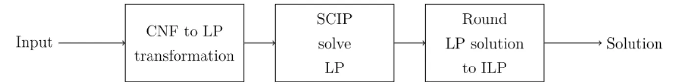
Input CNF to LP transformation SCIP solve LP Round LP solution to ILP Solution
Figure 4.1: Flow of threshold script design
Scripts for Simple,Random andCFfirst read the problem into memory and calls SCIP to solve the LP instance. Once the instance has been solved by SCIP, a simple for loop fixes all variables using a corresponding rounding procedure. After rounding the cost of the solution is computed. The flow of these three scripts is illustrated by Figure 4.1. Scripts for Iter, IterBatch, IterRand and BoRB were implemented by a simple while loop that terminates once all variables have been fixed. At each loop SCIP is asked
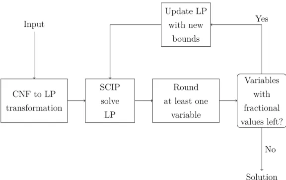
to solve the LP relaxation of the original instance with the fixed variables. After there are no variables to fix the cost of the solution is computed. Figure 4.2 illustrates the flow.
Input CNF to LP transformation SCIP solve LP Round at least one variable Variables with fractional values left? Solution Update LP with new bounds Yes No
Figure 4.2: Flow of iterative script design
As a further heuristic in iterative methods we fixed all variables that were assigned to zero or to one in the solution for LP relaxation obtained by