Exploiting Diversity for Optimizing Margin
Distribution in Ensemble Learning
Qinghua Hua, Leijun Lia, Xiangqian Wua, Gerald Schaeferb and Daren Yuc
a
Biometric Computing Research Centre, School of Computer Science and Technology, Harbin Institute of Technology, Harbin 150001, China
b
Department of Computer Science, Loughborough University, U.K. c
School of Energy Science and Engineering, Harbin Institute of Technology, Harbin 150001, China
Abstract
Margin distribution is acknowledged as an important factor for improving the generalization performance of classifiers. In this paper, we propose a novel ensemble learning algorithm named Double Rotation Margin Forest (DRMF), that aims to improve the margin distribution of the combined system over the training set. We utilise random rotation to produce diverse base classifiers, and optimize the margin distribution to exploit the diversity for producing an optimal ensemble. We demonstrate that diverse base classifiers are beneficial in deriving large-margin ensembles, and that therefore our proposed technique will lead to good generalization performance. We examine our method on an extensive set of benchmark classification tasks. The experimental results confirm that DRMF outperforms other classical ensemble algorithms such as Bagging, AdaBoostM1 and Rotation Forest. The success of DRMF is explained from the viewpoints of margin distribution and diversity.
Keywords: Ensemble learning, margin distribution, diversity, fusion strategy, rotation
1. Introduction
Ensemble learning has been an active research area in pattern recognition and machine learning domains for more than twenty years [1, 29, 38, 45, 59]. Ensemble learning, also referred to as multiple classifier systems, committees of learners, decision forest or consensus theory, is based on the idea of training a set of base classifiers or regressors for a given learning task and combining their outputs through a fusion strategy.
A significant amount of works have been focused on designing effective en-semble classifiers [15, 20, 25, 39]. However, an exact explanation of the success
Email address: [email protected], [email protected], [email protected], [email protected], [email protected](Qinghua Hua
, Leijun Lia , Xiangqian Wua , Gerald Schaeferb and Daren Yuc )
of ensemble strategies is still an open problem. Some researchers explored how an ensemble’s effectiveness is related to the large margin principle, which is regarded as an important factor for improving classification [42, 51]. In this paper, we propose a novel ensemble learning algorithm named Double Rotation Margin Forest (DRMF), which is designed to improve the margin distribution of ensembles by enhancing the diversity of base classifiers and exploiting this diversity using an optimization technique.
In general, there are two well-accepted viewpoints – diversity and margin – to explain the success of ensemble learning. Roughly speaking, the margin of a sample is its distance from the decision boundary and thus reflects the confidence of the classification. The margin distribution is acknowledged as an important factor for improving the generalization performance of classifiers [2, 6, 11, 43, 49]. In [43], Shawe-Tayloret al. gave an upper bound of generalization error in terms of the margin, while in [6] a similar bound was derived for neural networks with small weights. The large margin principle has been employed to design classification algorithms in [8, 14, 21, 26, 50].
The performance of ensemble learning methods, especially boosting, has been attributed to the improvement of the margin distribution of the training set [42, 51]. In AdaBoost, each new base classifier is trained by taking into account the performance of the previous base classifiers. Training samples that are misclassified by the current base classifiers play a more important role in training the subsequent one. The success of Adaboost can thus be explained from the margin distribution, where the optimization objective is to minimize a margin distribution based exponential loss function. In [42], an upper bound of the generalization error was derived in terms of the margins of the training samples, and it was shown that the generalization performance was determined by the margin distribution, the number of training samples and the number of base classifiers. The efficacy of AdaBoost thus lies in its ability of effectively improving the margin distribution. In [51], Wang et al. showed that a larger Equilibrium margin (Emargin) and a smaller Emargin error can reduce the generalization error, and demonstrated that AdaBoost can produce a larger Emargin and a smaller Emargin error.
It is acknowledged that the diversity among the members of an ensemble is crucial for performance improvement. Intuitively, no improvement can be achieved when a set of identical classifiers are combined. Diversity thus allows different classifiers to offer complementary information for classification, which in turn can lead to better performance [28]. A number of techniques have been proposed to introduce diversity. In general, we can divide these into two cat-egories: classifier perturbation and sample perturbation approaches. Classifier perturbation refers to the adoption of instability of learning algorithms [10, 36] such as decision trees and neural networks. Since they are sensitive to initial-ization, trained predictors may converge to different local minima if started from different initializations, and diversity can thus be generated from trained classifiers. Sample perturbation techniques train classifiers on different sample subsets or feature subsets, and include bagging, boosting, random subspaces and similar approaches [4, 7, 17, 41].
Since both diversity and margin are argued to explain the success of ensemble learning, it appears natural to question whether there is a connection between the two. Tang et al. [46] proved that maximizing the diversity among base classifiers is equivalent to optimizing the margin of an ensemble on the training samples if the average classification accuracy is constant and maximal diversity is achievable. Consequently, increasing the diversity among base classifiers is an effective method to improve the margin of ensembles. Our work is motivated by this conclusion, and our aim is to improve the margin distribution of ensembles. In our proposed approach, we enhance the diversity of base classifiers by perturbing the samples using double random rotation. This idea is inspired by the PCA rotation proposed in the Rotation Forest algorithm [39]. In Rotation Forest, a candidate feature set is randomly split into K subsets and Princi-pal Component Analysis (PCA) is conducted on each subset to create diverse training samples. Diversity is thus promoted through the random feature splits for different base classifiers. In our work, the feature sets are also randomly split into K subsets. In order to introduce further diversity between the base classifiers, we apply PCA and Locality Sensitive Discriminant Analysis (LSDA). In particular, we first perform unsupervised rotation with PCA, and then em-ploy supervised large-margin rotation with LSDA. LSDA [12], as a supervised method, is able to derive a projection which maximizes the margin between data points from different classes. Our experimental results show that the ap-plied Double Rotation can consistently enhance the diversity in a set of base classifiers.
We further exploit the diversity and improve the margin distribution with an optimal fusion strategy. In principle, there are two kinds of fusion strategies. One approach is to combine all available classifiers, e.g., in simple (plurality) voting (SV) [28] or through linear or non-linear combination rules [5, 9, 19, 48]. The other method is to derive selective ensembles, or pruned ensembles such as LP-Adaboost [23] or genetic algorithm (GA)-based approaches [53], which only select a fraction of the base classifiers for decision making and discard the others. Clearly, the key problem here is how to find an optimal subset of base classifiers [32]. In the GASEN approach [55], neural networks are selected based on evolved weights to constitute the ensemble. In [54], the subset selection problem is formulated as a quadratic integer programming problem, and semi-definite programming is adopted to select the base classifiers. Both GASEN and semi-definite programming are global optimization methods and thus their com-putational complexity is rather high. Suboptimal ensemble pruning methods were proposed to overcome this drawback, including reduce-error pruning [31], margin distance minimization (MDM) [33], orientation ordering [34], boosting-based ordering [35], and expectation propagation [13]. In practice, users would prefer sparse ensembles since computational resources are often limited [57]. In this paper, we introduce a technique to improve the margin distribution by minimizing the margin induced classification loss. In our pruned ensembles, the weights of base classifiers are trained withL1regularized squared loss [56]. The base classifiers are then sorted according to their weights, and those with large weights are selected in the final ensemble.
Our presented work comprises three major contributions. First, since di-versity is considered to be an important factor which affects the classification margin, Double Rotation is proposed to enhance the diversity among base clas-sifiers. Second, we present a new pruned fusion method based on the Lasso technique for generating ensembles with optimal margin and sparse weight vec-tors, where the weights are learned through minimization of the regularized squared loss function. Third, we present an extensive set of experiments to evaluate the effectiveness and explain the rationality of the proposed algorithm. We convincingly show that it can improve the margin distribution to a great extent and lead to powerful ensembles.
The remainder of the paper is organized as follows. Related work is in-troduced in Section 2. Section 3 describes our proposed algorithm, while an analysis in terms of parameter sensitivity and robustness is presented in Sec-tion 4. SecSec-tion 5 presents the experimental results and explores the raSec-tionality of DRMF. Finally, Section 6 offers conclusions and future work.
2. Related Work
Assume that xi = [xi1,· · · , xin]T is a sample represented by a set F of n features and every sample is generated independently at random according to some fixed but unknown distributionD. LetX be anN×nmatrix containing
the training set andY = [y1,· · ·, yN]T be anN-dimensional vector containing the class labels for the data, where yi is a class label of xi from the set of the class labels {ω1,· · · , ωc}. Let {C1,· · · ,CL} be the set of base classifiers in an ensemble. In this paper, our aim is to obtain an ensemble system with small generalization error via optimizing the margin distribution. Here, the generalization error of a classifier Cj is the probability of Cj(x) 6= y when an example (x, y) is chosen at random according to the distributionDand denoted
as PD[Cj(x) 6=y]. The margin distribution is a function of θ which gives the fraction of samples whose margin is smaller thanθ. A good margin distribution means that most examples have large margins.
Definition 1. Given xi ∈X, hij(j = 1,2· · ·, L) is the output of xi from Cj.
We define
dij =
1, ifyi=hij
−1, ifyi6=hij , (1)
where yi is the real class label of xi.
From this definition, we know thatdij = 1 ifxi is correctly classified byCj; otherwisedij =−1.
Definition 2. [42] Givenxi∈X, the margin ofxi in terms of the ensemble is
defined as m(xi) = L X j=1 wjdij, (2)
In [42, 51], it is shown that a small generalization error for a voting classifier can be obtained by a good margin distribution on the training set. Obviously, the performances of the base classifiers have a significant effect on the margin of xi. At the same time, the diversity among base classifiers is another key factor. In [46], the underlying relationship between diversity and margin was analyzed.
Theorem 1. [46] Let Θbe the average classification accuracy of the base clas-sifiers. If Θis regarded as a constant and if maximum diversity is achievable, maximization of the diversity among base classifiers is equivalent to maximiza-tion of the minimal margin of the ensemble on the training samples.
It should be noted that our aim is not to maximize the minimal margin of the ensemble, but to optimize the margin distribution. We use a disagreement measure [30] to measure the diversity of the base classifiers in our approach. The diversity between classifiers Cj andCk is thus computed as
Disjk=
N01+N10
N11+N10+N01+N00, (3)
whereN00denotes the number of samples misclassified by both classifiers,N11 is the number of samples correctly classified by both, N10denotes the number of samples which were correctly classified byCj but misclassified byCk, andN01 denotes the number of samples misclassified byCj but correctly classified byCk. For multiple base classifiers, the overall diversity is computed as the average diversity of classifier pairs.
In [39], Rodr´ıguez and Kuncheva designed a method to generate ensembles based on feature transformation. The diversity of base classifiers is promoted by random splits of the feature set into different subsets. The original feature space is split intoK subspaces (the subsets may be disjoint or may intersect). Then, PCA is applied to linearly rotate the subspaces along the “rotation” matrix. Diversity is obtained by random splits of the feature set.
Caiet al. [12] proposed a supervised algorithm for feature transformation, which can find a projection that maximizes the margin between different classes. For xi ∈X, denote by Υ(xi) ={xi1,· · ·, xei} the set of itse nearest neighbors and byyi the class label ofxi. We define
Υs(xi) ={xji|y j i =yi,1≤j≤e}, (4) and Υb(xi) ={xji|y j i 6=yi,1≤j ≤e}, (5)
so that Υs(xi) contains the neighbors which share the same label withxi, while Υb(xi) is the set of the neighbors which belong to the other classes.
For anyxiand xj, we define Vb,ij =
1 ifxi∈Υb(xj) orxj∈Υb(xi)
and
Vs,ij =
1 ifxi∈Υs(xj) orxj ∈Υs(xi)
0 otherwise . (7)
Vb andVsthus give the weight matrices of the between-class graphGb and the within-class graph Gs respectively.
The objective of Locality Sensitive Discriminant Analysis (LSDA) is to map the within-class graph and the between-class graph to a line so that the con-nected points of Gs stay as close as possible while the connected points ofGb are as distant as possible. Suppose x1,· · · , xN are mapped to z1,· · ·, zN and zi=ϑTxi whereϑis a projection vector. In order to compute z1,· · · , zN, the following Locality Sensitive Discriminant (LSD) objective functions are opti-mized: minX ij (zi−zj)2Vs,ij, (8) maxX ij (zi−zj)2Vb,ij. (9)
This optimization can be translated into maximum eigenvalue solutions to the generalized eigenvalue problem
XT(pΛ
b+ (1−p)Vs)Xϑ=λXTQsXϑ, (10)
where X is an N ×n matrix, Qs is a diagonal matrix whose entries are the column sums of Vs, and Λb = Qb−Vb where Qb is a diagonal matrix whose entries are column sums of Vb. From the LSD objective functions, it can be seen that LSDA can discover both geometrical and discriminant structures in the data.
3. Algorithm Description
As shown above, diversity is an important factor to improve margin dis-tribution. In [42, 51], the relationship between the generalization performance and the margin distribution of the training set was derived. It was found that if a voting classifier generates a good margin distribution, the generalization error will be small. Motivated by these results, we propose a novel technique to generate diverse base classifiers and to exploit diversity for producing good ensembles with an optimal margin distribution.
3.1. Double Rotation
Double Rotation aims to enhance the diversity among base classifiers. In order to construct the training set for the base classifier Cj, we first split the feature setF randomly intoK subsetsFij(i= 1,2· · ·, K) which containM =
xn/Kyfeatures (xn/Kyroundsn/K to the nearest integer) and denote byXij the data subset with features Fij. We then eliminate a random subset of the classes and drawγ·N samples by bootstrapping fromXij to obtain a new set
X′
ij. We apply PCA onX ′
ijto obtain the coefficients of the principal components a1
i,j,· · ·,a Mi
i,j1. From these we construct a “rotation” matrixRj
Rj = a1 1,j,· · ·,a M1 1,j 0 · · · 0 0 a1 2,j,· · ·,a M2 2,j · · · 0 0 0 . .. 0 0 0 · · · a1 K,j,· · · ,a MK K,j . (11)
The columns of Rj are rearranged so that they correspond to the original fea-tures. If we denote the rearranged rotation matrix as Ra
j, then XR a
j is taken as a new training set. We then repeat the above process but replace PCA with LSDA and obtain a new rotation matrix Sa
j. Finally, Cj is trained with (XRa
jSja, Y).
The pseudocode of the Double Rotation algorithm is formulated in Algo-rithm 1.
Double Rotation integrates two different feature transformation algorithms for boosting the diversity among base classifiers. In DRMF, the base classifiers are trained with the data (XRa
jSaj, Y) based on the J48 algorithm, an imple-mentation of C4.5 in the WEKA library [27].
3.2. Ensemble Pruning by optimizing margin distribution
Based on the above procedure, we obtain a set of diverse decision tree clas-sifiers. Now, we exploit this diversity to construct an optimal ensemble.
Givenx∈X,hxj∈ {−1,1}as the output ofxfromCj, andwjas the weight of Cj, the final decision function is
f(x) =sgn( L X
j=1
wjhxj). (12)
Here,f(x) can be seen as a linear classifier in a new input space, where every samplexis represented as anL-dimensional vector [hx1,· · · , hxL]TL×1, and then wj(j= 1,2,· · ·, L) can be seen as the coefficients of this function. Based on the conclusion in [44], a bound of the generalization error for the linear classifier can be derived as follows.
Theorem 2. For∆>0, t∈ ℜ, consider a fixed but unknown probability distri-bution on the input spaceΦwith support in the ball of radiusRabout the origin.
Then, with probability 1−δ over randomly drawn training set X of size N for all β > 0 the generalization of the linear classifier f(x) on the input space is bounded by ǫ(N, η, δ) = 2 N(ηlog2( 8eN η ) log2(32N) + log2( 8N δ )), (13)
1The reason for eliminating a random subset of classes and drawing γ
·N samples by
bootstrapping is to avoid identical coefficients of principal components when the same feature subset is chosen for different classifiers.
Algorithm 1Double Rotation.
Input:
X: the training set (N×nmatrix)
Y: the labels of the training data set (N×1 matrix) L: the number of classifiers in the ensemble
F: the feature set
K: the number of subsets
γ: the ratio of bootstrap sample in the training set
Output: classifierCj
1: Split F randomly into K subsetsFij(i = 1,2· · ·, K) so that each feature subset containsM =xn/Kyfeatures
2: fori= 1,2· · ·, K do
3: LetXij be the datasetX for the features inFij 4: Eliminate a random subset of classesXij
5: Selectγ·N samples fromXij by bootstrapping and denote the new set byX′
ij
6: Apply PCA onX′
ij to obtain the coefficients of the principal components a1
i,j,· · ·,a Mi
i,j 7: end for
8: Organize the obtained coefficients into a sparse “rotation” matrix Rj as defined in Eq. (11)
9: ConstructRa
j by rearranging the columns ofRj so that they correspond to the original features
10: Use XRa
j as the new training data set and rerun the above process but replace PCA with LSDA to obtain a new rotation matrixSa
j 11: Build the classifierCj using (XRajS
a
j, Y) as the training set
where
η=⌊64.5(R
2+ ∆2)(kWk2+E(X,(W, t), β)2/∆2)
β2 ⌋, (14)
provided N≥2/ǫ, and η≤eN.
In Theorem 2, W = [w1,· · · , wL]TL×1, x = [hx1,· · · , hxL]TL×1, y is the real class label ofxandt= 0. Besides,E(X,(W, t), β) =r P
(x,y)∈X
ϕ((x, y),(W, t), β)2 and ϕ((x, y),(W, t), β) = max{0, β−y(hWT
·xi −t)}. We can see that with β given, a smallR andE(X,(W, t), β) can lead to a good linear classifier. In
fact, R is related to the number of base classifiers in the ensemble since if
there are fewer base classifiers, R will become smaller. On the other hand,
y(hWT ·xi −t) =y(hWT ·xi) =y( L P j=1 wjhxj) = L P j=1 wjyhxj= L P j=1 wjdxj=m(x)
when t = 0 and y, hxj ∈ {−1,1}. Thus, E(X,(W, t), β) can be understood as the root of the squared loss of ensembles, which is determined by the margin dis-tribution of the ensemble. Based on the theorem, we can design an optimization objective to learn the weights of the base classifiers.
Definition 3. Givenxi∈X, the classification loss ofxi is computed as
l(xi) = [1−m(xi)]2, (15)
where m(xi)is the margin ofxi. Then, the classification loss ofX is l(X) = n X i=1 l(xi) =kU−DWk22, (16) where U = [1,· · ·,1]T N×1, W = [w1,· · ·, wL]TL×1 andD={dij}N×L.
The above function only considers the classification loss related to the margin distribution. The number of base classifiers is not taken into account. However, from Theorem 2 we know that only few base classifiers should be included in ensembles, and consequently the weight vector should be sparse. A sparse model is expected to improve the generalization performance [18, 22, 58]. In order to obtain a sparse weight vector, we add the L1 norm regularization term of the weight vector into the loss function. The regularized loss function is then
JW =argminkU−DWk22+λkWk1. (17) This is the well-known Lasso problem [47]. While Lasso has been employed in regression ensembles [24], we here apply it to classification tasks. Lasso can be explained as a large margin solution in classification in terms of the infinite norm [40]. By minimizingJW, we obtain the weightswj(j= 1,2,· · ·, L) of the base classifiers.
Given the weight coefficients, the base classifiers are sorted, and then a sub-optimal subset is selected for classifying previously unseen samples. Algorithm 2 describes the approach in pseudocode.
Essentially, our proposed technique is an ordered aggregation pruning method based on the weights of the base classifiers, where the weights are trained by minimizing a margin induced classification loss.
4. Algorithm analysis
There are several parameters to be set in our proposed algorithm. In this section, we discuss how these parameters affect the performance of the generated classifier.
First, we discuss how to set K, i.e. the number of splits. We do this based on numerical experiments on various UCI [3] datasets. We set K to 2, 3, 4, 5, and then compare the resulting performances of DRMF. The ratio of bootstrap
Algorithm 2Margin Based Pruning
Input:
X: the training set (N×nmatrix)
Y: the labels of the training set (N×1 matrix)
Cj(j = 1,2,· · ·, L): the base classifiers x: a test sample
Output: the label ofx;
1: ApplyCj(j = 1,2,· · ·, L) on the training setX, and compare the classifi-cation results withY to obtainD from Definition 3
2: MinimizeJW =argminkU−DWk22+λkWk1to obtain the weightswj(j= 1,2,· · · , L)
3: Sort the base classifiers according to their weights in descending order
Csj(sj = 1,2,· · ·, L) 4: forj= 1,2,· · ·, Ldo
5: Classify the training set X with the classifiers {Cs1,Cs2,· · ·,Csj} and combine their outputs using simple voting to obtain the predicted labels of X
6: Compare the classification results withY and compute the corresponding accuracyψj
7: end for
8: Choose the subset of base classifier {Cs1,Cs2,· · · ,CsB} that produces the maximal accuracyψB in{ψ1, ψ2,· · ·, ψL}
9: Use the ensemble{Cs1,Cs2,· · · ,CsB}to classify the unseen samplex
samples was set to 0.75, the number of candidate base classifiers was 100 and J48 decision trees from the WEKA library [27] were used as base classifiers.
Table 1 describes the 20 classification tasks we used. For every classification task and data set, standard 10-fold cross validation was performed.
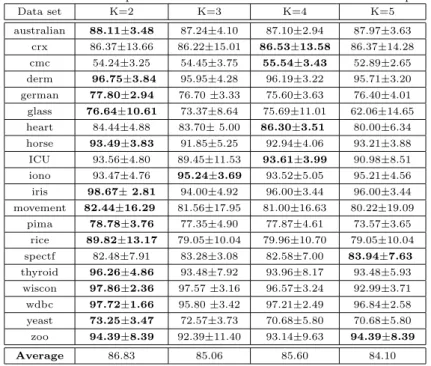
In Table 2, we report the classification performance of DRMF with different random splits. As we can see from there, K has some influence on the perfor-mance of the generated ensembles. Since random splits of the features lead to different rotations, diverse base classifiers are generated. However, if K is too large, the number of features in each subset may become too small and hence not sufficient to effectively represent the learning task, thus leading to a drop in performance. Clearly, a tradeoff between the diversity and the performances of the base classifiers should be made. The experimental results in Table 2 in-dicate that DRMF produces good performance if K= 2, and we consequently set K= 2 in the remainder of experiments.
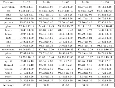
In DRMF, the number of candidate base classifiers should be set before training. Hence, next we investigate how many candidate base classifiers are sufficient to lead to a good ensemble. We thus perform experiments varying the
Table 1: Statistics of classification tasks.
Dataset Instances Discrete Features Continuous Features Classes
australian 690 8 6 2 crx 690 9 6 2 cmc 1473 7 2 3 derm 366 0 34 6 german 1000 13 7 2 glass 214 0 9 6 heart 270 0 13 2 horse 368 15 7 2 ICU 200 16 4 3 iono 351 0 34 2 iris 150 0 4 3 movement 360 0 90 15 pima 768 0 8 2 rice 104 0 5 2 spectf 269 0 44 2 thyroid 215 0 5 3 wiscon 699 0 9 2 wdbc 569 0 30 2 yeast 1484 0 7 2 zoo 101 15 1 7
Table 2: Classification performance of DRMF with different numbers of splits.
Data set K=2 K=3 K=4 K=5 australian 88.11±3.48 87.24±4.10 87.10±2.94 87.97±3.63 crx 86.37±13.66 86.22±15.01 86.53±13.58 86.37±14.28 cmc 54.24±3.25 54.45±3.75 55.54±3.43 52.89±2.65 derm 96.75±3.84 95.95±4.28 96.19±3.22 95.71±3.20 german 77.80±2.94 76.70±3.33 75.60±3.63 76.40±4.01 glass 76.64±10.61 73.37±8.64 75.69±11.01 62.06±14.65 heart 84.44±4.88 83.70±5.00 86.30±3.51 80.00±6.34 horse 93.49±3.83 91.85±5.25 92.94±4.06 93.21±3.88 ICU 93.56±4.80 89.45±11.53 93.61±3.99 90.98±8.51 iono 93.47±4.76 95.24±3.69 93.52±5.05 95.21±4.56 iris 98.67±2.81 94.00±4.92 96.00±3.44 96.00±3.44 movement 82.44±16.29 81.56±17.95 81.00±16.63 80.22±19.09 pima 78.78±3.76 77.35±4.90 77.87±4.61 73.57±3.65 rice 89.82±13.17 79.05±10.04 79.96±10.70 79.05±10.04 spectf 82.48±7.91 83.28±3.08 82.58±7.00 83.94±7.63 thyroid 96.26±4.86 93.48±7.92 93.96±8.17 93.48±5.93 wiscon 97.86±2.36 97.57±3.16 96.57±3.24 92.99±3.71 wdbc 97.72±1.66 95.80±3.42 97.21±2.49 96.84±2.58 yeast 73.25±3.47 72.57±3.73 70.68±5.80 70.68±5.80 zoo 94.39±8.39 92.39±11.40 93.14±9.63 94.39±8.39 Average 86.83 85.06 85.60 84.10
Table 3: Classification performance with different numbers of candidate base classifiers. Data set L=20 L=40 L=60 L=80 L=100 australian 86.96±3.01 88.13±3.98 87.54±2.90 87.97±3.27 88.11±3.48 crx 85.66±14.10 85.51±14.66 85.64±15.10 86.81±13.20 86.37±13.66 cmc 52.82±3.41 53.97±3.30 53.70±3.28 54.18±2.95 54.24±3.25 derm 96.47±3.90 96.98±4.24 95.91±5.26 96.47±4.12 96.75±3.84 german 75.40±3.60 77.00±3.40 77.00±3.02 77.70±2.45 77.80±2.94 glass 72.44±12.14 74.44±11.43 74.89±13.25 78.14±10.91 76.64±10.61 heart 83.33±3.60 83.70±4.68 84.81±4.43 84.81±4.77 84.44±4.88 horse 92.95±4.06 92.94±4.06 93.49±3.38 93.22±3.39 93.49±3.83 ICU 94.04±4.69 94.04±4.69 93.56±4.80 94.09±5.21 93.56±4.80 iono 93.20±4.00 92.92±4.60 93.49±4.95 93.77±5.09 93.47±4.76 iris 94.67±5.26 94.67±5.26 94.67±5.26 96.67±4.71 98.67±2.81 movement 80.56±15.15 82.78±16.50 82.78±16.57 82.44±16.29 82.44±16.29 pima 77.87±4.98 78.52±3.90 78.39±4.53 78.39±4.32 78.78±3.76 rice 89.73±10.18 88.82±10.46 90.73±12.86 89.82±13.17 89.82±13.17 spectf 82.61±5.18 83.34±4.39 82.12±7.21 83.25±7.01 82.48±7.91 thyroid 94.83±6.10 95.30±6.31 94.83±5.21 95.78±5.19 96.26±4.86 wiscon 97.34±2.59 97.43±2.59 97.71±2.15 97.34±2.59 97.86±2.36 wdbc 97.19±2.06 97.72±1.66 98.43±1.53 97.72±1.66 97.72±1.66 yeast 73.11±3.26 73.45±3.12 73.45±3.64 73.38±3.61 73.25±3.47 zoo 94.39±8.39 94.39±8.39 94.39±8.39 94.39±8.39 94.39±8.39 Average 85.78 86.30 86.38 86.82 86.83
number of base classifiers L as 20, 40, 60, 80 and 100, respectively. Table 3 compares the classification performance of DRMF with these settings forL. As we can see from there, the overall performance improves whenLbecomes larger. However, if L> 80, the difference is not significant, and we consequently use L= 100 in the following experiments.
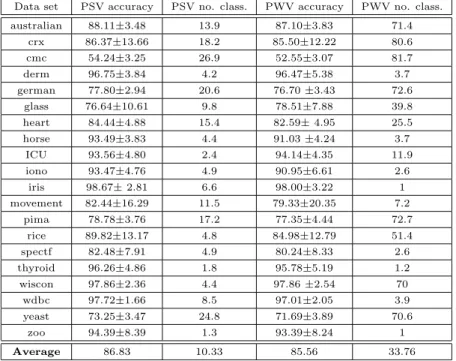
In Margin Based Pruning (Algorithm 2), we utilize simple voting in lines 5 and 9. That is, the class that receives the largest number of votes is considered as the final decision. In contrast, in weighted voting, the votes are weighted and the ensemble decision is the class with the largest sum of weights of votes. Since we calculate the weights in line 2 of Algorithm 2, a natural question that arises is whether applying a weighted voting strategy would give better results. To answer this, we give, in Table 4, the classification accuracies and the number of selected base classifiers2 using the two fusion strategies. From Table 4 we can observe that simple voting performs typically better than weighted voting, while it also leads to smaller ensembles.
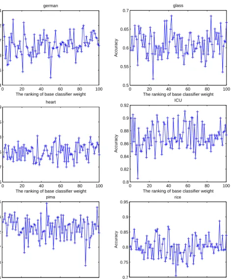
To further investigate why simple voting is better than weighted voting, we perform some additional experiments to explore the relationship between the weights of the base classifiers and their classification performances. Fig. 1 shows the relationship between the classification accuracy and the ranking of
Table 4: Classification performance and number of selected base classifiers for pruned simple voting (PSV) and pruned weighted voting (PWV).
Data set PSV accuracy PSV no. class. PWV accuracy PWV no. class. australian 88.11±3.48 13.9 87.10±3.83 71.4 crx 86.37±13.66 18.2 85.50±12.22 80.6 cmc 54.24±3.25 26.9 52.55±3.07 81.7 derm 96.75±3.84 4.2 96.47±5.38 3.7 german 77.80±2.94 20.6 76.70±3.43 72.6 glass 76.64±10.61 9.8 78.51±7.88 39.8 heart 84.44±4.88 15.4 82.59±4.95 25.5 horse 93.49±3.83 4.4 91.03±4.24 3.7 ICU 93.56±4.80 2.4 94.14±4.35 11.9 iono 93.47±4.76 4.9 90.95±6.61 2.6 iris 98.67±2.81 6.6 98.00±3.22 1 movement 82.44±16.29 11.5 79.33±20.35 7.2 pima 78.78±3.76 17.2 77.35±4.44 72.7 rice 89.82±13.17 4.8 84.98±12.79 51.4 spectf 82.48±7.91 4.9 80.24±8.33 2.6 thyroid 96.26±4.86 1.8 95.78±5.19 1.2 wiscon 97.86±2.36 4.4 97.86±2.54 70 wdbc 97.72±1.66 8.5 97.01±2.05 3.9 yeast 73.25±3.47 24.8 71.69±3.89 70.6 zoo 94.39±8.39 1.3 93.39±8.24 1 Average 86.83 10.33 85.56 33.76
their weights. Here, the x-axis indicates the ranking of the weight with 1 indi-cating the largest weight of the base classifier and 100 the smallest. From Fig. 1 we can conclude that base classifiers with large weights do not necessarily have better classification performance compared to those with small weights. Weight learning considers both the diversity among base classifiers and their perfor-mances and hence while the weights can be used to rank the base classifiers, they do not reflect their classification performances.
In our algorithm, the base classifiers are added to the ensemble one by one. Base classifiers with the large weights are included first. Fig. 2 plots the clas-sification accuracies when the base classifiers are added, for both simple and weighted voting. From there, we can notice that the best classification accuracy obtained by simple voting is often higher than that of weighted voting, confirm-ing that simple votconfirm-ing can produce better performance than weighted votconfirm-ing. We can also see that fusion based on only a subset of base classifiers is better than combining all of them, which is consistent with the findings from [55].
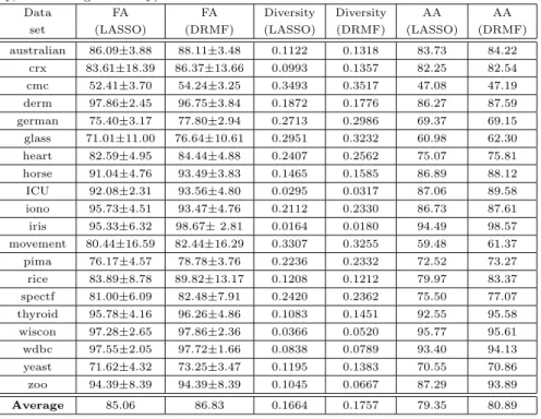
Margin Based Pruning has two main components. One is to learn the weights for the base classifiers via the minimization ofJW, while the other is to select the base classifiers. Some of the weights might be zero, and we consequently tested whether the classification performance is affected if we remove base classifier with zero weights. For this, in Table 5, we compare the fusion accuracy of base classifiers that receive non-zero weights (denoted by LASSO in Table 5)
0 20 40 60 80 100 0.64 0.66 0.68 0.7 0.72 0.74
The ranking of base classifier weight
Accuracy german 0 20 40 60 80 100 0.5 0.55 0.6 0.65 0.7
The ranking of base classifier weight
Accuracy glass 0 20 40 60 80 100 0.65 0.7 0.75 0.8 0.85 0.9
The ranking of base classifier weight
Accuracy heart 0 20 40 60 80 100 0.8 0.82 0.84 0.86 0.88 0.9 0.92
The ranking of base classifier weight
Accuracy ICU 0 20 40 60 80 100 0.66 0.68 0.7 0.72 0.74 0.76
The ranking of base classifier weight
Accuracy pima 0 20 40 60 80 100 0.7 0.75 0.8 0.85 0.9 0.95
The ranking of base classifier weight
Accuracy
rice
Figure 1: Classification accuracies of base classifiers with different ranking in terms of their weights.
with the fusion accuracy of DRMF. It can be seen that DRMF performs better than LASSO, and thus that Steps 3 to 8 in Algorithm 2 are indeed useful for improving the classification performance. We also analyze the differences between the base classifiers selected by the two strategies. From Table 5 it is apparent that the average accuracy of the base classifiers in DRMF is higher than that of the base classifiers that receive non-zero weights, and the diversity among base classifiers in DRMF is also higher than that of the base classifiers with non-zero weights.
0 20 40 60 80 100 0.72 0.73 0.74 0.75 0.76 0.77 0.78 0.79 0.8
Number of fused base classifiers
Accuracy german simple voting weight voting 0 20 40 60 80 100 0.65 0.7 0.75 0.8
Number of fused base classifiers
Accuracy glass simple voting weight voting 0 20 40 60 80 100 0.76 0.78 0.8 0.82 0.84 0.86
Number of fused base classifiers
Accuracy heart simple voting weight voting 0 20 40 60 80 100 0.88 0.89 0.9 0.91 0.92 0.93 0.94
Number of fused base classifiers
Accuracy ICU simple voting weight voting 0 20 40 60 80 100 0.73 0.74 0.75 0.76 0.77 0.78 0.79 0.8 0.81
Number of fused base classifiers
Accuracy pima simple voting weight voting 0 20 40 60 80 100 0.83 0.84 0.85 0.86 0.87 0.88 0.89 0.9 0.91
Number of fused base classifiers
Accuracy
rice
simple voting weight voting
Figure 2: Variation of classification accuracies with different numbers of selected base classi-fiers when simple voting and weighted voting are used.
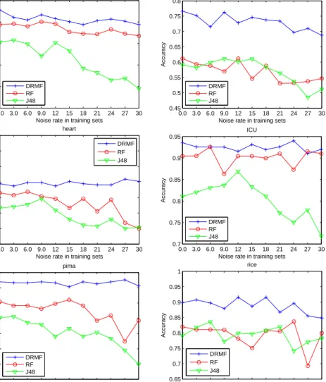
and J48. For that, we first generate noisy samples by randomly revising the labels of some training samples with the percentage of relabeled samples varying from 3% to 30%. Fig. 3 shows the variation of classification accuracies when we increase the noise rate in the training set. As is apparent, DRMF shows superior robustness compared to both Rotation Forest and J48. In particular, for DRMF the variation of the classification accuracies remains small as the rate of mislabeled samples increases.
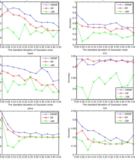
We further consider the robustness of the algorithms with respect to at-tribute noise and add Gaussian noise to the features of the training data. The
Table 5: Comparison of different strategies used in selecting base classifiers (FA=fusion accu-racy, AA=average accuracy).
Data FA FA Diversity Diversity AA AA
set (LASSO) (DRMF) (LASSO) (DRMF) (LASSO) (DRMF)
australian 86.09±3.88 88.11±3.48 0.1122 0.1318 83.73 84.22 crx 83.61±18.39 86.37±13.66 0.0993 0.1357 82.25 82.54 cmc 52.41±3.70 54.24±3.25 0.3493 0.3517 47.08 47.19 derm 97.86±2.45 96.75±3.84 0.1872 0.1776 86.27 87.59 german 75.40±3.17 77.80±2.94 0.2713 0.2986 69.37 69.15 glass 71.01±11.00 76.64±10.61 0.2951 0.3232 60.98 62.30 heart 82.59±4.95 84.44±4.88 0.2407 0.2562 75.07 75.81 horse 91.04±4.76 93.49±3.83 0.1465 0.1585 86.89 88.12 ICU 92.08±2.31 93.56±4.80 0.0295 0.0317 87.06 89.58 iono 95.73±4.51 93.47±4.76 0.2112 0.2330 86.73 87.61 iris 95.33±6.32 98.67±2.81 0.0164 0.0180 94.49 98.57 movement 80.44±16.59 82.44±16.29 0.3307 0.3255 59.48 61.37 pima 76.17±4.57 78.78±3.76 0.2236 0.2332 72.52 73.27 rice 83.89±8.78 89.82±13.17 0.1208 0.1212 79.97 83.37 spectf 81.00±6.09 82.48±7.91 0.2420 0.2362 75.50 77.07 thyroid 95.78±4.16 96.26±4.86 0.1083 0.1451 92.55 95.58 wiscon 97.28±2.65 97.86±2.36 0.0366 0.0520 95.77 95.61 wdbc 97.55±2.05 97.72±1.66 0.0838 0.0789 93.40 94.13 yeast 71.62±4.32 73.25±3.47 0.1195 0.1383 70.55 70.86 zoo 94.39±8.39 94.39±8.39 0.1045 0.0667 87.29 93.89 Average 85.06 86.83 0.1664 0.1757 79.35 80.89
mean of the noise is zero, while we vary the standard deviation from 0 to 0.5, and show the results in Fig. 4. As we can observe from there, DRMF is more ro-bust with respect to attribute noise than J48, and performs similarly compared to Rotation Forest.
5. Simulation and Experimental Analysis
In this section, we compare DRMF with some other representative classifica-tion algorithms including J48, Rotaclassifica-tion Forest, AdaBoostM1,and Bagging, on the 20 datasets from Table 1. For all ensembles, base classifiers are generated using J48. For DRMF and Rotation Forest, we setK= 2, the rate of bootstrap sampling to 0.75 and the numberLof base classifiers to 100. The parameters of Bagging and AdaBoostM1 were kept as their default values in WEKA, while the number of base classifiers was also set to 100. We performed standard 10-fold cross validation to compute the classification performance. Table 6 gives the classification accuracies on all datasets together with the standard deviations for all evaluated algorithms.
We further employ a test for statistical significance, namely the Nemenyi test [37], to compare the algorithms. In this test, the critical difference [16] for
0.0 3.0 6.0 9.0 12 15 18 21 24 27 30 0.55 0.6 0.65 0.7 0.75 0.8
Noise rate in training sets
Accuracy german DRMF RF J48 0.0 3.0 6.0 9.0 12 15 18 21 24 27 30 0.45 0.5 0.55 0.6 0.65 0.7 0.75 0.8
Noise rate in training sets
Accuracy glass DRMF RF J48 0.0 3.0 6.0 9.0 12 15 18 21 24 27 30 0.65 0.7 0.75 0.8 0.85 0.9 0.95 1
Noise rate in training sets
Accuracy heart DRMF RF J48 0.0 3.0 6.0 9.0 12 15 18 21 24 27 30 0.7 0.75 0.8 0.85 0.9 0.95
Noise rate in training sets
Accuracy ICU DRMF RF J48 0.0 3.0 6.0 9.0 12 15 18 21 24 27 30 0.66 0.68 0.7 0.72 0.74 0.76 0.78 0.8
Noise rate in training sets
Accuracy pima DRMF RF J48 0.0 3.0 6.0 9.0 12 15 18 21 24 27 30 0.65 0.7 0.75 0.8 0.85 0.9 0.95 1
Noise rate in training sets
Accuracy
rice
DRMF RF J48
Figure 3: Variation of classification accuracies when varying the rate of class noise.
the five algorithms and 20 data sets at significance levelα= 0.05 is CD=q0.05 r k(k+ 1) 6N = 2.728× r 5×(5 + 1) 6×20 = 1.364, (18)
whereq0.05is the critical value for the two-tailed Nemenyi test,kis the number of the algorithms andNis the number of data sets.
The average ranks for DRMF, J48, Bagging, AdaBoostM1 and Rotation Forest were thus found to be 1.55, 4.36, 3.00, 3.05, and 3.03, respectively, and the average rank differences between DRMF and the other methods were 4.375−
0.00 0.05 0.10 0.15 0.20 0.25 0.30 0.35 0.40 0.45 0.50 0.66 0.68 0.7 0.72 0.74 0.76 0.78
The standard deviation of Gaussian noise
Accuracy german DRMF RF J48 0.00 0.05 0.10 0.15 0.20 0.25 0.30 0.35 0.40 0.45 0.50 0.2 0.3 0.4 0.5 0.6 0.7 0.8 0.9 1
The standard deviation of Gaussian noise
Accuracy glass DRMF RF J48 0.00 0.05 0.10 0.15 0.20 0.25 0.30 0.35 0.40 0.45 0.50 0.65 0.7 0.75 0.8 0.85 0.9
The standard deviation of Gaussian noise
Accuracy heart DRMF RF J48 0.00 0.05 0.10 0.15 0.20 0.25 0.30 0.35 0.40 0.45 0.50 0.75 0.8 0.85 0.9 0.95
The standard deviation of Gaussian noise
Accuracy ICU DRMF RF J48 0.00 0.05 0.10 0.15 0.20 0.25 0.30 0.35 0.40 0.45 0.50 0.55 0.6 0.65 0.7 0.75 0.8
The standard deviation of Gaussian noise
Accuracy pima DRMF RF J48 0.00 0.05 0.10 0.15 0.20 0.25 0.30 0.35 0.40 0.45 0.50 0.7 0.75 0.8 0.85 0.9 0.95
The standard deviation of Gaussian noise
Accuracy
rice
DRMF RF J48
Figure 4: Variation of classification accuracies when varying the rate of attribute noise.
and 3.025−1.55 = 1.475>1.364. Consequently, DRMF was shown to perform statistically significantly better than all other methods.
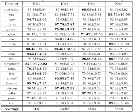
Next, we discuss why, compared with Rotation Forest, DRMF is able to further boost the classification performance. First, it can be seen that the pa-rameterKin DRMF and Rotation Forest was set to 2 in the above experiments. From Table 2 we know, that K = 2 is suitable for DRMF. In order to verify whether K = 2 is also suitable for Rotation Forest, the classification perfor-mances of Rotation Forest with different numbers of splits are given in Table 7. From there, we can see that Rotation Forest also produces good performance if K= 2.
Table 6: Performance comparison with other classifiers.
Data set DRMF J48 Bagging AdaBoostM1 Rotation Forest
australian 88.11±3.48 83.05±5.40 86.55±6.07 86.10±5.01 85.83±5.09 crx 86.37±13.66 82.74±13.38 83.91±15.48 85.21±12.94 83.04±17.89 cmc 54.24±3.25 54.65±2.65 53.84±3.32 50.24±2.49 54.72±2.62 derm 96.75±3.84 93.73±4.50 96.39±3.72 95.12±3.30 97.10±3.19 german 77.80±2.94 70.30±3.40 75.60±3.17 76.00±3.53 74.40±4.79 glass 76.64±10.61 59.11±13.53 68.17±11.17 72.89±17.04 61.17±11.68 heart 84.44±4.88 76.67±5.25 82.22±7.77 80.00±5.84 81.48±6.98 horse 93.49±3.83 96.19±2.65 97.27±2.27 97.56±0.86 91.02±4.64 ICU 93.56±4.80 81.03±29.12 84.14±29.72 84.14±29.83 90.45±12.03 iono 93.47±4.76 89.24±7.90 91.21±5.83 93.22±4.62 94.34±4.94 iris 98.67±2.81 96.00±3.44 94.67±6.13 96.00±3.44 95.33±3.22 movement 82.44±16.29 62.44±16.89 68.89±17.73 74.11±18.82 82.00±20.92 pima 78.78±3.76 74.09±5.87 76.43±4.89 73.57±3.74 76.17±3.39 rice 89.82±13.17 79.05±10.04 83.89±8.78 83.89±8.78 81.98±8.95 spectf 82.48±7.91 73.47±8.47 78.78±10.74 78.46±9.85 80.26±6.15 thyroid 96.26±4.86 93.48±5.93 94.87±6.43 94.00±10.12 95.78±7.25 wiscon 97.86±2.36 94.57±2.10 96.43±3.03 95.71±3.01 96.57±2.87 wdbc 97.72±1.66 92.98±3.96 96.31±3.36 97.19±1.90 97.19±2.22 yeast 73.25±3.47 74.53±4.44 76.68±5.55 73.52±3.59 71.89±3.88 zoo 94.39±8.39 90.76±10.26 93.30±7.07 96.38±5.75 90.65±9.13
Table 7: Classification performances of RF with different numbers of splits.
Data set K=2 K=3 K=4 K=5 australian 85.83±5.09 85.80±3.83 86.09±3.53 84.34±3.62 crx 83.04±17.89 82.18±17.54 82.89±15.68 83.75±16.00 cmc 54.72±2.62 52.68±2.60 53.02±4.37 52.89±2.65 derm 97.10±3.19 97.78±2.87 97.26±2.93 97.02±2.99 german 74.40±4.79 75.30±3.97 75.10±5.09 74.80±4.87 glass 61.17±11.68 66.33±10.64 71.42±13.53 60.22±15.34 heart 81.48±6.98 84.81±4.08 83.33±6.11 77.41±9.31 horse 91.02±4.64 91.84±3.66 91.56±3.77 92.66±3.39 ICU 90.45±12.03 90.45±13.92 87.29±17.86 87.29±21.75 iono 94.34±4.94 93.50±4.95 94.06±5.21 93.50±4.95 iris 95.33±3.22 94.00±4.92 96.00±3.44 96.00±3.44 movement 82.00±20.92 80.89±21.25 78.11±23.44 80.33±20.03 pima 76.17±3.39 75.13±5.20 74.74±5.04 73.57±3.65 rice 81.98±8.95 79.05±10.04 79.96±10.70 79.05±10.04 spectf 80.26±6.15 80.99±7.46 78.86±7.67 81.01±5.52 thyroid 95.78±7.25 93.48±7.92 93.96±8.17 93.48±5.93 wiscon 96.57±2.87 97.43±2.92 96.00±3.29 92.99±3.71 wdbc 97.19±2.22 97.38±2.64 97.73±2.33 97.02±2.62 yeast 71.89±3.88 70.55±5.80 70.68±5.80 70.68±6.05 zoo 90.65±9.13 90.28±8.34 88.65±9.04 92.39±9.24 Average 84.07 83.99 83.84 83.02
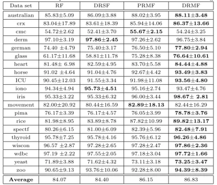
Table 8: Classification performances with different rotation and fusion strategies. Data set RF DRSF PRMF DRMF australian 85.83±5.09 86.09±3.88 88.02±3.95 88.11±3.48 crx 83.04±17.89 83.61±18.39 85.94±14.06 86.37±13.66 cmc 54.72±2.62 52.41±3.70 55.67±2.15 54.24±3.25 derm 97.10±3.19 97.86±2.45 97.26±2.62 96.75±3.84 german 74.40±4.79 75.40±3.17 76.50±5.10 77.80±2.94 glass 61.17±11.68 58.81±11.78 75.28±8.38 76.64±10.61 heart 81.48±6.98 82.59±4.95 83.70±5.58 84.44±4.88 horse 91.02±4.64 91.04±4.76 92.67±4.42 93.49±3.83 ICU 90.45±12.03 91.55±3.34 91.98±11.08 93.56±4.80 iono 94.34±4.94 95.73±4.51 95.16±2.74 93.47±4.76 iris 95.33±3.22 95.33±6.32 96.00±3.44 98.67±2.81 movement 82.00±20.92 80.44±16.59 82.89±18.13 82.44±16.29 pima 76.17±3.39 76.17±4.57 76.05±3.99 78.78±3.76 rice 81.98±8.95 83.89±8.78 87.82±10.99 89.82±13.17 spectf 80.26±6.15 81.00±6.09 82.39±5.96 82.48±7.91 thyroid 95.78±7.25 95.78±4.16 95.76±6.12 96.26±4.86 wiscon 96.57±2.87 97.28±2.65 97.28±2.47 97.86±2.36 wdbc 97.19±2.22 97.55±2.05 97.18±3.04 97.72±1.66 yeast 71.89±3.88 71.62±4.32 73.11±3.18 73.25±3.47 zoo 90.65±9.13 93.76±10.06 92.28±8.00 94.39±8.39 Average 84.07 84.40 86.15 86.83
The difference between DRMF and Rotation Forest mainly comprises two parts: the use of Double Rotation to generate the base classifiers, and Margin Based Pruning. Thus, we explore whether they are both necessary for improving the classification performance of the ensemble. For this, we test four combina-tions: Rotation Forest (RF); a combination of Double Rotation and the fusion strategy in Rotation Forest i.e. simple voting of all base classifiers (DRSF), a combination of PCA rotation and Margin Based Pruning (PRMF), and DRMF. The results are presented in Table 8. As we can confirm from there, both Dou-ble Rotation and Margin Based Pruning are indeed useful for improving the classification performance.
Further, we compute the margin distribution of the ensembles generated using the above four classification algorithms, where the margin of a sample is computed as the difference between the number of correct votes and the maximum number of the votes received by any wrong label [42]. A large margin is understood as a “confident” classification, and thus we would desire that large margins of the training samples are derived. Fig. 5 shows the margin distribution when RF, DRSF, PRMF and DRMF are used. We can observe, that compared with RF, DRMF improves the margin distribution on the training set, which confirms that both Double Rotation and Margin Based Pruning are helpful for improving the margin distribution.
So, why does Double Rotation improve the margin distribution of the train-ing set? From Theorem 1, we know that the margin of the traintrain-ing samples has
−1 −0.5 0 0.5 1 0 0.2 0.4 0.6 0.8 1
margin of training samples
cumulative frequency german DRMF DRSF PRMF RF −1 −0.5 0 −0.05 0 0.05 0.1 −1 −0.5 0 0.5 1 0 0.2 0.4 0.6 0.8 1
margin of training samples
cumulative frequency glass DRMF DRSF PRMF RF −1 −0.5 0 −0.04 −0.02 0 0.02 −1 −0.5 0 0.5 1 0 0.2 0.4 0.6 0.8 1
margin of training samples
cumulative frequency heart DRMF DRSF PRMF RF −1 −0.5 0 −0.04 −0.02 0 0.02 −1 −0.5 0 0.5 1 0 0.2 0.4 0.6 0.8 1
margin of training samples
cumulative frequency ICU DRMF DRSF PRMF RF −1 −0.5 0 −0.04 −0.02 0 0.02 −1 −0.5 0 0.5 1 0 0.2 0.4 0.6 0.8 1
margin of training samples
cumulative frequency pima DRMF DRSF PRMF RF −1 −0.5 0 −0.05 0 0.05 0.1 −1 −0.5 0 0.5 1 0 0.2 0.4 0.6 0.8 1
margin of training samples
cumulative frequency rice DRMF DRSF PRMF RF −1 −0.5 0 −0.05 0 0.05
Figure 5: Margin cumulative frequency of training samples for RF, DRSF, PRMF and DRMF.
an underlying relationship with the diversity of the base classifiers. We thus compare the diversity of the base classifiers when employing Double Rotation and PCA rotation, and show the results in Fig. 6. From there we can notice that the diversity among base classifiers is consistently enhanced after Double Rotation. However, from Fig. 7 we see that the average accuracies of the two kinds of base classifiers are almost the same. Consequently, we can derive that the improvements of the margin distribution come from the diversity, and not from the improved accuracies of the base classifiers.
Finally, we conducted some experiments to validate the effectiveness of the proposed Margin Based Pruning (Margin-P) algorithm and compared it with
australian crx cmc derm german glass heart horse ICU iono irismovementpima rice spectf thyroidwiscon wdbc yeast zoo 0 0.02 0.04 0.06 0.08 0.1 0.12 0.14 0.16 0.18 Diversity Double rotation PCA rotation
Figure 6: Diversity of Double Rotation and PCA Rotation.
other ensemble pruning techniques based on the margin including MeanD-M [52] and the improved version of MDM [32, 33]. MeanD-M optimizes the average margin via a backward elimination strategy. In particular, it ranks the contri-bution and importance of every base classifier Cj in the temporary ensemble Γ by observing the decrease of the average margin when removingCjfrom the en-semble. During each step, the least important classifierCminwith the minimum decrease of the average margin is eliminated from the ensemble and the ensem-ble thus shrinks to its subset Γ′
= Γ\ Cmin. Then, the base classifiers in Γ ′
are reordered and the above process is repeated. MDM selects base classifiers via a forward selection strategy where base classifiers are sequentially added based on a specified rule. In particular, the classifier selected in theu-th iteration is
su= arg min j d(o, 1 u(cj+ u−1 X t=1 cst)), (19)
where cj is the N-dimensional signature vector of Cj whose i-th component (cj)i is 1 if the sample xi is correctly classified by Cj and is -1 otherwise. j runs through the classifiers outside the temporary ensemble and d(v1,v2) is the distance between vectorsv1 and v2. In [33], the objective pointois placed in the first quadrant with equal componentsoi=p(e.g.,p= 0.075). An improved version of MDM is proposed [32], which uses a moving objective point o that allowsp(u) to vary with the size of the sub-ensembleu. Exploratory experiments show that a value p(u)∝√uis appropriate. improved version for comparison with our method.
australian crx cmc derm germanglass heart horse ICU iono irismovementpima rice spectf thyroidwiscon wdbc yeast zoo 0.5 0.6 0.7 0.8 0.9 1 Accuracy
Different data sets Box plots of classification accuracies with Double rotation
australian crx cmc derm german glass heart horse ICU iono irismovementpima rice spectf thyroidwiscon wdbc yeastzoo 0.45 0.5 0.55 0.6 0.65 0.7 0.75 0.8 0.85 0.9 0.95 Accuracy
Different data sets Box plots of classification accuracies with PCA rotation
Figure 7: Box plots of classification accuracies with different rotation strategies.
In MeanD-M, base classifiers are eliminated from the original ensemble one by one and the sub-ensemble with the best accuracy on the test set is used to estimate its performance. Thus, we also use the best accuracy on the test set to estimate the classification performance for MDM and Margin-P. The results of the experiment are given in Table 9. From there, we can confirm that our algorithm does indeed performs better than the pruning strategies in most cases.
6. Conclusions and Future Work
Ensemble learning is an effective approach to improve the generalization performance of a classification system. In this paper, we have proposed Double
Table 9: The best test performances based on different pruning methods.
Data set MeanD-M MDM Margin-P
australian 88.41±3.48 87.54±2.99 88.98±3.16 crx 86.22±15.11 87.23±14.20 87.81±13.71 cmc 55.94±2.97 56.08±4.00 56.62±3.48 derm 98.41±2.21 98.13±2.16 98.41±2.21 german 78.60±2.17 79.00±2.49 79.50±3.06 glass 77.60±10.62 75.24±7.89 79.94±9.89 heart 86.30±3.92 85.93±4.55 87.04±3.15 horse 94.59±4.37 93.50±3.64 94.85±3.70 ICU 93.61±5.31 94.56±5.06 94.61±4.29 iono 97.12±3.66 96.60±3.71 96.84±3.27 iris 98.00±4.50 97.33±3.44 98.67±2.81 movement 85.33±16.04 83.67±16.06 85.44±15.87 pima 78.91±3.15 79.43±4.10 80.86±3.39 rice 91.55±8.24 91.34±8.29 94.36±6.48 spectf 85.86±4.25 85.11±7.27 86.62±5.56 thyroid 97.19±4.58 96.69±4.51 97.64±4.62 wiscon 98.00±2.25 98.43±1.96 98.14±2.13 wdbc 98.60±1.38 98.25±1.42 98.42±1.29 yeast 73.92±3.41 74.12±4.08 74.46±2.32 zoo 95.39±8.41 95.39±8.41 95.39±8.41 Average 87.98 87.68 88.73
Rotation Margin Forest (DRMF) as an effective new ensemble learning algo-rithm. The idea of DRMF is to improve the generalization performance by improving the margin distribution on the training set. Extensive experimental results on 20 benchmark datasets confirm that DRMF provides a competent en-semble learner, and allows us to draw several conclusions: (1) Double Rotation with PCA and LSDA is able to generate diverse base classifiers; (2) The margin distribution of the ensemble system is improved if a set of diverse base clas-sifiers is exploited by optimizing a regularized loss function, and consequently the classification performance of the ensemble is enhanced; (3) The DRMF al-gorithm outperforms classical ensemble learning techniques such as Bagging, AdaBoostM1 and Rotation Forest.
Our work is motivated by the idea that diversity among base classifiers can improve the margin distribution of the ensemble. However, no deep discussion on this issue has been reported so far. Further theoretical analysis on the relationship between diversity and margin is thus required. While in this paper, we use Double Rotation to create diversity, some other techniques could also be introduced. A systematic discussion on generating diversity would therefore present an important task. Although DRMF is presented as an approach to create homogenous ensembles (e.g., based only on decision trees as the base classifiers), it is straightforward to use DRMF to learn and prune heterogeneous classifiers for ensemble learning. Exploring the effectiveness of DRMF in such a setting might be an interesting avenue.
Acknowledgments
This work is supported by the National Program on Key Basic Research Project under Grant 2013CB329304, National Natural Science Foundation of China under Grants 61222210, 60873140, 61170107, 61073125, 61071179, 60963006, and 11078010, National Science Fund for Distinguished Young Scholars under Grant 50925625 and the Program for New Century Excellent Talents in Univer-sity (No. NCET-12-0399, NCET-08-0155, and NCET-08-0156).
References
[1] M. Aksela and J. Laaksonen, Using diversity of errors for selecting members of a committee classifier, Pattern Recognition, 39 (2006) 608-623.
[2] F. Aiolli and A. Sperduti, A re-weighting strategy for improving margins, Artificial Intelligence, 137 (2002) 197-216.
[3] C. Blake, E. Keogh and C. J. Merz (1998), UCI Repository of Machine Learning Databases. Dept. Inf. Comput. Sci., Univ. California, Irvine, CA. [Online]. Available: http://www.ics.uci.edu/ mlearn/MLRepository. html. [4] L. Breiman, Bagging predictors, Machine Learning, 24 (1996) 123-140. [5] L. Breiman, Stacked regressions, Machine Learning, 24 (1996) 49-64. [6] P. L. Bartlett, For valid generalization, the size of the weights is more
important than the size of the network, In Advances inNeural Information Processing Systems, vol. 9, 1997.
[7] R. Bryll, R. Gutierrez-Osuna and F. Quek, Attribute bagging: improving accuracy of classifier ensembles by using random feature subsets, Pattern Recognition, 36 (2003) 1291-1302.
[8] B. E. Boser, I. M. Guyon and V. N. Vapnik, A training algorithm for opti-mal margin classifiers, In Proceedings of the Fifth Annual ACM Workshop on Computational Learning Theory, pp. 144-152, 1992.
[9] J. A. Benediktsson, J. R. Sveinsson, O. K. Ersoy and P. H. Swain, Parallel consensual neural networks, IEEE Transactions on Neural Networks, 8 (1) (1997) 54-64.
[10] K. J. Cherkauer, Human expert level performance on a scientific image analysis task by a system using combined artificial neural networks, in: Proceedings of 13th AAAI workshop on integrating multiple learned models for improving and scaling machine algorithms, pp. 15-21, 1996.
[11] K. Crammer, R. Gilad-Bachrach, A. Navot and A. Tishby, Margin analysis of the LVQ algorithm, Advances in Neural Information Processing Systems, 15 (2003) 462-469.
[12] D. Cai, X. F. He, K. Zhou, J. W. Han and H. J. Bao, Locality Sensitive Discriminant Analysis, International Joint Conference on Artificial Intelli-gence, pp. 708-713, 2007.
[13] H. Chen, P. Tino and X. Yao, Predictive ensemble pruning by expectation propagation, IEEE Transactions on Knowledge and Data Engineering, 21 (7) (2009) 999-1013.
[14] C. Cortes and V. Vapnik, Support-vector networks, Machine Learning, 20 (3) (1995) 273-297.
[15] Q. Dai, A competitive ensemble pruning approach based on cross-validation technique, Knowledge-Based Systems, 37 (2013) 394-414.
[16] J. Demˇsar, Statistical comparisons of classifiers over multiple data sets, Journal of Machine Learning Research, 7 (1) (2006) 1-30.
[17] Y. Freund, Boosting a weak learning algorithm by majority, Information and computation, 121 (1996) 256-285.
[18] S. Floyd and M. Marmuth, Sample compression learnability, and the Vap-nikC Chervonenkis dimension, Machine Learning, 21 (3) (1995) 269-304. [19] G. Fumera and F. Roli, A theoretical and experiment alanalysis of linear
combiners for multiple classifier systems, IEEE Transactions on Pattern Analysis and Machine Intelligence, 27 (6) (2005) 942-956.
[20] Y. Freund and R. E. Schapire, A decision-theoretic generalization of online learning and an application to boosting, J. Comput. Syst. Sci., 55 (1) (1997) 119-139.
[21] Y. Freund and R. E. Schapire, Large Margin Classification Using the Per-ceptron Algorithm, Machine Learning, 37 (3) (1999) 277-296.
[22] T. Graepel, R. Herbrich and J. Shawe-Taylor, Generalization error bounds for sparse linear classifiers, in: 13th Annual Conference on Computational Learning Theory, pp. 298-303, 2000.
[23] A. J. Grove and D. Schuurmans, Boosting in the limit: maximizing the mar-gin of learned ensembles, in:Proceedings of the 15th National Conference on Artificial Intelligence,American Association for Artificial Intelligence, Menlo Park, CA, USA, pp. 692-699, 1998.
[24] D. Hern´andez-Lobato, G. Mart´ınez-Mu˜noz and A. Su´arez, Empirical analy-sis and evaluation of approximate techniques for pruning regression bagging ensembles, Neurocomputing, 74 (12-13) (2011) 2250-2264.
[25] Q. H. Hu, D. R. Yu and M. Y. Wang, Constructing Rough Decision Forests, D. Slezak et al. (Eds.), RSFDGrC 2005, Lecture Notes in Artificial Intelli-gence, 3642 (2005) 147-156.
[26] Q. H. Hu, P. F. Zhu, Y. B. Yang and D. R. Yu, Large-margin nearest neighbor classifiers via sample weight learning, Neurocomputing, 74 (2011) 656-660.
[27] M. Hall, E. Frank, G. Holmes, B. Pfahringer, P. Reutemann and I. H. Witten, The WEKA Data Mining Software: An Update, SIGKDD Explo-rations, 11 (1) (2009) 10-18.
[28] J. Kittler, M. Hatef, R. P. W. Duin and J. Matas, On combining classifiers, IEEE Transactions on Pattern Analysis and Machine Intelligence, 20 (3) (1998) 226-239.
[29] L. I. Kuncheva, Switching Between Selection and Fusion in Combining Classifiers: An Experiment, IEEE Transactions on Systems, Man and Cy-bernetics, Part-B: CyCy-bernetics, 32 (2) (2002) 146-156.
[30] L. Kuncheva and C. Whitaker, Measures of diversity in classifier ensembles and their relationship with the ensemble accuracy, Machine Learning, 51 (2003) 181-207.
[31] D. D. Margineantu and T. G. Dietterich, Pruning adaptive boosting, in: Proceedings of the 14th International Conference on Machine Learning, Morgan Kaufmann Publishers Inc.,San Francisco, CA, USA, pp. 211-218, 1997.
[32] G. Mart´ınez-Mu˜noz, D. Hernandez-Lobato and A.Suarez, An analysis of ensemble pruning techniques based on ordered aggregation, IEEE Transac-tions on Pattern Analysis and Machine Intelligence, 31 (2) (2009) 245-259. [33] G. Mart´ınez-Mu˜noz and A. Su´arez, Aggregation ordering in bagging, in:Proceedings of the International Conference on Artificial Intelligence and Applications, pp. 258-263, 2004.
[34] G. Mart´ınez-Mu˜noz and A. Su´arez, Pruning in ordered bagging ensembles, in: Proceedings of the 23th International Conference on Machine Learning, pp. 609-616, 2006.
[35] G. Mart´ınez-Mu˜noz and A. Su´arez, Using boosting to prune bagging en-sembles, Pattern Recognition Letters, 28 (1) (2007) 156-165.
[36] R. Maclin and J. W. Shavlik, Combining the predictions of multiple clas-sifiers: using competitive learning to initialize neural networks, in: Pro-ceedings of the 14th international joint conference on artificial intelligence, Morgan Kaufmann, San Mateo, CA, pp. 524-530, 1995.
[37] P. B. Nemenyi. Distribution-free multiple comparisons, PhD thesis, Prince-ton University, 1963.
[38] A. Rahman and B. Verma, Ensemble classifier generation using non-uniform layered clustering and Genetic Algorithm, Knowledge-Based Sys-tems 43 (2013) 30-42.
[39] J. J. Rodr´ıguez and L. I. Kuncheva, Rotation Forest: A New Classifier Ensemble Method, IEEE Transactions on Pattern Analysis and Machine Intelligence, 28 (10) (2006) 1619-1630.
[40] S. Rosset, Z. Ji and T. Hastie, Boosting as a regularized path to a maximum margin classifier, Journal of Machine learning research, 5 (2004) 941-973. [41] R. E. Schapire, The strength of weak learnability, Machine Learning, 5
(1990) 197-227.
[42] R. E. Schapire, Y. Freund, P. Bartlett and W. S. Lee, Boosting the margin: A new explanation for the effectiveness of voting methods, The Annals of Statistics, 26 (5) (1998) 1651-1686.
[43] J. Shawe-Taylor, P. L. Bartlett, R. C. Williamson and M. Anthony, A framework for structural risk minimisation, In Proceedings of the Ninth Annual Conference on Computational Learning Theory, pp. 68-76, 1996. [44] J. Shawe-Taylor and N. Cristianini, Margin Distribution Bounds on
Gen-eralization, EuroCOLT 1999, pp. 263-273.
[45] C. H. Shen and H. X. Li, Boosting Through Optimization of Margin Distri-butions, IEEE Transactions on Neural Networks, vol. 21 (4) (2010) 659-666. [46] E. K. Tang, P. N. Suganthan and X. Yao, An analysis of diversity measures,
Machine Learning, 65 (2006) 247-271.
[47] R. Tibshirani, Regression shrinkage and selection via the lasso, J. Royal. Statist. Soc B. 58 (1) (1996) 267-288.
[48] N. Ueda, Optimal linear combination of neural networks for improving classification performance, IEEE Transactions on Pattern Analysis and Ma-chine Intelligence, 22 (2) (2000) 207-215.
[49] V. N. Vapnik, Estimation of Dependences Based on Empirical Data, Springer-Verlag, New York, 1982.
[50] K. Weinberger, J. Blitzer and L. Saul, Distance metric learning for large margin nearest neighbor classification, Advances in Neural Information Processing Systems (NIPS), 18 (2006) 1473-1480.
[51] L. W. Wang, M. Sugiyama, Z. X. Jing, C. Yang, Z. H. Zhou and J. F. Feng, A Refined Margin Analysis for Boosting Algorithms via Equilibrium Margin, Journal of Machine Learning Research, 12 (2011) 1835-1863. [52] F. Yang, W. H. Lu, L. K. Luo and T. Li, Margin optimization based pruning
for random forest, Neurocomputing, 94 (2012) 54-63.
[53] X. Yao and Y. Liu, Making use of population information in evolution-ary artificial neural networks, IEEE Transactions on Systems, Man and Cybernetics, Part-B: Cybernetics, 28 (3) (1998) 417-425.
[54] Y. Zhang, S. Burer and W. N. Street, Ensemble pruning via semi-definite programming, Journal of Machine Learning Research, 7 (2006) 1315-1338. [55] Z. H. Zhou, J.X. Wu and W. Tang, Ensembling neural networks: many could be better than all, Artificial Intelligence, 137 (1-2) (2002) 239-263. [56] Z. H. Zhou and Y. Yu, Ensembling Local Learners Through Multimodal
Perturbation, IEEE Transactions on Systems, Man and Cybernetics, Part-B: Cybernetics, 35 (4) (2005) 725-735.
[57] L. Zhang and W. D. Zhou, Sparse ensembles using weighted combination methods based on linear programming, Pattern Recognition, 44 (2011) 97-106.
[58] L. Zhang and W. D. Zhou, On the sparseness of 1-norm support vector machines, Neural Networks, 23 (3) (2010) 373-385.
[59] X. Q. Zhu, P. Zhang, X. D. Lin and Y. Shi, Active Learning From Stream Data Using Optimal Weight Classifier Ensemble, IEEE Transactions on Systems, Man and Cybernetics, Part-B: Cybernetics, 40 (6) (2010) 1607-1621.