Text Classification Using “Anti”-Bayesian
Quantile Statistics-based Classifiers
∗B. John Oommen†, Richard Khoury‡and Aron Schmidt§
Abstract
The problem of Text Classification (TC) has been studied for decades, and this problem is particularly interesting because the features are derived from syntactic or semantic indicators, while the classification, in and of itself, is based onstatisticalPattern Recognition (PR) strategies. Thus, all the recorded TC schemes work using the fundamental paradigm that once the statisti-cal features are inferred from the syntactic/semantic indicators, the classifiers themselves are the well-established ones such as the Bayesian, the Na¨ıve Bayesian, the SVM etc. and those that are neural or fuzzy. In this paper, we shall demonstrate that by virtue of the skewed distributions of the features, one could advantageously work with information latent in certain “non-central” quantiles (i.e., those distant from the mean) of the distributions. We, indeed, demonstrate that such classifiers exist and are attainable, and show that the design and implementation of such schemes work with the recently-introduced paradigm of Quantile Statistics (QS)-based classi-fiers1. These classifiers, referred to as Classification by Moments of Quantile Statistics (CMQS), are essentially “Anti”-Bayesian in their modus operandi. To achieve our goal, in this paper we demonstrate the power and potential of CMQS to describe theveryhigh-dimensional TC-related vector spaces in terms of a limited number of “outlier-based” statistics. Thereafter, the PR task in classification invokes the CMQS classifier for the underlying multi-class problem by using a linear number of pair-wise CMQS-based classifiers. By a rigorous testing on the standard 20-Newsgroups corpus we show that CMQS-based TC attains accuracy that is comparable to the
∗The authors are grateful for the partial support provided by NSERC, the Natural Sciences and Engineering
Research Council of Canada. A preliminary version of this paper was presented at ICCCI’15, the2015 International
Conference on Computational Collective Intelligence Technologies and Applications, in Madrid, Spain, in September
2015. The paper was aPlenary/KeynoteTalk at the conference.
†Chancellor’s Professor;Fellow: IEEEandFellow: IAPR. This author can be contacted at: School of Computer
Science, Carleton University, Ottawa, Canada: K1S 5B6. This author is also anAdjunct Professorwith the University
of Agder in Grimstad, Norway. E-mail address: [email protected].
‡This author can be contacted at: Department of Software Engineering, Lakehead University, Thunder Bay,
Canada: P7B 5E1. E-mail address: [email protected].
§This author can be contacted at: Department of Software Engineering, Lakehead University, Thunder Bay,
Canada: P7B 5E1. E-mail address: [email protected].
1The foundational properties for CMQS (for generic and some straightforward distributions) were initially described
in [17]. Their properties for uni-dimensional distributions of the exponential family are included in [9], and for multi-dimensional distributions in [18]. The authors of [17], [9] and [18] had initially proposed their results as being based
on the Order-Statistics of the distributions. This was later corrected in [19], where they showed that their results
best-reported classifiers. We also propose the potential of fusing the results of a CMQS-based methodology with those obtained from a more traditional scheme.
Keywords : Text Classification, Quantile Statistics (QS), Moments of QS, Classification by the Moments of Quantile Statistics (CMQS), Prototype Reduction Schemes
1
Introduction
Text Classification (TC) is the challenge of associating a given unknown text document with a category selected from a predefined set of categories (or classes) based on its content. This problem has been studied since the 1960’s [16], but it has taken a special importance in recent years as the sheer amount of text available has increased super-exponentially – thanks to the internet, text-based communications such as e-mail, tweets and text messages, and the numerous book-digitization projects that have been undertaken by the various publishing houses. Over the decades, many approaches have been proposed to accomplish this goal. When it concerns classification and Pattern Recognition (PR), the TC problem is particularly interesting both from an academic and a research perspective. This is because, whereas the features in TC are derived from syntactic or semantic
indicators, the classification, in and of itself, is based on statistical, neural or fuzzy strategies. Statistical PR is the process by which unknownstatistical feature vectors are categorized into groups or classes based on their statistical components [3]. The field of statistical PR has been so well developed that it is not necessary for us to survey the field here. Suffice it to mention that all the recorded TC schemes work using the fundamental paradigm that once the statistical features are inferred from thesyntactic or semanticindicators, the classifiers themselves are the well-established
statistical, neural or fuzzy ones such as the Bayesian, Na¨ıve Bayesian, Linear Discriminant, the
SVM, the Back-propagation etc.
The goal of this paper is to show that we can achieve TC using “Anti”-Bayesian quantile statistics-based classifiers which only use information contained in, let us say, non-central quantiles (which are sometimes outliers) of the distributions, and also achieve this task by operating with a philosophy that is totally contrary to the acclaimed Bayesian paradigm. Indeed, the fact that such a classification can be achieved is, strictly speaking, not easy to fathom.
1.1 Motivation for the Paper
To motivate this paper and to place its contribution the right context, we present the following sim-ple examsim-ple. Consider the problem of distinguishing a document that belongs to one of two classes, namely,SportsorBusiness. It is obvious that one can trivially distinguish them if we merely consid-ered those words which occurred frequently in one class and not the other, for example, “football” and “basketball” versus “dollars” and “euros”. Our hypothesis is that it is not merely these truly
“distinguishing” words that possess “discriminating” capabilities. We intend to demonstrate that there are “outliers” quantiles of the words which occur in both categories, and which also can be used to achieve the classification. Hopefully, this would be both a pioneering and remarkable result. It should, first of all, be highlighted that we do not intend to obtain a classification thatsurpasses
the behavior of the scheme that involves a Bayesian strategy invoking the truly “distinguishing” words. Attempting to do this would be tantamount to accomplishing the impossible, because the Bayesian approach maximizes the a posteriori probability and it thus yields the optimal hallmark classifier. What we endeavor to do is to show that if we use the above-mentioned non-central quantiles and work within an “Anti”-Bayesian paradigm using only these quantile statistics, we can obtain accuracies comparable to this optimal hallmark! Indeed, we demonstrate that a near-optimal solution can be obtained by invoking counter-intuitive features when they are coupled with
a counter-intuitive PR paradigm.
As a backdrop, we note that the basic concept of traditionalparametricclassification is to model the classes based on the assumptions related to the underlying classdistributions, and this has been historically accomplished by performing a learning phase in which the moments, i.e, the mean, variance etc. of the respective classes are evaluated. However, there have been some families of indicators (or distinguishing quantifiers) that were until recently, noticeably, uninvestigated in the PR literature. Specifically, we refer to the use of phenomena that have utilized the properties of
theQuantile Statistics (QS) of the distributions. This has led to the “Anti”-Bayesian methodology
alluded to.
It is expedient to examine how these two fields, namely those ofstatisticaland syntacticPR are “merged”. Before we embark on this, we shall briefly describe some preliminary concepts used in TC and in fields that are related.
1.2 Preliminaries: Documents, Terms, BOWs and Similarity Measurements
Detecting textual similarities is an important building block in the structuring (for example, clus-tering) of collections of documents, in Information Retrieval (IR), and in classification. The art relies on the computation of indices quantifying textual similarities, and on measuring the distance between a given query and documents, or the similarity between multiple documents. Detecting the relevance of a document to a specific user’s query is a highly pertinent problem. Ranking documents is also a task that can be done to prune a large collection of documents before presenting them to the user. To perform such actions, the system needs a metric to quantify the similarity/dissimilarity between the documents. Furthermore, in order to be able to apply good measures, the documents must also be represented in a suitable model or structure. One of the most commonly used models is the Vector Space Model (VSM) explained below.
The Vector Space Model: The VSM, (also called the vector model) was first presented by Salton et. al. [13] in 1975, and used as a part of the SMART2 Information Retrieval System devel-oped at Cornell University. The model involves an algebraic system for document representation, where, in the processing of the text, the model uses vectors of identifiers, where each identifier is normally a term or a token. For the purpose of the representation of documents, the VSM would be a list of vectors for all the terms (words) that occur in the document. Since a document can be viewed as a long string, each term in the string is given a correlating value, called a weight. Each vector consists of the identifier and its weight. If a certain term exists in the document, the weight associated with the term is a non-zero value, commonly a real number in the interval [0,1]. The number of terms represented in the VSM is determined by the vocabulary of the corpus.
Although the VSM is a powerful tool in document representation, it has certain limitations. The obvious weakness is that it requires vast computational resources. Also, when adding new terms to the term space, each vector has to be recalculated. Another limitation is that “long” documents are not represented optimally with regard to their similarity values as they lead to problems related to small scalar products and large dimensionalities. Furthermore, the model is sensitive to semantic content, for example, documents with similar content but different term vocabularies will not be associated, which is, really, a false negative match. Another important limitation that is worth mentioning is that search terms must match the terms found in the documents precisely, because substrings might result in a false positive match. Last, but not least, this model does not preserve the order in which the terms occur in the document. Despite these limitations, the model is useful, and can be improved in several ways, but details of these improvements are omitted here.
A text classification algorithm, typically, begins with a representation involving such a collection of terms, referred to as the Bag-of-Words (BOW) representation [16]. In this approach, a text document Dis represented by a vector [w0, w1, . . . , wN−1], where wi is the occurrence frequency of word i in that document. This, so-called, “word” vector is then compared to a representation of each category, to find the most similar one. A straightforward way of implementing this comparison is to use a pre-computed BOW representation of each category from a set of previously-available representative documents used for the training of the classifier, and to compute for example, a similarity between the vector associated with each category and the vector associated with the document to be classified. The cosine similarity measure is just one of a number of “metrics” that can be used to achieve the comparison. More refined methods replace simple word counts with weights that take into account the typical occurrence frequencies of words across categories, in order to reduce the significance imparted to common words and to enhance domain-specific ones.
Salton also presented a theory of “term importance” in automatic text analysis in [14]. There, he stated that the terms which have value to a document are those that highlight differences or
contrasts among the documents in the corpus. He noted that: “A single term can decrease the document similarity among document pairs if its frequency in a large fraction of the corpus is highly
variable or uneven.” One very simple term weighting scheme is the so-called Term Count Model,
where the weight of each term is simply given by counting the number of occurrences (also called the set of Term Frequencies) of the term3.
The TFIDF Scheme: The problem with a simplistic “frequency-based” scheme is that it is inadequate when it concerns the repetition of terms, and that it actually favors large documents over shorter documents. Large documents obtain a higher score merely because they are longer, and not because they are more relevant. The Term Frequency-Inverse Document Frequency (TFIDF) weighting scheme achieves what Salton described in his term importance theory by associating a weight with every token in the document based on both local information from individual docu-ments and global information from the entire corpus of docudocu-ments. The scheme assumes that the importance of a term is proportional to the number of documents that the term appears in. The TFIDF scheme models both the importance of the term with respect to the document, and with respect to the corpus as a whole [12], [14]. Indeed, as explained in [15], the TFIDF scheme weights a term based on how many times it is represented in a document, and this weight is simultaneously negatively biased based on the number of documents it is found in. Such a weighting philosophy can be seen to have the effect that it correctly predicts that very common terms, occurring in a large number of documents in the corpus, are not good discriminators of relevance, which is what Salton required in his theory of term importance.
Although the formal expression for the TFIDF is also given in a later section, it is pertinent to mention that the TFIDF is computationally efficient due to the high degree of sparsity of most of the vectors involved, and by using an appropriate inverted data structure for an efficient representation mechanism. Indeed, it is considered to be a reasonable off-the-shelf metric for long strings and text documents4. Other alternatives, based on information gain and chi-squared metrics [2], have also been proposed.
The question of how these statistical features (BOW frequency or TFIDF) are incorporated into a TC that also uses statistical PR principles is surveyed in more depth in Section 2.
1.3 Contributions of this Paper
The novel contributions of this paper are:
3The formal definitions for the TF and the TFIDF are given in Section 4.3.
4Since the static TFIDF weighting scheme presented above becomes inefficient when the system has documents
that are continuously arriving, for example, systems used for online detection, the literature also reports the use of the
AdaptiveTFIDF. TheAdaptiveIDF can be efficiently used for document retrieval after a sufficient number of “past” documents have been processed. The initial IDF values are calculated using a retrospective corpus of documents, and these IDF values are then updated incrementally. The literature also reports other metrics of comparison, such as the Jaccard similarity, but since this is not the primary concern of this paper, we will not elaborate on these here.
• We demonstrate that text and document classification can be achieved using an “Anti”-Bayesian methodology;
• To achieve this “Anti”-Bayesian PR, we show that we can utilize syntactic information that has not been used in the literature before, namely the information contained in the symmetric quantiles of the distributions, and which are traditionally considered to be “outlier”-based;
• The results of our “Anti”-Bayesian PR is not highly correlated with the results of any of the traditional TC schemes, implying that one can use it in conjunction with a traditional TC scheme for an ensemble-based classifier;
• Since the features and methodology proposed here are distinct from the state-of-the-art, we believe that a strategy that incorporates the fusion of these two distinct families has great potential. This is certainly an avenue for future research.
As in the case of the quantile-based PR results, to the best of our knowledge, the pioneering nature and novelty of these TC results hold true.
1.4 Paper Organization
The rest of the paper is organized as follows. First of all, in Section 2, we present a brief, but fairly comprehensive overview of what we shall call, “Traditional Text Classifiers”. We proceed, in Section 3 to explain how we have adapted “Anti”-Bayesian classification principles to text classification, and follow it in Sections 4 and 5 to explain, in detail, the features used, the datasets used, and the experimental results that we have obtained. A discussion of the results has also been included here. Section 6 concludes the paper, and presents the potential avenues for future work.
2
Background: Traditional Text Classifiers
Apart from the methods presented above, many authors have also looked at ways of enhancing the document and class representation by including not only words but also bigrams, trigrams, and n -grams in order to capture common multi-word expressions used in the text [4]. Likewise, character
n-grams can be used to capture more subtle class distinctions, such as the distinctive styles of different authors for authorship classification [10]. While these approaches have, so far, considered ways to enrich the representation of the text in the word vector, other authors have attempted to augment the text itself by adding extra information into it, such as synonyms of the words taken from a thesaurus, be it a specialized custom-made one for a project such as the affective-word thesaurus built in [8], or, more commonly, the more general-purpose linguistic ontology, WordNet
Adding another generalization step, it is increasingly common to enrich the text not only with synonymous words but also with synonymousconcepts, taken from domain-specific ontologies [22] or from Wikipedia [1]. Meanwhile, in an opposing research direction, some authors prefer to simplify the text and its representation by reducing the number of words in the vectors, typically by grouping synonymous words together using a Latent Semantic Analysis (LSA) system [7] or by eliminating words that contribute little to differentiating classes as indicated by a Principal Component Analysis (PCA) [6]. Other authors have looked at improving classification by mathematically transforming the sparse and noisy category word space into a more dense and meaningful space. A popular approach in this family involves Singular Value Decomposition (SVD), a projection method in which the vectors of co-occurring words would project in similar orientations, while words that occur in different categories would be projected in different orientations [7]. This is often done before applying LSA or PCA modules to improve their accuracy. Likewise, authors can transform the word-count space to a probabilistic space that represents the likelihood of observing a word in a document of a given category. This is then used to build a probabilistic classifier, such as the popular Na¨ıve-Bayes’ classifier [11], to classify the text into the most probable category given the words it contains.
An underlying assumption shared by all the approaches presented above is that one can classify documents by comparing them to a representation of what an average or typical document of the category should look like. This is immediately evident with the BOW approach, where the category vector is built from average word counts obtained from a set of representative documents, and then compared to the set of representative documents of other categories to compute the corresponding similarity metric. Likewise, the probabilities in the Na¨ıve-Bayes’ classifier and other probability-based classifiers are built from a corpus of typical documents and represent a general rule for the category, with the underlying assumption that the more a specific document differs from this general rule, the less probable it is that it belongs to the category. The addition of information from a linguistic resource such as a thesaurus or an ontology is also based on this assumption, in two ways. First, the act itself is meant to add words and concepts that are missing from the specific document and thus make it more like a typical document of the category. Secondly, the development of these resources is meant to capture general-case rules of language and knowledge, such as “these words are typically used synonymously” or “these concepts are usually seen as being related to each other.”
The method we propose in this paper is meant to break away from this assumption, and to explore the question of whether there is information usable for classification outside of the norm, at “the edges (or fringes) of the word distributions”, which has been ignored, so far, in the literature.
3
CMQS-based Text Classifiers
3.1 How Uni-dimensional“Anti”-Bayesian Classification Works
We shall first describe how uni-dimensional “Anti”-Bayesian classification works, and then pro-ceed to explain how it can be applied to TC, which, by definition, involves PR in a highly multi-dimensional feature space5.
Classification by the Moments of Quantile Statistics6, (CMQS) is the PR paradigm which utilizes QS in a pioneering manner to achieve optimal (or near-optimal) accuracies for various classification problems7. Rather than work with “traditional” statistics (or even sufficient statistics), the authors of [17] showed that the set of distant quantile statistics of a distribution do, indeed, have discrim-inatory capabilities. Thus, as a prima faciecase, they demonstrated how a generic classifier could be developed for any uni-dimensional distribution. Then, to be more specific, they designed the classification methodology for the Uniform distribution, using which the analogous classifiers for other symmetric distributions were subsequently created. The results obtained were for symmetric distributions8, and the classification accuracy of the CMQS classifier exactly attained the optimal Bayes’ bound. In cases where the symmetrtic QS values crossed each other, one invokes a dual
classifier to attain the same accuracy.
Unlike the traditional methods used in PR, one must emphasize the fascinating aspect that CMQS is essentially “Anti”-Bayesian in its nature. Indeed, in CMQS, the classification is performed in a counter-intuitive manner i.e., by comparing the testing sample to a few samples distant from the mean, as opposed to the Bayesian approach in which comparisons are made, using the Euclidean or a Mahalonibis-like metric, to central points of the distributions. Thus, opposed to a Bayesian philosophy, in CMQS, the points against which the comparisons are made are located at the positions where the Cumulative Distribution Function (CDF) attains the percentile/quantile values of 23 and
1
3, or more generally, where the CDF attains the percentile/quantile values of n−n+1k+1 and n+1k . In [9], the authors built on the results from [17] and considered various symmetric and asymmet-ric uni-dimensional distributions within the exponential family such as the Rayleigh, Gamma, and Beta distributions. They again proved that CMQS had an accuracy that attained the Bayes’ bound for symmetric distributions, and that it was very close to the optimal for asymmetric distributions.
5“Anti”-Bayesian methods have also been used to design novel Prototype Reduction Schemes (PRS) [21] and new
novel Border Identification (BI) algorithms [20]. The use of such “Anti”-Bayesian PRS and BI techniques in TC are extremely promising and are still unreported.
6As mentioned earlier, the authors of [17], [9] and [18] (cited in their chronological order) had initially proposed
their results as being based on the Order-Statistics of the distributions. This was later corrected in [19], where they
showed that their results were, rather, based on theirQuantileStatistics.
7All of the theoretical results of [17], [9] and [18] were confirmed with rigorous experimental testing. The results
of [18] were also proven on real-life data sets.
3.2 TC: A Multi-dimensional “Anti”-Bayesian Problem
Any problem that deals with TC must operate in a space that is very high dimensional primarily the because cardinality of the BOW can be very large. This, in and of itself, complicates the QS-based paradigm. Indeed, since we are speaking about the quantile statistics of a distribution, it implicitly and explicitly assumes that the points can be ordered. Consequently, the multi-dimensional gen-eralization of CMQS, theoretically and with regard to implementation, is particularly non-trivial because there is no well-established method for achieving the ordering of multi-dimensional data specified in terms of its uni-dimensional components.
To clarify this, consider two patterns, x1 = [x11, x12]T = [2,3]T and x2 = [x21, x22]T = [1,4]T. If we only considered the first dimension,x21 would be the first QS sincex11> x21. However, if we observe the second component of the patterns, we can see thatx12 would be the first QS. It is thus, clearly, not possible to obtain the ordering of the vectorial representation of the patterns based on their individual components, which is the fundamental issue to be resolved before the problem can be tackled in any satisfactory manner for multi-dimensional features. One can only imagine how much more complex this issue is in the TC domain – when the number of elements in the BOW is of the order of hundreds or even thousands.
To resolve this, multi-dimensional CQMS operates with a paradigm that is analogous to a Na¨ıve-Bayes’ approach, although it, really, is of an Anti-Na¨ıve-Bayes’ paradigm. Using such a
Anti-Na¨ıve-Bayes’ approach, one can design and implement a CMQS-based classifier. The details of this design and implementation for two and multi-dimensions (and the associated conclusive experimental results) have been given in [18]. Indeed, on a deeper examination of these results, one will appreciate the fact that the higher-dimensional results for the various distributions do not necessarily follow as a consequence of the lower uni-dimensional results. They hold by virtue of the factorizability of the multi-dimensional density functions that follow the Anti-Na¨ıve-Bayes’ paradigm, and the fact that the d-dimensional QS-based statistics are concurrently used for the classification in every dimension.
3.3 Design and Implementation: “Anti”-Bayesian TC Solution
We shall now describe the design and implementation of the “Anti”-Bayesian TC solution.
3.3.1 “Anti”-Bayesian TC Solution: The Features
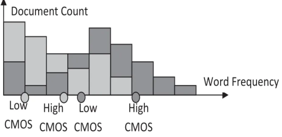
Each class is represented by two BOW vectors, one for each CMQS point used. For each class, we compute the frequency distribution of each word in each document in that class, and generate a frequency histogram for that word. While the traditional BOW approach would then pick the average value of this histogram, our method computes the area of the histogram and determines the
two symmetric QS points. Thus, for example, if we are considering the 27 and 57 QS points of the two distributions, we would pick the word frequencies that encompass the 27 and 57 of the histogram area respectively. The reader must observe the salient characteristic of this strategy: By working with such a methodology, for each word in the BOW, we represent the class by two of its non-central cases, rather than its average/median sample. This renders the strategy to be “Anti”-Bayesian!
For further clarity, we refer the reader to Figure 1. For any word, the histograms of the two classes are depicted in light grey for the lower class, and in dark grey for the higher class. The QS-based features for the classes are then extracted from the histograms as clarified in the figure.
Word Frequency
Document Count
Low
CMOS
Low
CMOS
w
OS
L
CM
High
CMOS
High
CMOS
Figure 1: Example of the QS-based features extracted from the histogram of a lower class (light grey) and of a higher class (dark grey), and the corresponding lower and higher CMQS points of each class.
3.3.2 “Anti”-Bayesian TC Solution: The Multi-Class TC Classifier
Let us assume that the PR problem involvesCclasses. Since the “Anti”-Bayesian technique has been extensively studied for two-class problems, our newly-proposed multi-class TC classifier operates by invoking a sequence of C−1 pairwise classifiers. More explicitly, whenever a document for testing is presented, the system invokes a classifier that involves a pair of classes from which it determines a winning class. This winning class is then compared to another class until all the classes have been considered. The final winning class is the overall best and is the one to which the testing document is assigned.
3.3.3 “Anti”-Bayesian TC Solution: Testing
To classify an unknown document, we compute the cosine similarity between it and the features representing pairs of classes. This is done as follows: For each word, we mark one of the two groups as the high-group and the other as the low-group based on the word’s frequency in the documents
of each class, and we take the high CMQS point of the low-group and the low CMQS point of the high-group, as illustrated in Figure 1. We build the two class vectors from these CMQS points, and we compute the cosine similarity between the document to classify each class vector using Eq. (1).
sim(c, d) = W−1 i=0 wicwid W−1 i=0 wic2 W−1 i=0 wid2 . (1)
The most similar class is retained and the least similar one is discarded and replaced by one of the other classes to be considered, and the test is run again, until all the classes have been exhausted. The final class will be the most similar one, and the one that the document is classified into.
4
Experimental Set-Up
4.1 The Data Sets
For our experiments, we used the 20-Newsgroups corpus, a standard corpus in the literature per-taining to Natural Language Processing. This corpus contains 1,000 postings collected from the 20 different Usenet groups, each associated with a distinct topic, as listed in Table 1. We preprocessed each posting by removing header data (for example, “from”, “subject”, “date”, etc.) and lines quoted from previous messages being responded to (which start with a ‘>’ character), performing stop-word removal and word stemming, and deleting the postings that became empty of text after these preprocessing phases.
Table 1: The topics from the “20-Newsgroups” used in the experiments.
comp.graphics alt.atheism sci.crypt misc.forsale
comp.sys.mac.hardware talk.religion.misc sci.electronics rec.autos
comp.windows.x talk.politics.guns sci.med rec.motorcycles
comp.os.ms-windows.misc talk.politics.mideast sci.space rec.sport.hockey comp.sys.ibm.pc.hardware talk.politics.misc soc.religion.christian rec.sport.baseball
In every independent run, we randomly selected 70% of the postings of each newsgroup to be used as training data, and retained the remaining 30% as testing data.
4.2 The Histograms/Features Used
We first describe the process involved in the construction of the histograms and the extraction of the Quantile-based features.
Each document in the 20-Newsgroups dataset was preprocessed by word stemming using the Porter Stemmer algorithm and by a stopword removal phase. It was then converted to a BOW representation. The documents were then randomly assigned into training or testing sets.
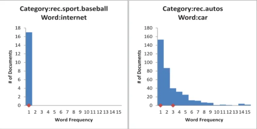
The word-based histograms (please see Figure 2) were then computed for each word in each category by tallying the observed frequencies for that word in each training document in that category, where the area of each histogram was the total sum of all the columns. The CMQS points were determined as those points where the cumulative sum of each column was equal to the CMQS moments when normalized with the total area. For further clarification, we present an example of two histograms9 in Figure 2 below. The13 and 23 QS points of each histogram are marked along their horizontal axes. In this case, the markings represent the word frequencies that encompass the 13 and 23 areas of the histograms respectively. The histogram on the left depicts a less significant word for its category while the histogram on the right depicts a more significant word for its category. Note that in both histograms the first CMQS point is located at unity. To help clarify the figure, we mention that for the word “internet” in “rec.sport.baseball”, both the CMQS points lie at unity - i.e., they are on top of each other.
0 2 4 6 8 10 12 14 16 18 1 2 3 4 5 6 7 8 9 10 11 12 13 14 15 # o f Do cu m en ts Word Frequency Category:rec.sport.baseball Word:internet 0 20 40 60 80 100 120 140 160 180 1 2 3 4 5 6 7 8 9 10 11 12 13 14 15 # o f Do cu m en ts Word Frequency Category:rec.autos Word:car
Figure 2: The histograms and the 13 and 23 QS points for the two words “internet ” and “car” from the categories “rec.sport.baseball” and “rec.autos”.
4.3 The Benchmarks Used
We have developed three benchmarks for our system: A BOW classifier which involved the TFs and invoked the cosine similarity measure given by Eq. (1), a BOW classifier with the TFIDF features, and a Na¨ıve-Bayes’ classifier.
To understand how they all fit together, we define the Term Frequency (TF) of a word (synony-mous with “term”) tin a documentdas Freq(t, d), and for each document this is calculated as the
9The documents used in this test were very short, which explains why the histograms are heavily skewed in favour
frequency count of the term in the document. This is, quite simply, given by Eq. (2):
TF(t, d) = Freq(t, d), (2)
where Freq(t, d) is the number of times that the termt occurs in the documentd.
The BOW classifier computes an average word/term vector wc for each class c, which contains the average occurrence frequency of each of the W terms in that class (i.e., wtc). It computes this by adding together the frequency count of each term as it occurs in each document of a class, and by then dividing the total by the number of documents in the class (Nc), as per Eq. (3).
wtc= 1 Nc Nc d=1 TF(t, d). (3)
The quantity wtc defined in Eq. (3) can also be seen to be the TF value as calculated perclass
instead of per document. Thus, to be explicit:
TF(t, c) =wtc, (4)
where wtc is specified in Eq. (3).
Classifying a test document, d, is done by computing the cosine similarity of that test doc-ument’s TF vector (which will likewise contain the occurrence frequency of each word in that document, TF(t, d)) with the TF for each each class, TF(t, c), as per Eq. (1), and assigning the document to the most similar class.
The IDF, or Inverse Document Frequency, is the inverse ratio of the number of term vectors in the training corpus containing a given word. Specifically, if Nt is the number of classes in the training corpus containing a given term t, and C is the total number of classes in the corpus, the IDF(t) is given as in Eq. (5):
IDF(t) = log10 C
Nt. (5)
Combining the above, we get the TFIDF valueper document as the quantity calculated by:
TFIDF(t, d) = TF(t, d)×IDF(t), (6)
where TF(t, d) is given by Eq. (2).
Analogously, the TFIDF valueper class is the quantity calculated as:
TFIDF(t, c) = TF(t, c)×IDF(t), (7)
The Na¨ıve-Bayes’ classifier selects the class c∗ which is most probable one given the observed document, following Eq. (8). This is based on the prior probability of the class being independent of any other information, P(c), multiplied by the probability of observing each individual word of the document t in the class, P(t|c). This probability is computed as the frequency count of each word in the class divided by its frequency count in the entire corpus of N documents, as in Eq. (9). Finally, in order to avoid multiplications by zero in the case of a term that was never before seen in a class, we set the minimal value for P(t|c) to be one thousandth of the minimum probability that was actually observed.
c∗= arg max c P(c) t∈c P(t|c) . (8)
Also, since every class in the corpus had an equal number of documents and equal likelihood, the term for the a priori probability P(c) in Eq. (8) was set to be always equal to 1/20, and was thus ignored. P(wi|c) = Nc d=1 wid N d=1 wid . (9)
4.4 The Testing and Accuracy Metrics Used
4.4.1 The Metrics Used
In every testing case, we used the respective data to train and test our classifier and each of the three benchmark schemes. For each newsgroup i, we counted the numberT Pi of postings correctly identified by a classifier as belonging to that group, the number F Ni of postings that should have belonged in that group but were misidentified as belonging to another group, and the numberF Pi
of postings that belonged to other groups but were misidentified as belonging to this one. The Precision Pi is the proportion of postings assigned in group ithat are correctly identified, and the Recall Ri is the proportion of postings belonging in the group that were correctly recognized, and are given by Eq. (10) and Eq. (11) respectively. The F score is an average of these two metrics for each group, and the macro-F1 is the average of the F scores over the all groups, and these are given in Eq. (12) and Eq. (13) respectively.
Pi = T Pi
T Pi+F Pi (10)
Ri= T Pi
Fi = 2PiRi Pi+Ri (12) macro-F1 = 1 20 20 i=1 Fi (13)
4.4.2 Correlation between the Classifiers
Since the features and methods used in the classification are rather distinct, it would be a remarkable discovery if we could confirm that the results between the various classifiers are not correlated. In this regard, it is crucial to understand what the term “correlation” actually means. Formalized rigorously, the statistical correlation between two classifiers, X and Y would be defined as in Eq. (14) below: ClassifierCorrX,Y = N−1 i=1 xi−x¯ yi−y¯ N σXσY , (14)
where X and Y are the classifiers being compared, xi and yi are ‘0’ or ‘1’, and are the assigned values for incorrect and correct classifications of document iby X and Y respectively, ¯x and ¯y are the average performances of X and Y over all the documents,N is the number of documents, and
σX and σY are the standard deviations of the performances ofX and Y respectively.
However, on a deeper examination, one would observe that while Eq. (14) yields thestatistical
correlation, it is only suited to classifiers that yield accuracies within the interval [0,1]. It is, thus, not the best equation to compare the classifiers that we are dealing with. Rather, since the classifiers themselves yield binary results (‘0’ or ‘1’ for incorrect or correct classifications), it is more appropriate to compare classifiers Xand Y by the “number” of times they yieldidenticaldecisions. In other words, a more suitable metric for evaluating how any two classifiersX andY yield identical results is given by Eq. (15) below:
ClassifierSimX,Y = P osXP osY +N egXN egY
P osXP osY +P osXN egY +N egXP osY +N egXN egY , (15)
where P osXP osY and N egXN egY are the count of cases where the classifiers X and Y both return identical decisions ‘1’ or ‘0’ respectively, and where ‘0’ and ‘1’ represent the events of a classifier classifying a document incorrectly or correctly respectively. Analogously, P osXN egY and
N egXP osY are the counts of cases whereXreturns ‘1’ andY returns ‘0’ and vice-versa respectively. The reader should observe that strictly speaking, this metric would not yield a statistical correlation between the classifiers X and Y, but rather a statistical measure of their relative similarities. However, in the interest of maintaining a relatively acceptable terminology (and since we have
previously used the term “similarity” to imply the similarity between documents and classes as opposed to the similarity between theclassifiers), we shall informally refer to this classifier similarity as their mutual correlation, because, it does, in one sense, inform us about how correlated the decision made by classifier X is to the decision made by classifierY.
5
Experimental Results
In this section, we shall present the results that we have obtained by testing our “Anti”-Bayesian (indicated, in the interest of brevity, by AB in the tables and figures) methodology against the benchmark classifiers described above. There are, indeed, two sets of results that are available: The first involves the case when the “Anti”-Bayesian scheme uses only the TF criteria, and this is done in Section 5.1. This is followed by the results when the “Anti”-Bayesian paradigm invokes the TFIDF criteria, i.e., when the lengths of the documents are also involved in characterizing the features. These results are presented in Section 5.2. A comparison and the correlation between these two sets of “Anti”-Bayesian schemes themselves is finally given in Section 5.3.
5.1 The Results Obtained: “Anti”-Bayesian TF Scheme
The experimental results that we have obtained for the “Anti”-Bayesian scheme that used only the TF criteria are briefly described below. We performed 100 tests, each one using a different random 70%/30% split of training and testing documents. We then evaluated the results of each classifier by computing the Precision, Recall, andF-score of each newsgroup, whence we computed
the macro-F1 value for each classifier over the 20-Newsgroups. The average results we obtained,
over all 100 tests, are summarized in Table 2.
We summarize the results that we have obtained:
1. The results show that for half of the CMQS pairs, the “Anti”-Bayesian classifier performed as well as and sometimes even better than the traditional BOW classifier. For example, while the BOW had a Macro-F1 score of 0.604, the corresponding index for the CQMS pairs
13,23, was remarkably higher, i.e., 0.662. Further, the macro-F1 score indices for 25,35,
3
7,47and49,59were consistently higher – 0.700, 0.710 and 0.713 respectively. This, in itself,
is quite remarkable, since our methodology is reversed to the traditional ones. This is also quite fascinating, given that it uses points distant from the mean (i.e., moving towards the extremities of the distributions) rather than the averages that are traditionally considered.
2. While the results obtained for extreme CMQS points very distant from the mean were not so impressive10, the corresponding results for other non-central QS pairs were very encouraging.
Table 2: The macro-F1 score results for the 100 classifications attempted and for the different methods. In the case of the “Anti”-Bayesian scheme, the method used the TF features.
Classifier CMQS Points macro-F1 Score
“Anti”-Bayesian 1/2, 1/2 0.709 1/3, 2/3 0.662 1/4, 3/4 0.561 1/5, 4/5 0.465 2/5, 3/5 0.700 1/6, 5/6 0.389 1/7, 6/7 0.339 2/7, 5/7 0.611 3/7, 4/7 0.710 1/8, 7/8 0.288 3/8, 5/8 0.686 1/9, 8/9 0.264 2/9, 7/9 0.515 4/9, 5/9 0.713 1/10, 9/10 0.243 3/10, 7/10 0.631 BOW 0.604 BOW-TFIDF 0.769 Na¨ıve-Bayes 0.780
For example, the corresponding index for the CQMS pairs 27,57 was much higher than the BOW index, i.e., 0.611.
3. The results of the BOW and the “Anti”-Bayesian classifier were always less than what was obtained by the BOW-TFIDF and the Na¨ıve-Bayes’ classifier. This result is actually easily explained, because while all the classifiers compare vectors using cosine similarities, the BOW-TFIDF uses the more-informed document-weighted features. We shall presently show that if we use corresponding TFIDF-based features (that are more suitable for such text-based classifiers) with an “Anti”-Bayesian paradigm , we can obtain a comparable accuracy. That being said, the question of determining the best metric to be used for an “Anti”-Bayesian classifier in this syntactic space is currently unresolved.
Since the features/methodology used by the “Anti”-Bayesian classifier are different than those used by the traditional classifiers, it follows that they would perform differently, and either correctly or incorrectly classify different documents, as seen from a correlation-based analysis below. To verify this, we computed the correlation, as defined by Eq. (15), between the results of the “Anti”-Bayesian classifier in each of our 100 tests and the three benchmarks classifiers. Observe that a correlation near to unity would indicate that the corresponding two classifiers make identical decisions on the
criteria (instead of merely the TF criteria), we hypothesize that this poor behavior is probably due to noise from non-significant words that is somehow amplified in the extreme CMQS points. But this issue is still unresolved.
same documents – either correctly and incorrectly, while a correlation around ‘0’ would indicate that their classification results are unrelated. The average correlation scores for the classifiers over all 100 tests are given in Table 3. The following points are noteworthy:
1. “Anti”-Bayesian classifiers that use CMQS points that are farther from the mean or median of the distributions show a lower correlation with the 12,12 “Anti”-Bayesian classifier. This is, actually, quite remarkable, considering that they sometimes give comparable accuracies even though they use completely different features. It also implies that two classifiers built from the same data and statistics but that utilize different CMQS points will have different behaviours and also yield different results. This is all the more interesting since, from Table 2, we can see that these classifiers will, in many cases, have similar macro-F1 scores. This indicates that a fusion classifier that combines the information from multiple CMQS points could outperform any single classifier, and be built without requiring any additional data or tools from that classifier.
Table 3: The correlation between the different classifiers for the 100 classifications achieved. In the case of the “Anti”-Bayesian scheme, the method used the TF features.
Classifier CMQS Points AB at (1/2, 1/2) BOW BOW with TFIDF Na¨ıve-Bayes
“Anti”-Bayesian 1/2, 1/2 1.000 0.648 0.759 0.810 1/3, 2/3 0.845 0.642 0.722 0.772 1/4, 3/4 0.738 0.625 0.646 0.676 1/5, 4/5 0.646 0.595 0.570 0.589 2/5, 3/5 0.902 0.643 0.747 0.806 1/6, 5/6 0.579 0.568 0.514 0.526 1/7, 6/7 0.537 0.549 0.478 0.487 2/7, 5/7 0.790 0.635 0.684 0.723 3/7, 4/7 0.925 0.643 0.755 0.816 1/8, 7/8 0.496 0.527 0.439 0.445 3/8, 5/8 0.882 0.642 0.738 0.794 1/9, 8/9 0.478 0.517 0.423 0.429 2/9, 7/9 0.695 0.613 0.612 0.637 4/9, 5/9 0.938 0.643 0.757 0.818 1/10, 9/10 0.462 0.509 0.408 0.414 3/10, 7/10 0.811 0.638 0.699 0.743 BOW 0.648 1.000 0.714 0.654 BOW-TFIDF 0.759 0.714 1.000 0.800 Na¨ıve-Bayes 0.810 0.654 0.800 1.000
2. It is surprising to see that the “Anti”-Bayesian classifiers, almost consistently, have higher correlations with the two benchmarks that performed better than it. Indeed, the BOW-TFIDF classifier and the Na¨ıve-Bayes’ classifier show much larger correlations than the BOW classifier. In fact, the correlation between our “Anti”-Bayesian classifier and the BOW classifier is, almost always, the lowest of all the pairs, indicating that they generate the most different
classification results!
3. Figure 3 displays the plots of the correlation between the different classifiers for the 100 classifications achieved, where in the case of the “Anti”-Bayesian scheme, the method used the TF features. The reader should observe the uncorrelated nature of the classifiers when the CMQS points are non-central, and the fact that this correlation increases as the feature points become closer to the mean or median.
0.00 0.10 0.20 0.30 0.40 0.50 0.60 0.70 0.80 0.90 1.00 1/10 1/5 3/10 2/5 1/2 Pe rcentile Anti-Bayesian CMQS Points AB Macro-F1 Score Correlation of AB and AB at (1/2, 1/2) Correlation of AB and BOW Correlation of AB and BOW with TF-IDF Correlation of AB and Naïve-Bayes'
Figure 3: Plots of the correlation between the different classifiers for the 100 classifications achieved. In the case of the “Anti”-Bayesian scheme, the method used the TF features.
5.2 The Results Obtained: “Anti”-Bayesian TFIDF Scheme
The results of the “Anti”-Bayesian scheme when it involves TFIDF features are shown in Table 4. In this case, the TF is calculated per document as per Eq. (6) for the test document, and as per Eq. (7) for each of the classes it is tested against. From this table we can glean the following results:
1. The results show that for all CMQS pairs, the “Anti”-Bayesian classifier performed much better than the traditional BOW classifier. For example, while the BOW had a macro-F1
score of 0.604, the corresponding index for the CQMS pairs13,23, was significantly higher, i.e., 0.747. Further, themacro-F1score indices for14,34,37,47and49,59were consistently higher – 0.746, 0.744 and 0.744 respectively. This demonstrates the validity of our counter-intuitive paradigm – that we can truly get a remarkable accuracy even though we are characterizing the documents by the syntactic features of the points quite distant from the mean and more towards the extremities of the distributions.
2. In all the cases, the values of the Macro-F1 index was only slightly less than the indices obtained using the BOW-TFIDF and the Na¨ıve-Bayes approaches.
Table 4: The macro-F1 score results for the 100 classifications attempted and for the different methods. In the case of the “Anti”-Bayesian scheme, the method used the TFIDF features.
Classifier CMQS Points macro-F1 Score
“Anti”-Bayesian 1/2, 1/2 0.742 1/3, 2/3 0.747 1/4, 3/4 0.746 1/5, 4/5 0.742 2/5, 3/5 0.745 1/6, 5/6 0.736 1/7, 6/7 0.729 2/7, 5/7 0.747 3/7, 4/7 0.744 1/8, 7/8 0.720 3/8, 5/8 0.746 1/9, 8/9 0.712 2/9, 7/9 0.745 4/9, 5/9 0.744 1/10, 9/10 0.705 3/10, 7/10 0.748 BOW 0.604 BOW-TFIDF 0.769 Na¨ıve-Bayes 0.780
Since the features/methodology used by the “Anti”-Bayesian classifier are different than those used by the traditional classifiers, it is again advantageous to embark on a correlation-based analysis. To achieve this, we have again computed the correlation, as defined by Eq. (15) between the results of the “Anti”-Bayesian classifier (using the TFIDF criteria) in each of our 100 tests, and the three benchmarks classifiers. As before, a correlation near to unity would indicate that the corresponding two classifiers make identical decisions on the same documents – either correctly and incorrectly, while a correlation around ‘0’ would indicate that their classification results are unrelated. The average correlation scores for the classifiers over all 100 tests are given in Table 5.
From the table, we observe the following rather remarkable points:
1. The first result that we can infer is that just as in the case when we used the TF features, the “Anti”-Bayesian classifier using the TFIDF criteria, when it works with CMQS points that are not near the mean or the median, has lower correlation than the benchmark classifiers that works with CMQS points that are near the mean or median, Indeed, they sometimes give comparable accuracies even though they use completely different features.
2. Again, the “Anti”-Bayesian classifier actually has the highest correlation in its results with the two benchmarks that performed better than it. This means that although the classification algorithm is similar to a BOW classifier, its results are more closely aligned to those of the more-informed TFIDF and NB classifiers.
Table 5: The correlation between the different classifiers for the 100 classifications achieved. In the case of the “Anti”-Bayesian scheme, the method used the TFIDF features.
Classifier CMQS Points AB at (1/2, 1/2) BOW BOW with TFIDF Na¨ıve-Bayes
“Anti”-Bayesian 1/2, 1/2 1.000 0.636 0.780 0.832 1/3, 2/3 0.946 0.635 0.784 0.836 1/4, 3/4 0.928 0.635 0.786 0.831 1/5, 4/5 0.913 0.634 0.785 0.824 2/5, 3/5 0.960 0.635 0.780 0.835 1/6, 5/6 0.898 0.632 0.781 0.817 1/7, 6/7 0.887 0.631 0.779 0.811 2/7, 5/7 0.936 0.635 0.785 0.833 3/7, 4/7 0.968 0.635 0.779 0.834 1/8, 7/8 0.873 0.626 0.771 0.800 3/8, 5/8 0.954 0.635 0.781 0.835 1/9, 8/9 0.862 0.625 0.768 0.794 2/9, 7/9 0.920 0.635 0.786 0.829 4/9, 5/9 0.974 0.636 0.779 0.834 1/10, 9/10 0.853 0.624 0.764 0.788 3/10, 7/10 0.939 0.636 0.785 0.834 BOW 0.636 1.000 0.714 0.654 BOW-TFIDF 0.780 0.714 1.000 0.800 Na¨ıve-Bayes 0.832 0.654 0.800 1.000
3. Even when the “Anti”-Bayesian classifier used points very distant from the mean (for example,
1
10,109 ), the correlation was as high as 0.764. This means that there were more than 76%
of the cases when they both used completely different classifying criteria and yet produced similar results.
4. Figure 4 displays the plots of the correlation between the different classifiers for the 100 classifications achieved, where in the case of the “Anti”-Bayesian scheme, the method used the TFIDF features. The reader should observe the uncorrelated nature of the classifiers when the CMQS points are non-central. This correlation increases as the feature points become closer to the mean or median.
5.3 Correlation between “Anti”-Bayesian TF versus TFIDF Schemes
The correlated/uncorrelated nature of the “Anti”-Bayesian TF and TFIDF schemes with the other methods was explained in the earlier sections. It would be educative to examine how uncorrelated the “Anti”-Bayesian TF and the “Anti”-Bayesian TFIDF schemes are between themselves. In other words, even though their accuracies may be comparable, it would be good to examine if the two “Anti”-Bayesian classifiers are relatively uncorrelated in and of themselves. Thus, if a particular pair of CMQS points yielded distinct classification decisions using the two schemes, and if they, all the same, yielded comparable accuracies, the potential of the paradigm is shown to be significantly
0.00 0.10 0.20 0.30 0.40 0.50 0.60 0.70 0.80 0.90 1.00 1/10 1/5 3/10 2/5 1/2 Pe rcentile Anti-Bayesian CMQS Points AB Macro-F1 Score Correlation of AB and AB at (1/2, 1/2) Correlation of AB and BOW Correlation of AB and BOW with TF-IDF Correlation of AB and Naïve-Bayes'
Figure 4: Plots of the correlation between the different classifiers for the 100 classifications achieved. In the case of the “Anti”-Bayesian scheme, the method used the TFIDF features.
more. This is precisely what we embark on achieving now – i.e., examining the correlation (or lack thereof) of the “Anti”-Bayesian TF and TFIDF schemes.
Table 6 reports the correlation, as defined by Eq. (15) between the results of the “Anti”-Bayesian classifier TF and TFIDF criteria in each of our 100 tests. The table also include the corresponding Macro-F1 scores. Again, a correlation near to unity would indicate that the two classifiers make identical decisions on the same documents – either correctly and incorrectly, while a correlation around ‘0’ would indicate that their classification results are unrelated. The results tabulated in Table 6 are also depicted graphically in Figure 5 whence the trends in the correlation with the increasing values of the CMQS points is clear.
0.00 0.10 0.20 0.30 0.40 0.50 0.60 0.70 0.80 0.90 1.00 1/10 3/20 1/5 1/4 3/10 7/20 2/5 9/20 1/2 Pe rce nt ile Anti-Bayesian CMQS Points AB Macro-F1 Score AB TFIDF Macro-F1 Score Correlation of AB and AB TFIDF
Figure 5: The correlation between the two “Anti”-Bayesian classifiers for the 100 classifications when they utilized the TF and the TFIDF features respectively.
Table 6: The correlation between the two “Anti”-Bayesian classifiers for the 100 classifications when they utilized the TF and the TFIDF features respectively.
Classifier CMQS Points AB Macro-F1 AB TFIDF Macro-F1 Correlation of AB and AB TFIDF “Anti”-Bayesian 1/2, 1/2 0.709 0.742 0.842 1/3, 2/3 0.662 0.747 0.792 1/4, 3/4 0.561 0.746 0.699 1/5, 4/5 0.465 0.742 0.616 2/5, 3/5 0.700 0.745 0.833 1/6, 5/6 0.389 0.736 0.557 1/7, 6/7 0.339 0.729 0.523 2/7, 5/7 0.611 0.747 0.745 3/7, 4/7 0.710 0.744 0.845 1/8, 7/8 0.288 0.720 0.493 3/8, 5/8 0.686 0.746 0.819 1/9, 8/9 0.264 0.712 0.481 2/9, 7/9 0.515 0.745 0.659 4/9, 5/9 0.713 0.744 0.848 1/10, 9/10 0.243 0.705 0.472 3/10, 7/10 0.631 0.748 0.762
1. When the CMQS points are close to the mean or median, the correlation is quite high (for example, 0.842). This is not surprising at all, since in such cases, the “Anti”-Bayesian classifier reduces to become a Bayesian classifier.
2. When the CMQS points are far from the mean or median, the correlation is quite high (for example, 0.659 for the CMQS points 29,79). This is quite surprising because although both schemes are “Anti”-Bayesian in their philosophy, the lengths of the documents play a part in determining the decisions that they individually make because the IDF values account for document lengths.
3. From the values of the associated Macro-F1 scores, we see that a lower correlation between these two classifiers is directly related to their difference in accuracy. This means that when the accuracies of the two classifiers are lower, each of them is classifying the documents on distinct criteria – which is far from being obvious.
This naturally leads us to our final section which deals with how we can fuse the results of the various classifiers.
5.3.1 On Utilizing Classifier Fusion
This section briefly touches on possible exploratory work, where we consider how the various clas-sifiers can be “fused”.
Combined with the aforementioned fact that they use a completely different set of features for classification, and that they are the two simplest of the five classifiers we considered, let us consider how the BOW and “Anti”-Bayesian scheme using the TF features can be fused. Indeed, it would be interesting to see how they could be combined by incorporating a relatively simple data fusion technique. As a preliminaryprima facieexperiment in that direction, we combined the classification of the BOW classifier and our “Anti”-Bayes classifier (using the TF criteria) in each of our 100 experiments. Since each classifiers measures the similarity between a document and the classes’ feature vectors and then picks the maximum, we performed this combination simply by comparing the winning (for example, the highest) class similarity value returned by each of the two classifiers and picking the maximum one. We found that this classifier obtains an average macro-F1 score of 0.674, only marginally better than the 0.671 macro-F1 score of the best “Anti”-Bayes classifier in our tests. Upon further examination, we find that this is due to the fact that the similarity values generated by the “Anti”-Bayes classifier are on average three times higher than those generated by the BOW classifier. Consequently, the “Anti”-Bayes classification is the one picked in almost all cases! However, the few cases where the BOW classifier’s similarity score beats that of the “Anti”-Bayes classifier are also cases where the BOW correctly classified documents that the “Anti”-Bayes classifier missed, leading to the small improvement observed in the results. Moreover, our data shows that there are more than 1,000 documents (over 12% of the test corpus) that the BOW classifier correctly classifies with a similarity that is less than that of the “Anti”-Bayesian’s erroneous classification.
There is thus clear room for improvements in the final classification, and the main challenge for future research will involve developing a fair weighting scheme between the two classifiers in order to compensate for the lower similarity scores of the BOW classifier, without misclassifying the over 1,500 test documents that the “Anti”-Bayesian classifier recognizes correctly but that the BOW misclassifies.
Indeed, the potential of designing fused classifiers involving the BOW, the BOW-TFIDF, the Na¨ıve Bayes, the “Anti”-Bayesian using the TF criteria, and the “Anti”-Bayesian that uses the TDIDF criteria, is extremely great considering their relative accuracies and correlations.
6
Conclusions
In this paper we have considered the problem of Text Classification (TC), which is a problem that has been studied for decades. From the perspective of classification, problems in TC are particularly fascinating because while the feature extraction process involves syntactic or semantic
indicators, the classification uses the principles of statistical Pattern Recognition (PR). The state-of-the-art in TC uses these statistical features in conjunction with the well-established methods such
as the Bayesian, the Na¨ıve Bayesian, the SVM etc. Recent research has advanced the field of PR by working with the Quantile Statistics (QS) of the features. The resultant scheme called Classification by Moments of Quantile Statistics (CMQS) is essentially “Anti”-Bayesian in its modus operandus, and advantageously works with information latent in “outliers” (i.e., those distant from the mean) of the distributions. Our goal in this paper was to demonstrate the power and potential of CMQS to work within thevery high-dimensional TC-related vector spaces and their “non-central” quantiles. To investigate this, we considered the cases when the “Anti”-Bayesian methodology used both the TD and the TFIDF criteria.
Our PR solution for C categories involved C −1 pairwise CMQS classifiers. By a rigorous testing on the well-acclaimed data set involving the 20-Newsgroups corpus, we demonstrated that the CMQS-based TC attains accuracy that is comparable to and sometimes even better than the BOW-based classifier, even though it essentially uses the information found only in the “non-central” quantiles. The accuracies obtained are comparable to those provided by the BOW-TFIDF and the Na¨ıve Bayes classifier too!
Our results also show that the results we have obtained are often uncorrelated with the estab-lished ones, thus yielding the potential of fusing the results of a CMQS-based methodology with those obtained from a more traditional scheme.
References
[1] A. Alahmadi, A. Joorabchi, and A. E. Mahdi. A New Text Representation Scheme Combining Bag-of-Words and Bag-of-Concepts Approaches for Automatic Text Classification. Proceedings
of the 7th IEEE GCC Conference and Exhibition, Doha, Qatar, November 2014, pp. 108–113.
[2] F. Debole and F. Sebastiani. Supervised Term Weighting for Automated Text Categorization.
Proceedings of the 18th ACM Symposium on Applied Computing, Melbourne USA, 784–788,
March 2003, pp. 784-788.
[3] R. O. Duda and P. E. Hart and D. G. Stork Pattern Classification. A Wiley Interscience Publication, 2006.
[4] J. Dumoulin. Smoothing of n-gram Language Models of Human Chats. Proceedings of the Joint 6th International Conference on Soft Computing and Intelligent Systems (SCIS) and
13th International Symposium on Advanced Intelligent Systems (ISIS), Kobe, Japan, November
2012, pp. 1-4.
[5] L. Lu and Y.-S. Liu. Research of English Text Classification Methods based on Semantic
Mean-ing. Proceedings of the ITI 3rd International Conference on Information and Communications
[6] R. E. Madsen, S. Sigurdsson, L. K. Hansen and J. Larsen. Pruning the Vocabulary for Better Context Recognition.Proceedings of the 17th International Conference on Pattern Recognition, Cambridge, UK, Vol. 2, August 2004, pp. 483-488.
[7] R. Menon, S. S. Keerthi, H. T. Loh and A. C. Brombacher. On the Effectiveness of Latent Semantic Analysis for the Categorization of Call Centre Records. Proceedings of the IEEE
International Engineering Management Conference, Singapore, Vol. 2, October 2004, pp. 545–
550.
[8] Y. Ning, T. Zhu and Y. Wang. Affective-word based Chinese Text Sentiment Classification.
Proceedings of the 5th International Conference on Pervasive Computing and Applications
(ICPCA), Maribor, Slovenia, December 2010, pp. 111-115.
[9] B. J. Oommen and A. Thomas. Optimal Order Statistics-based “Anti-Bayesian” Parametric Pattern Classification for the Exponential Family. Pattern Recognition, Vol. 47, 2014, pp. 40-55.
[10] S. Ouamour and H. Sayoud. Authorship Attribution of Ancient Texts Written by Ten Arabic Travelers using Character N-Grams. Proceedings of the 2013 International Conference on
Computer, Information and Telecommunication Systems (CITS), Piraeus-Athens, Greece, May
2013, pp. 1-5.
[11] G. Qiang. An Effective Algorithm for Improving the Performance of Na¨ıve Bayes for Text Classification. Proceedings of the Second International Conference on Computer Research and
Development, Kuala Lumpur, Malaysia, May 2010, pp. 699-701.
[12] G. Salton and M. McGill. Introduction to Modern Information Retrieval. New York: Mc-Graw Hill Book Company. 1983.
[13] G. Salton, A. Wong, and C. S. Yang. A Vector Space Model for Automatic Indexing. Comm.
of the ACM, Vol. 18, 1975, pp.613-620.
[14] G. Salton, C. S. Yang, and C. Yu. A theory of term importance in automatic text analysis.
Technical Report, Ithaca, NY, USA, 1974.
[15] G. Salton, C. S. Yang, and C. Yu. Term weighting approaches in automatic text retrieval.
Technical Report, Ithaca, NY, USA, 1987.
[16] F. Sebastiani. Machine Learning in Automated Text Categorization. ACM Computing Surveys, 2002, Vol. 34, pp. 1-47.
[17] A. Thomas and B. J. Oommen. The Fundamental Theory of Optimal “Anti-Bayesian” Para-metric Pattern Classification Using Order Statistics Criteria. Pattern Recognition, Vol. 46, 2013, pp. 376-388.
[18] A. Thomas and B. J. Oommen. Order Statistics-based Parametric Classification for Multi-dimensional Distributions. Pattern Recognition, Vol. 46, 2013, pp. 3472-3482.
[19] A. Thomas and B. J. Oommen. Corrigendum to Three Papers that deal with “Anti”-Bayesian Pattern Recognition. Pattern Recognition, Vol. 47, 2014, pp. 2301-2302.
[20] A. Thomas and B. J. Oommen. A Novel Border Identification Algorithm Based on an “Anti-Bayesian” Paradigm.Proceedings of CAIP’13, the 2013 International Conference on Computer
Analysis of Images and Patterns, York, UK, August, 2013, pp. 196-203.
[21] A. Thomas and B. J. Oommen. Ultimate Order Statistics-based Prototype Reduction Schemes. Proceedings of AI’13, the 2013 Australasian Joint Conference on Artificial
Intel-ligence, Dunedin, New Zealand, December 2013, pp. 421-433.
[22] G. Wu and K. Liu. Research on Text Classification Algorithm by Combining Statistical and Ontology Methods. Proceedings of the International Conference on Computational Intelligence