Technical University of Madrid
Master Thesis
University Master in artificial intelligence
Learning Bayesian networks
from data by the incremental
compilation of new network
polynomials
Author:
Marco A. Benjumeda Barquita
Supervisors:
Concha Bielza Lozoya and Pedro Larrañaga Múgica
Los modelos probabilísticos gráficos son un importante campo de investigación en inteligencia artificial hoy en día. El alcance de este trabajo comprende el estudio de modelos probabilísticos gráficos dedicados a la representación de distribuciones prob-abilísticas discretas. Dos de las mayores líneas de investigación relacionadas con esta área se centran en la aplicación de inferencia sobre modelos probabilísticos gráficos y en el aprendizaje de modelos probabilísticos gráficos a partir de datos. Tradicional-mente, el proceso de inferencia y el proceso de aprendizaje han sido tratados por separado, pero dado que la estructura de los modelos aprendidos marca la comple-jidad de inferencia, este tipo de estrategias produce en muchas ocasiones modelos muy ineficientes. Con el fin de obtener modelos más ligeros, en esta tesis de fin de máster se propone un nuevo modelo para la representación de polinomios de red, a la que llamamos árboles polinómicos. Los árboles polinómicos son una representación complementaria de las redes Bayesianas que permite una evaluación eficiente de la complejidad de inferencia y proporciona un marco dedicado a la inferencia exacta. También proponemos un conjunto de métodos dedicados a la compilación incremen-tal de árboles polinómicos y un algoritmo para el aprendizaje de árboles polinómicos a partir datos, que utiliza un método voraz de búsqueda y puntuación que incluye la complejidad de inferencia como una penalización en la función de puntuación.
Probabilistic graphical models are a huge research field in artificial intelligence nowa-days. The scope of this work is the study of directed graphical models for the representation of discrete distributions. Two of the main research topics related to this area focus on performing inference over graphical models and on learning graphical models from data. Traditionally, the inference process and the learning process have been treated separately, but given that the learned models structure marks the inference complexity, this kind of strategies will sometimes produce very inefficient models. With the purpose of learning thinner models, in this master the-sis we propose a new model for the representation of network polynomials, which we call polynomial trees. Polynomial trees are a complementary representation for Bayesian networks that allows an efficient evaluation of the inference complexity and provides a framework for exact inference. We also propose a set of methods for the incremental compilation of polynomial trees and an algorithm for learning polynomial trees from data using a greedy score+search method that includes the inference complexity as a penalization in the scoring function.
I want to thank my supervisors Pedro Larrañaga and Concha Bielza for their guid-ance during this master thesis and their confidence in me. I also want to thank my parents for their huge support, that have allowed me to focus on my work without worrying about many other things.
Resumen iii Abstract iv Acknowledgements v Contents vi List of Figures ix List of Tables xi Abbreviations xiii 1 Introduction 1
1.1 Graphical models and Bayesian networks . . . 1
1.2 Motivations . . . 3
1.3 Notation . . . 4
1.4 Structure of the report . . . 4
2 Bayesian Network Models 7 2.1 Bayesian networks . . . 7
2.2 Inference in Bayesian networks. . . 10
2.2.1 Exact inference . . . 11
2.2.2 Approximate inference . . . 13
2.3 Scoring metrics . . . 16
2.3.1 Bayesian metrics . . . 17
2.3.2 Information-theory metrics . . . 19
2.4 Learning the structure of Bayesian networks . . . 21
2.5 Learning thin Bayesian networks . . . 24
3 Network Polynomials 27 3.1 Introduction to network polynomials . . . 27
3.2 Arithmetic circuits . . . 30 vii
3.3 Learning arithmetic circuits . . . 32
3.3.1 Example of split. . . 34
4 Polynomial Trees 37 4.1 Inference in polynomial trees . . . 40
4.1.1 Example. Inference in polynomial trees . . . 43
4.2 Evaluating the complexity of polynomial trees . . . 45
4.2.1 Example. Evaluating the complexity of a polynomial tree . . . 46
4.3 Incremental compilation of polynomial trees . . . 47
4.3.1 Arc addition . . . 48
4.3.2 Arc deletion . . . 53
4.3.3 Arc reversal . . . 54
4.3.4 Polynomial tree optimization . . . 54
4.4 Learning polynomial trees from data . . . 59
4.5 Scoring function . . . 61
4.6 Hill-climbing for polynomial trees . . . 62
5 Experimental Results 67 5.1 Test methodology . . . 68
5.2 Learning Results . . . 69
5.3 Inference Results . . . 71
6 Conclusions and Future Research 83 A Proof of Theorem 1 85 A.1 Properties of the Polynomial trees and notation . . . 85
2.1 Bayesian network Earthquake . . . 8
3.1 Bayesian network BN1. . . 28
3.2 Arithmetic circuit AC1 . . . 31
3.3 Maximizer circuit for AC1 . . . 32
3.4 LearnAC example. BN (top) and AC (bottom) before split.. . . 35
3.5 LearnAC example. BN (top) and AC (bottom) after split. . . 35
4.1 Structure of the Bayesian network BN2. . . 39
4.2 Combination of BN and PT for BN2 (left), and only the PT (right). . 39
4.3 Example. A PT and the parameters of its corresponding BN.. . . 41
4.4 Example of the inference complexity calculation forP . . . 47
4.5 Examples of BN (left) and PT (right) respectively.. . . 49
4.6 Example of arc addition for scenario 1. BN (left) and PT (right). . . 50
4.7 Example of arc addition for scenario 2. BN (left) and PT (right). . . 50
4.8 Example of arc addition for scenario 3. BN (left) and PT (right). . . 51
4.9 Example of an arc deletion. Initial BN (left) and PT (right). . . 54
4.10 Example. Arc reversal. BN and PT respectively. . . 55
4.11 Section of a PT . . . 60 4.12 Step 1 . . . 60 4.13 Step 2 . . . 60 4.14 Step 3 . . . 60 4.15 Step 4a. . . 61 4.16 Step 4b . . . 61
5.1 Inference in ALARM. NMLP for 15 % query variables. . . 74
5.2 Inference in ALARM. NMLP for 15 % evidence variables . . . 74
5.3 Inference in ALARM. MSE for 15 % query variables. . . 75
5.4 Inference in ALARM. MSE for 15 % evidence variables . . . 75
5.5 Inference in HEPAR II. NMLP for 15 % query variables. . . 77
5.6 Inference in HEPAR II. NMLP for 15 % evidence variables . . . 77
5.7 Inference in HEPAR II. MSE for 15 % query variables. . . 78
5.8 Inference in HEPAR II. MSE for 15 % evidence variables . . . 78
5.9 Inference in WIN95PTS. NMLP for 15 % query variables . . . 80
5.10 Inference in WIN95PTS. NMLP for 15 % evidence variables . . . 80
5.11 Inference in WIN95PTS. MSE for 15 % query variables . . . 81 ix
5.12 Inference in WIN95PTS. MSE for 15 % evidence variables . . . 81
A.1 Case 2 of Lemma 1. Before addArc(B,P, Xout, Xin). . . 87
A.2 Case 2 of Lemma 1. After addArc(B,P, Xout, Xin). . . 87
A.3 Case 3 of Lemma 1. Before addArc(B,P, Xout, Xin). . . 89
A.4 Case 3 of Lemma 1. After addArc(B,P, Xout, Xin). . . 89
A.5 Pa. . . 91
A.6 Case 1. . . 91
5.1 Basic properties of the BNs used for the experiments. . . 68
5.2 Sizes of the datasets generated for the experiments. . . 68
5.3 Learning results for ALARM . . . 70
5.4 Learning results for WIN95PTS . . . 70
5.5 Learning results for HEPAR II. . . 70
5.6 Inference in ALARM. 15 % query variables . . . 73
5.7 Inference in ALARM. 15 % evidence variables . . . 73
5.8 Inference in HEPAR II. 15 % query variables . . . 76
5.9 Inference in HEPAR II. 15 % evidence variables . . . 76
5.10 Inference in WIN95PTS. 15 % query variables . . . 79
5.11 Inference in WIN95PTS. 15 % evidence variables . . . 79
AC Arithmetic Circuit
AI Artificial Intelligence
AIC Akaike Information Criterion
BD Bayesian Dirichlet
BIC Bayesian Information Criterion
BN Bayesian Network
CHC Constrained Hill-Climbing
CPD Conditional Probability Distribution
CPT Conditional Probability Table
DAG Direct Acyclic Graph
HC Hill-Climbing
HCPT Hill-Climbing for Polyomial Trees
JT JunctionTree
LL Log-Likelihood
LMM Light Mutual Min
LW Likelihood-Weighting
MCMC Markov Chain Monte Carlo
MDL Minimum Description Length
MMHC Max Min Hill-Climbing
MMPC Max Min Parents andChildren
MP Message Passing
NMLP Normalized Mean Log Probability xiii
NP Network Polynomial
PC Parents andChildren
PLS Probabilistic Logic Sampling
Introduction
1.1
Graphical models and Bayesian networks
During the last decades, there has been an information revolution due to the rise of internet. There are multiple information sources from several fields. Social data can be obtained from the web, from social networks or from official data sources. but there are also huge amounts of data from specific fields. For example, there are mul-tiple datasets related to finance and business, including the stock market data and electronic trading. In science, there are many experimental results published online, there are huge biomedical databases available, and different sources of information for almost every scientific field.
Modelling this data is one of the main topics of artificial intelligence (AI) nowa-days. Models are necessary to reason about the phenomenas collected in the data or to get predictions of the outcome of certain events. The models are also useful to hide the complexity of the real world, and therefore simplify the representation of the problem that we are facing. They can also be applied in situations that are different from the ones where they were learned, so the models should learn the patterns in the data and recognise similar situations.
It is important to mention that most of the domains that we need to deal with in AI involve uncertainty. Probabilistic models are specially interesting, because they handle uncertainty applying the probability theory, that is long-established. These models use probabilities to indicate different degrees of certainty.
Trying to store the full joint probability distribution related to a problem would be intractable, so it is necessary to use a more compact representation of the prob-abilistic models that is useful in practice. The idea is to take advantage of the independences between the variables of the model to avoid unnecessarily big proba-bility tables. Probabilistic graphical models represent the dependences between the variables graphically, usually with a graph structure where the nodes represent the variables of the model and the arcs represent the probabilistic relationships between the variables.
Bayesian networks (BNs) are one of the most popular and successful graphical models. The dependences of the model are represented by directed arcs, so the structure of BNs is a direct acyclic graph (DAG). The name of Bayesian networks comes from the Bayes rule, which they use to compute probabilities. Another in-teresting property of BNs is that they show the relationships between the variables intuitively, so they can be easily consulted or modified by experts. This makes the BN easier to understand for the users.
The next are some of the properties that make BNs so widely used:
• They are probabilistic models. They represent the uncertainty with probabil-ities, which makes the models coherent with the probability theory.
• They are graphical models. They are easily understandable and the relation-ships between the variables are intuitive.
• They are self-explanatory. They do not only give the solutions to problems, but they also provide the justification.
• They favour the representation of causal relationships.
• They can be created by experts or learned from data. Learning BNs from data can be also useful to learn some undiscovered relationships from complex domains.
• There are methods for BNs that can deal with high dimensional domains and large amount of variables.
Although Bayesian networks have many desirable properties, there are also some difficulties related to them that must be considered:
• The complexity of brute force approaches for performing inference in BNs is exponential in the number of variables and it has been proved that both exact
inference (Cooper,1990) and approximate inference (Dagum and Luby,1993) in BNs are NP-Hard.
• Learning BNs from data is an NP-complete problem (Chickering, 1996) and state-of-the-art methods still capture many unnecessary relationships between the variables.
Graphical models, and Bayesian networks in particular, are a huge research field in AI, and there is a great effort and tones of work dedicated to the improvement of the performance and accuracy of the inference and learning procedures.
1.2
Motivations
Traditionally, the inference and learning methods for Bayesian networks have been treated separately. Research works focused on inference methods usually try to improve their efficiency while keeping its faithfulness to the network, while the works focused on learning methods usually try to find the best fitted networks with a limited number of parameters in a tractable time.
The problem with this approach is that the learning process affects dramatically to the efficiency of performing inference in the learned model. The shape of the model is crucial for obtaining networks where the computational complexity of exact inference is tractable. It would be interesting to have algorithms that consider the inference complexity of the learned models in a way that it is possible to learn not only fitted networks, but also models where exact inference is tractable.
The objective of this work is to create a new type of graphical model to complement Bayesian networks during the learning process, so it can be used as an inference complexity indicator, and also provide a framework for exact inference. The idea is that if we can avoid the addition of those arcs that imply a huge increment of the inference complexity and do not improve enough the fitting of the network, we should obtain thinner models without worsening too much their faithfulness, allowing exact inference in many cases.
1.3
Notation
In this section we make a brief review of the notation used in this work.
The notation for mentioning graphical models is a calligraphic capital letter, that can be combined with a sub-index or a super-index. The Bayesian networks are usually represented with a capitalBand the polynomial trees are usually represented with a capital P. An example is the PT P0.
The sets of variables are represented with one or more calligraphic capital letters, that can be combined with a sub-index. An example would be the set of nodes XP.
Each variable is represented with one or more capital letters in italic, that can be combined with a sub-index with lower-case letters or numbers. An example would be the node Xi.
The precedence dependences in the models are represented as follows:
• P a(M, Xi): Parents of the node Xi in modelM.
• Ch(M, Xi): Children of the nodeXi in model M.
• P red(M, Xi): Predecessors of the node Xi in model M.
• Desc(M, Xi): Descendants of the node Xi in modelM.
When knowing which model is M is trivial, sometimes the precedence notation is simplified and M is not mentioned. For example, P a(Xi) could be mentioned
instead of P a(M, Xi).
1.4
Structure of the report
• Chapter 1contains an introduction to the graphical models and the motiva-tions of this work.
• Chapter 2 contains the definition of Bayesian networks (BNs), and reviews some of the most relevant methods for inference and learning in BNs.
• Chapter 3 is an introduction to network polynomials (NPs). It includes the definition of arithmetic circuits (ACs) and reviews some methods for learning ACs from data.
• Chapter 4 contains the definition of the polynomial trees (PTs), the new model proposed for representing network polynomials. It includes the meth-ods proposed for the incremental compilation and optimization of PTs, and a method for learning PTs from data.
• Chapter 5consists of a set of experimental tests over the proposed PT learn-ing algorithm.
• Chapter 6includes the conclusions of this master thesis and discusses about possible future research work related to PTs.
Bayesian Network Models
2.1
Bayesian networks
Bayesian networks are very powerful tools for modelling probability distributions. They belong to the family of probabilistic graphical models, and specifically, each BN represents a probability distribution over a set of variables X ={X1, X2, . . . , Xn}.
A BN encodes the conditional dependences between the variables in X, and it is composed of:
1. Directed acyclic graph: Each node of the graph represents a random variable in X, and each directed arc Xi → Xj represents the conditional dependence
between Xi and Xj.
2. Parameters: Each variableXi ∈ X has a conditional probability distribution P(Xi, P a(Xi)). This probability distributions are called the parameters of
the network. The parameters of the network can be represented in multiple ways. For discrete networks, conditional probability tables (CPTs) are the most common choice. Gaussians (Geiger and Heckerman, 1994; Shachter and Kenley, 1989; Lauritzen and Spiegelhalter, 1988; Chevrolat et al., 1994) have been used for continuous networks.
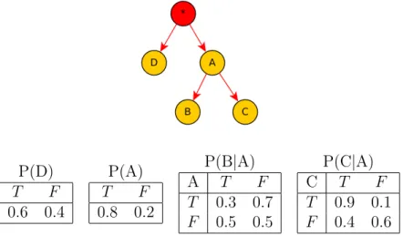
The BN shown in Figure 2.1 is called Earthquake (Korb and Nicholson, 2003), and here we use it as a simple example of the BNs structure and functioning. This network models the behaviour of an alarm that can be activated by burglars, but also has a small probability of being activated by an earthquake, and the reactions of
A B E J M T F 0.001 0.999 T F 0.002 0.998 P(A|B,E) B E T F T T 0.95 0.05 T F 0.94 0.06 F T 0.29 0.71 F F 0.001 0.999 P(J|A) A T F T 0.9 0.1 F 0.05 0.95 P(M|A) A T F T 0.7 0.3 F 0.01 0.99 Figure 2.1: Bayesian networkEarthquake
John and Mary (if they call or not) to the activation of the alarm. All the variables in the BN are Boolean, and they represent the next events:
• B: There is a burglary.
• E: There is an earthquake.
• A: The alarm activates.
• J: John calls.
• M: Mary calls.
As the network domain is discrete, the parameters are represented in CPTs (Figure
2.1). For example, it is easy to see that the probability of activation of the alarm is higher if there is a burglary and there is not an earthquake (P(A = T|B =
T, E = F) = 0.94) than if there is an earthquake and there is not a burglary (P(A =T|B =F, E =T) = 0.29), or that there is more probability that John calls (P(J = T|A = T) = 0.9) than that Mary calls (P(M = T|A = T) = 0.7) if the alarm is activated. The concept of conditional independence is essential to obtain information from BNs. It is defined below:
Definition 1. (Conditional independence): Given a probability distribution P, two random variablesXaandXb are conditionally independent given another random
variable Xc if and only if:
We use(Xa⊥Xb|Xc)P to denote that inP, Xa andXb are conditionally
indepen-dent given Xc.
It is intuitive to see some of the dependences between the variables of the network. For example, it is simple to see that A depends on B, or that J depends on A, but there are some properties of BNs that allow assuming conditional independences among the variables of the network, which is extremely useful in practice. An interesting property of the BNs is the Markov blanket (Pearl,1988).
Definition 2. (Markov blanket): Let B be a BN over X = {X1, X2, . . . , Xn}.
The Markov blanket M B(Xi) of any node Xi ∈ X in B is the set of nodes composed
by the parents of Xi, its children, and the parents of its children. Furthermore, any
node is conditionally independent of the rest when conditioned on M B(Xi).
Although previous works have described sets of axioms that help finding the in-dependences encoded in a BN, as the ones described in Pearl (1995), it is much simpler to use the independence statements from the topological properties of di-rected graphs, and in particular the concept of d-separation (Pearl, 1988; Geiger et al., 1990; Pearl, 1995).
Definition 3. (d-separation): Let XA, XB and XC be three disjoint sets of nodes
in a DAG G. Let T be the set of possibles trials from any nodeXa∈ XA to any node Xb ∈ XB, where a trial in the network is a succession of arcs in G, no matter their
directions. Then XC blocks a trial TI ∈ T if one of the following holds:
1. TI contains a chain Ti−1 →Ti →Ti+1 such that Ti ∈ XC.
2. TI contains a fork Ti−1 ←Ti →Ti+1 such that Ti ∈ XC.
3. TI contains a colliderTi−1 →Ti ←Ti+1 such thatTi and any of its descendants
do not belong to XC.
If all the trials in T are blocked by XC, then XC d-separates XA and XB, which is
expressed by (XA⊥ XB|XC)G.
It is convenient to know the relation between the topological properties of di-rected graphs and the independences of its underlying probability distribution. This relation is defined by the concept of I-map (Pearl, 1988).
Definition 4. (I-map): Let XA, XB and XC be three disjoint sets of nodes in a
(XA⊥ XB|XC)G =⇒ (XA ⊥ XB|XC)P
This means that if G is an I-Map of P, if two set of nodes XA and XB are
d-separated by another set of nodes XC in G, then XA and XB are conditionally
independent in P. This concept allows a formal definition of BNs.
Definition 5. (Bayesian network): LetP be a probability distribution over a set of variables X, then a Bayesian network B is composed of a DAG G and a set of conditional probability distributions such that:
• Every nodeXiinG represents a variable inX, and has a conditional probability
distribution P(Xi|P a(Xi)) associated to it.
• G is a minimal I-map of P. That is no arcs can be removed from G without negating the I-map property.
2.2
Inference in Bayesian networks
The BN model is a complete representation of probability distributions that includes all the variables and their relationships in the model. This allows the calculation of the probability of conditional queries involving any variable of the network.
One of the main objectives of probabilistic models is to answer varied probability queries successfully. For this task it is necessary to perform some kind of reasoning. BNs can deal with diverse problems, and they support deductive, inductive and abductive reasoning. Deductive inference consists of obtaining conclusions from some given events. Inductive reasoning starts from some known events and looks for the causes of these events. Abductive inference tries to find the most likely hypothesis for the given observations.
The most common reasoning problems in BNs are the next:
• Prediction and diagnosis: The inference process for deductive and inductive reasoning in BNs is usually called probability propagation or belief updating. It consists of obtaining the posterior probability P(Q|e) of a set of query variables Qconditioned to a set of evidences e.
• Maximum a posteriori (MAP): It is an abduction problem, usually called par-tial abduction. It consists of searching the most probable configuration of a set of variables in a BN given an evidence.
• Most probable explanation (MPE): It is an abduction problem, usually called total abduction. It consists of searching the most probable configuration of all variables not instantiated in a BN given an evidence. It is a particular case of the MAP problem.
The most desirable methods for probability propagation are those that allow ob-taining the exact value of the probability P(Q=q|E =e) given the structure and parameters of a BN. This type of inference is called exact inference. There are many cases where exact inference is intractable or where an small error in the answers can be handled. Here, approximate inference is usually applied to reduce the computa-tional cost of inference. It consists of obtaining approximate answers that include an error regarding to the BN. The most widely used approximate methods are the stochastic methods, that sample from the network to get an estimation of the result. In this section we describe some of the most popular methods for both exact and approximate inference.
2.2.1
Exact inference
Performing inference directly from BNs using a brute force approach is extremely ex-pensive computationally, so it is rarely used in practice. There are different methods that try to exploit the factorization encoded in the network.
One of the most popular methods is the message passing (MP) algorithm (Pearl,
1986). The MP algorithm is very efficient for the propagation of probabilities in polytrees. The main problem of this method is that it only works for polytrees, and these models are usually not enough for the representation of the knowledge in many real-world domains.
The most widely used approach for performing inference in BNs that are not polytrees is clustering. The main idea of these methods is to compile the network using a clustering technique to group the nodes in a way that the resultant structure is a polytree, and then perform the MP algorithm to the new model. The secondary structures obtained after the compilation of the BNs is another factorization of the joint probability distribution encoded by the BNs, and they are usually called
The JT algorithm was introduced byLauritzen and Spiegelhalter(1988), but there are many different approaches based on this method. The structure of these algo-rithms is similar, and in most cases they follow the next steps:
1. Obtain the moral graph from the BN.
First, the nodes with common parents in the BN are joined with a moral link, so the dependences that would be lost with the transformation of the DAG into an undirected graph are kept.
2. Triangulate the moral graph.
This is a crucial phase, and there are multiple ways of proceeding in this step. In the triangulation achord is introduced in all the cycles with a length bigger than three. These edges are calledfill-ins.
3. Identify the cliques in the triangulated graph.
The nodes of the secondary structure, that are formed for a group of nodes of the BN, are calledcliques. In this step themaximal complete subgraphs should be identified in the triangulated graph. The identification of the cliques is dependent on the triangulation process.
4. Create the junction tree.
The actions necessary for the creation of a valid JT from a set of cliques are the identification of the separators of the JT and the connection of the cliques. 5. Compute the new parameters.
Lastly, the new CPDs should be computed according to the JT structure using the parameters of the BN.
A different approach for the compilation of BNs was proposed inDarwiche(2003). It is based on the representation of the network polynomials that are implicit in the BNs as arithmetic circuits, a useful framework for the graphical representation of polynomials. This work is reviewed in more detail in Chapter 3.
2.2.2
Approximate inference
The purpose of approximate inference is to reduce the computational complexity of the inference process in BNs, that is usually intractable for relatively large networks. The main disadvantage of these methods is that they add an error to the results.
The answers returned by approximate methods are an estimation of the real values. The most popular approximate methods are stochastic. In the stochastic methods the returned values are basically estimated by first, generating samples from the BN, and second, computing the probability of the query from the generated samples. The stochastic methods are based in the Law of large numbers, that states that the estimation should converge to the probability as the number of generated samples grows.
If we imagine that a conditional query P(Q = q|E = e) has been asked to the network, then the most obvious way of getting an approximate response with a stochastic approach is to generate samples from the BN, and then obtain the answer by Nqe÷Ne, where Nqe is the number of samples where Q = q and E = e, and Ne is the number of samples where E = e. This is the general functioning of
stochastic inference methods. Probabilistic logic sampling (PLS) (Henrion, 1988) is an approximate inference method that proceeds in this way, but using an ancestral ordering of the variables to sample from the BN. The PLS algorithm is described in Algorithm2.1.
The main problem of theP LSalgorithm is that all the samples that do not match with evidence e are rejected, which in practice could suppose that, in order to get a satisfactory convergence, a huge amount of samples should be generated. This makes the P LS algorithm intractable or unnecessarily slow in many cases. The
likelihood weighting (LW) algorithm (Fung and Chang, 1989; Shachter and Peot,
1989) overcomes this difficulty by generating weighted samples that always match with evidence e. Each sample and its weight is obtained using the LW particle generation procedure, and then the value of P(q|e) is calculated using the weight of the samples. Algorithm 2.2 describes the likelihood weighting algorithm for m
samples.
Markov chain Monte Carlo (MCMC) methods are one of the most popular ap-proaches for sampling from probability distributions. An stochastic process has the Markov property if in each iteration the future states depend only on the current state, so they are conditionally independent from the past states given the present
Algorithm 2.1 P LS(B,q,e, m)
Input: BN B over X, query variables Q=q, evidenceE =e, number of samples m
Output: Approximate probabilityP(q|e)
1: letX1, . . . , Xn be a topological ordering of X
2: letsmpl be an empty list 3: for i= 1, . . . , mdo
4: for Xj in{X1, . . . , Xn} do
5: letπXj be the configuration ofP a(Xj) in iterationi
6: Generate xij ∼Xj|πXj
7: end for
8: append (xi1, xi2, . . . , xin)to smpl
9: end for
10: letNe be the number of samples in smpl whereE =e
11: letNqe be the number of samples in smpl where E=eand Q=q
12: P(q|e) =Nqe÷Ne
13: return P(q|e)
Algorithm 2.2 LW(B,q,e, m)
Input: BN B over X, query variables Q=q, evidenceE =e, number of samples m
Output: Approximate Probability P(q|e)
1: letX1, . . . , Xn be a topological ordering of X
2: letsmpl be an empty list 3: letwl be an empty list 4: for i:= 1, . . . , m do
5: w:= 1
6: for Xj in{X1, . . . , Xn} do
7: letπXj be the configuration ofP a(Xj) in iterationi
8: if Xj ∈E then
9: letxij be the value ofXj in e
10: w:=w·P(xij|πXj) 11: else 12: Generate xij ∼Xj|πXj 13: end if 14: end for 15: append (xi1, xi2, . . . , xin)to smpl 16: append w towl 17: end for 18: P(q|e) := Pm i=1wl[i]·I(smpl[i]hQi=q) Pm i=1wl[i]
. I = 1 if smpl[i]hQi=q and I = 0 otherwise 19: return P(q|e)
state. The mechanism of MCMC methods consist of a Markov chain that is built in a way that it spends more time in the most important regions of the distribution, so they can sample successfully from complex probability distributions.
Gibbs sampling is a MCMC method that is specially useful for sampling the pos-terior distribution in BNs (Hrycej, 1990). It is a special case of the Metropolis Hastings algorithm (Metropolis et al.,1953;Hastings, 1970) that is simple to apply when the conditional distribution of each variable is easy to sample, which is the case of BNs. The method is divided in a warm-up period, used to converge to the target distribution, and a sampling period, where the useful samples are generated. Algorithm 2.3 applies the Gibbs sampling method to answer any conditional query
P(q|e)in a BNBusingmw as the number of warm-up samples andmas the number
of useful samples.
Algorithm 2.3 Gibbs Sampling(B,q,e, m, mw)
Input: BN B over X ={X1, . . . , Xn}, query variables Q=q, evidence E=e,
Number of samples m, Warm-up samples mw
Output: Approximate Probability P(q|e)
1: letsmpl be an empty list 2: lets0 be a random sample of B
3: for i:= 1, . . . , m+mw do
4: for Xj in{X1, . . . , Xn} do
5: if Xj is in E then
6: letxij be the value ofXj in e
7: else
8: letπXj be the configuration of P a(Xj)in iteration i−1if i6= 1,
or in s0 otherwise 9: Generate xij ∼Xj|πXj 10: end if 11: end for 12: if i > mw then 13: append (xi1, xi2, . . . , xin) tosmpl 14: end if 15: end for
16: letN be the number of samples in smpl
17: letNq be the number of samples in smpl where Q=q
18: return Nq
N
The main problem of approximate methods is that it is complex to estimate the convergence of the samples to the target probability distributions, so many times the number of samples is predefined. If the number of samples is too large the algorithm
can be extremely expensive, and if it is too small the method will not converge to the target probability distribution.
2.3
Scoring metrics
The scoring function has always a mayor impact in the process of learning the structure of BNs with score + search methods. Many different metrics have been proposed over the years, but most of them can be classified as Bayesian metrics or information-theory metrics. Basically, the methods belonging to the first type try find the network that maximizes the posterior probability distribution conditioned to the available data, and those belonging to the information theory metrics base the search on the data compression that can be achieved over the different candidate networks. Carvalho (2009) compares the performance of some methods belonging to both groups of metrics. The results do not show big differences, but in general the results are slightly better for Bayesian scoring functions in large datasets and for information-theory functions in smaller datasets.
While searching for the structure of a BN, the scoring function must evaluate mul-tiple candidate networks, and when facing large datasets or networks the evaluation process is computationally expensive. Therefore, an essential property of the scoring functions is their decomposability. A scoring function is decomposable if the score can be expressed as the sum of a set of scores that depend only on a variable and its parents. If the metric is decomposable, a local change in the network supposes that the metric must compute the evaluation function only for the nodes involved in the change. This supposes a huge improvement in the efficiency of the evaluation process.
Next, we will consider some of the most widely used metrics belonging to both Bayesian and information-theory metrics. All the scoring functions displayed below are decomposable. These metrics are essential for the global purpose of this work, and in Chapter 4 we introduce a metric adapted to our method that is based on some of the scoring functions reviewed in this section. The notation used to define the metrics in this chapter is introduced next:
D: Dataset.
X: Set of variables X ={X1, X2, . . . , Xn}.
xik: Valuek of variable Xi.
wij: Configuration j of the parents of Xi.
θijk: Parameter for the k-th state of Xi conditioned to wij, i.e., P(Xi = xik|P a(Xi) = wij).
ri: Number of states of variable Xi.
qi: Number of possible configurations of the parents of Xi.
Nijk: Number of samples of D where P a(Xi) are in their j-th configuration
and Xi is in itsk-th state. Nij: Pri
k=1Nijk.
N: Number of samples of D.
Nijk0 : Exponents of the Dirichlet prior of θijk. Nij0 : Pri
k=1N
0
ijk.
N0: Equivalent sample size.
2.3.1
Bayesian metrics
The Bayesian scoring functions evaluate each DAG structure by computing the pos-terior probability distribution P(B|D) given a prior distribution over the possible networks conditioned on the data. The next ones are some of the main Bayesian score functions.
The Bayesian Dirichlet (BD) scoring function (Heckerman et al., 1995) faces the optimization problem by making five assumptions related to the user’s prior knowl-edge and the database.
1. The first assumption is calledmultinomial sample. It means that the data can be partitioned into multinomial samples given the structure of B. In other words, it considers that the data is exchangeable, so if an instance of the data is substituted by another instance, the new sample has the same probability as the old one.
2. The second assumption is about parameter independence. It means that the parameters related to each variableXiare independent (global parameter
inde-pendence), and also the parameters related to each configuration of the parents of Xi are independent (local parameter independence).
3. Third, it assumes parameter modularity. It means that the density of the parameters depends only on a variable and its parents.
4. Forth, it assumes that the parameters have a Dirichlet distribution. The Dirichlet distributions are desirable as priors because they are closed under multinomial sampling. This kind of distributions conjugate the prior distribu-tion of the categorical and the multinomial distribudistribu-tions, so if a prior distri-bution is Dirichlet, the posterior, given a multinomial or categorical sample is also Dirichlet.
5. The last assumption is that there iscomplete data. Although this assumption requires a complete database, in Heckerman et al. (1995) it is suggested that incomplete data would not suppose a big obstacle for using the BD function, given that there are many methods that can handle missing data in practice that could be applied in combination with the BD metric. Some examples used to handle missing data are the use of the EM algorithm (Dempster et al.,
1977), or Gibbs sampling (Yi and Li, 2011). Thus, the BD function is:
P(B, D) = P(B)× n Y i=1 qi Y j=1 Γ(Nij0 ) Γ(Nij +Nij0 ) × ri Y k=1 Γ(Nijk+Nijk0 ) Γ(N0 ijk) ! (2.1)
Where Nijk0 are the hyperparameters for the Dirichlet priors of the parameters given the network structure, and Γ is the gamma function.
The BD metric requires the specification of all Nijk, which is intractable in many
cases, making the BD metric useless in practice many times. Nevertheless, there are several scoring functions that are a particular case of the BD metric that have proven to be effective, overcoming this difficulty. The BDe is an specific case of the BD scoring function. With the purpose of making the BD function more useful in practice, the BDe metric includes two extra assumptions.
6. The first one is thelikelihood equivalence; i.e., two DAGs are equivalent if they encode the same joint probability distribution.
7. The second one is the structure possibility. It assumes that for any DAG G, its probability is greater than 0 (P(G)>0).
These assumptions, in combination with the other five assumptions made in the BD metrics, make the BDe metric more tractable in practice than its predecessor, but it keeps requiring some knowledge that is not simple to find. The function that represents the BDe function is the same than the used for BD, but with the assignment Nijk0 = N0 ·P(Xi = xik, P a(Xi) = wij|G), where N0 is a parameter
representing the equivalent sample size for the domain. The equivalent sample size is the sum of all the hyperparameters of the Dirichlet prior distribution conditioned to the network structure.
Another popular Bayesian metric is the K2 (Cooper and Herskovits, 1991, 1992), that is simpler than the previous two. The K2 is also a specific case of the BD function. In particular, it is the result of assigning Nijk0 = 1 in the BD metric. Equation (2.2) represents the K2 scoring function.
P(B, D) = P(B)× n Y i=1 qi Y j=1 (ri−1)! (Nij +ri−1)! × ri Y k=1 (Nijk)! ! (2.2)
2.3.2
Information-theory metrics
This kind of metrics are based in the use of a measure of the data compression of the dataset D obtained with a DAG G, that represents the structure of the learned BN. The main idea of this kind of methods is to find the optimal BNB that encodes the data D.
One way of obtaining the optimal compression of D given B is maximizing the
log-likelihood (LL) of B conditioned to D. The LL scoring function is defined as follows: LL(B|D) = n X i=1 qi X j=1 ri X k=1 Nijklog Nijk Nij (2.3)
As it is shown in Carvalho (2009), adding an arc to B never decreases the LL value, so the use of this function alone usually causes overfitting in the learned model. There are a fair number of scoring metrics based on the LL function that
include a penalty term for the complexity of the network. Equation (2.4) represents this kind of metrics.
LP(B|D) = n X i=1 qi X j=1 ri X k=1 Nijklog Nijk Nij −P enalty(B, D) (2.4)
Some of the most popular scoring metrics that use this strategy are the minimum description length (MDL) (Bouckaert, 1993;Lam and Bacchus,1994), the Bayesian information criterion (BIC) and the Akaike information criterion (AIC) (Akaike,
1974). These functions use|B|, that is, the number of parameters ofB, as a measure of the complexity of the network. |B| is defined by:
|B| =
n
X
i=1
(ri−1)qi (2.5)
On the one hand, when scoring BNs with the BIC function, that is based on the Schwarz Information Criterion (Schwarz, 1978), coincides with the M DL score (De Campos, 2006). The penalty term for both M DL and BIC functions is given by:
P enalty(B, D) = 1
2log (N)|B| (2.6)
On the other hand, the AIC score is slightly different, and its penalty term is represented by:
P enalty(B, D) = |B| (2.7)
An interesting feature of theinformation-theory metrics is that the network likeli-hood and the complexity penalty are obtained independently, and the value of both of them are computed explicitly. As we will see in the further chapters, this prop-erty makes it easier to combine the original scoring function with a new complexity measure of the network.
2.4
Learning the structure of Bayesian networks
In the past years there has been a huge interest in the creation of new methods for learning the structure of BNs from data. Although many different algorithms have been proposed, there are three main approaches that include most of them. The first one is to consider the learning process as a constrain satisfaction problem, trying to get the conditional independences between the variables by using a statistical hypothesis test, and then selecting the model that fits better the dependences and independences obtained in the tests. Two methods that belong to this family are theparents and children (PC) (Spirtes et al., 2000) and the light mutual min (LMM)
(Mahdi and Mezey,2013) algorithms. These techniques do not use an explicit score metric to test the likelihood between the network and the data, and instead they use statistical tests to get the skeleton of the network and then they orientate the edges by recovering the v-structures (Xu →Xv ←Xw) of the network.
The second approach treats the learning process as an optimization problem. These methods, that are called score+search methods, search the BN structure that maximizes a scoring function given the available data. The most popular techniques used for learning the structure of BNs in the space of DAGs are greedy. These methods use heuristic information of the subsequent states in each step of their procedure, and they can be computationally expensive for big sets of variables. An example is the K2 algorithm (Cooper and Herskovits,1991,1992), that goes through each node in a predefined order, adding the best parent until no more improvements can be made or a threshold is reached. Other popular greedy methods are those using hill-climbing (HC) to solve the optimization problem. HC methods explore the search space in a finite number of steps starting from an initial solution. In each step the algorithm considers local changes, selecting the best solution, and it stops when none of the new solutions improves the current one.
The HC method, and unconstrained learning methods for learning BNs in general, are super-exponential in the number of variables of the learned model. This supposes that for big or high-dimensional datasets the learning process is intractable. There are some approaches that include constraints in the search process. This is the case of the constrained hill-climbing (CHC) algorithm (Gámez and Puerta, 2005), that is described in Algorithm2.4. It restricts progressively the number of neighbours to be explored and evaluated, and uses a set of forbidden parents associated to each node that are initialized to empty at the beginning and updated during the search process depending on the metric difference for each local change tested. The main
problem of the CHC method is that the use of the forbidden parents list can cause an early convergence to a local optimum, and it does not assure the return of a minimal I-map. The algorithm receives as an input an initial BN provided by the user, which structure can be a graph without arcs if we are going to learn the network from scratch, and it assumes that the scoring function must be maximized.
Algorithm 2.4 CHC(B, D)
Input: BN B over X ={X1, X2, . . . , Xn}, DataD
Output: BNB0
1: letSold be a list over i= 1,2, . . . , nsuch that Sold[i] =score(Xi, P a(Xi), D)
2: letB0
be a copy ofB
3: letF P be a list of n empty lists . Forbidden parents list
4: OKT oP roceed:=T rue
5: while OKT oP roceed=T rue do
6: . The method bestP redCHC is defined in Algorithm 2.5
7: let Bnew and Snew be the returned values ofbestP redCHC(B, D, Sold, F P)
8: if Pn i=1Snew[i]> Pn i=1Sold[i] then 9: B0 ← Bnew 10: Sold ←Snew 11: else
12: OKT oP roceed:=F alse
13: end if
14: end while
15: return B0
TheiCHC and2iCHC algorithms (Gámez et al.,2011) use an iterative procedure where CHC is applied multiple times, allowing a more probable convergence to a global optimum and assuring the return of a minimal I-map. Algorithm2.6describes the 2iCHC method.
An alternative to the greedy score+search methods are the stochastic search meth-ods. They usually reduce the computational cost of the learning process, but the results that they provide are not always consistent. Simulated annealing is widely used because it adds some intelligence to the stochastic search, trying to reach satis-factory global solutions that are close the global optimum. Wang et al. (2004) used the parallel two-level simulated annealing (Xue, 1993) method for learning BNs. This algorithm uses two levels for each candidate, a lower level and an upper level. The changes on the solutions at each step are made on the upper level. The lower level purpose is to improve the local optimization, so the acceptance of the new solutions depends on the value of the lower level objective function.
Algorithm 2.5 bestP redCHC(B, D, Sold, F P)
Input: BN B, Data D, scoreSold, Forbidden parents F P
Output: Best BN Bnew, Best scoreSbest
1: letchanges be the list of local changes that could be made to B
2: letl be the length of the list of scores Sold
3: letBbest be a copy of B
4: letSbest be a copy of Sold
5: for change inchanges do
6: let Bnew be a copy of B
7: let Snew be a copy of Sold
8: if changeis the addition Xa→Xb then
9: add Xa toP a(Bnew, Xb)
10: Snew(Xb)←score(Xb, P a(Xb), D)
11: if Snew(Xb)< Sold(Xb) then
12: add Xb toF P(Xa)
13: add Xa toF P(Xb)
14: end if
15: else if changeis the deletion of Xa→Xb then
16: deleteXa from P a(Bnew, Xb)
17: Snew(Xb)←score(Xb, P a(Xb), D)
18: if Snew(Xb)> Sold(Xb) then
19: add Xb toF P(Xa)
20: add Xa toF P(Xb)
21: end if
22: else if changeis the reversal of Xa→Xb then
23: deleteXa from P a(Bnew, Xb)
24: add Xb to P a(Bnew, Xb)
25: Snew(Xb)←score(Xb, P a(Xb), D)
26: Snew(Xa)←score(Xa, P a(Xa), D)
27: if Snew(Xb)< Sold(Xb) or Snew(Xa)> Sold(Xa) then
28: add Xb toF P(Xa) 29: add Xa toF P(Xb) 30: end if 31: end if 32: if Pn i=0Snew[i]> Pn i=0Sbest[i] then 33: Bbest ← Bnew 34: Sbest ←Snew 35: end if 36: end for
Algorithm 2.6 2iCHC(B, D)
Input: BN B over X ={X1, X2, . . . , Xn}, DataD
Output: BNB0
1: B0 ←CHC(B, D)
2: B0 ←CHC(B0, D)
3: return B0
The third approach combines the conditional independence tests and the score+search process to obtain the structure of the BN. These methods are called hybrid methods. The max-min hill-climbing (MMHC) (Tsamardinos et al., 2006) is a very popular hybrid method that uses HC for the local search. It first uses statistical hypothesis tests to find the dependencies between the variables and builds the skeleton of the network (edges without orientation) using the max-min parents and children algo-rithm (MMPC). Then, it orientates the arcs of the network using the HC algoalgo-rithm. All these methods, in combination with the scoring functions mentioned before, focus on improving the accuracy of the learned network, producing sometimes over-fitting. As it was said before, some metrics like MDL and AIC include a penalization for the representation complexity of the network using the number of parameters of the model. The representation complexity and the inference complexity are some-times very different for the same model (Beygelzimer and Rish, 2004). This can produce that a model with a reduced number of parameters can be exponentially slower than another with a similar representation complexity and a similar fit. So in practice, performing exact inference in the models learned using this type of meth-ods is usually computationally expensive, and sometimes intractable when the size of the BN is too large. The most common solution is to use approximate inference in these situations, reducing the inference accuracy of the model.
2.5
Learning thin Bayesian networks
When learning BNs from data, many unnecessary dependences are usually stored in the model, increasing the complexity of the network and therefore slowing down the exact inference process. The main motivation of the learning process of BNs is to obtain fitted representations of the data that, when performing inference, obtain results that are accurate with the probability distribution implicit in the data. As we saw before, an accurate model can have a huge inference complexity that can make exact inference intractable, specially if it contains many unnecessary arcs. Exact
inference is always desirable because, although approximate methods are widely used to deal with these type of situations, they include an error that can produce a relevant deterioration of the answers provided by the learned model.
A possible solution to learn models that allow exact inference is to use an esti-mation of the inference complexity in the learning process, with the objective of obtaining fitted models with a tractable inference complexity. Usually, the answers given by an approximate model that uses exact inference are better than the an-swers given by an slightly better fitted model that performs approximate inference. For example, Lowd and Domingos (2010) compared the use of exact inference in approximate models with the use of approximate inference in the original model. The difficulty for this approach is that obtaining a good measure of the inference complexity of a model is not straightforward.
For some of the most popular exact inference methods, such as JTs and some closely related variable elimination techniques, the inference complexity is exponen-tial in the size of the largest clique of the tree. This property is called treewidth, and it is a good indicator of the inference complexity for probabilistic models. In the last years there have been proposed some methods that learn JTs from data using the treewidth of the models to reduce the inference complexity and to make exact inference tractable. The low-treewidth junction trees are usually called thin junction trees (Bach and Jordan,2001). There are some approaches (Chechetka and Guestrin,2008;Elidan and Gould, 2009) that learn JTs using a bounded treewidth.
Vats and Nowak (2014) divided the learning process in multiple subproblems over the separators of the JTs. In order to learn thin junction trees, Shahaf and Guestrin
(2009) used the graph cuts algorithm to select the best separator in each iteration.
Flores (2005) studied the incremental compilation of JTs, and the changes that the addition, reversal or deletion of an arc in a BN could produce on a JT.
A different approach that is not related to JTs was presented byLowd and Domin-gos (2008). It uses the incremental compilation of arithmetic circuits to obtain a tractable model. The ACs are closely related to the work presented in this master thesis, so a detailed review of this model is included in Chapter 3.
Network Polynomials
3.1
Introduction to network polynomials
The probability distribution implicit in any BN can be also represented as a multi-linear function over two types of variables, indicators and parameters:
• Indicators: The evidence indicators I(Xi = xi) are Boolean functions that
receive an instance xi of a variable Xi. They return 1 if xi is in the set of
evidences or if the value of Xi is unknown, and 0 otherwise.
• Parameters: The network parameters P(Xi = xi|P a(Xi) = πi) for each
variable instance xi and each configuration of its parents πi.
This multi-linear function is known as the network polynomial (Darwiche, 2003), and it is defined by the next expression:
P(X1 =x1, . . . , Xn =xn) = n X i=1 Y xi,πi∈ΩXi I(Xi =xi)P(Xi =xi|P a(Xi) = πi) (3.1)
Where we use xi, πi ∈ ΩXi to represent each configuration of a variable and its
parents xi, πi for the variable Xi.
This function represents the joint probability over a set of variables
X ={X1, . . . , Xn}, so the probability of any instance of the variables of the network
can be computed with this formula by setting the indicators to the required values. 27
The instances of the variables are set by assigning the values 1or0to the indicator variables.
Network polynomials allow answering any arbitrary marginal or conditional prob-abilistic query in linear time in the size of the polynomial, but the size of the poly-nomial is exponential in the number of variables of the network.
A
B
P(A) T F 0.6 0.4 P(B|A) A T F T 0.7 0.3 F 0.2 0.8 Figure 3.1: Bayesian network BN1.For example, the network polynomial related to the BN shown in Figure 3.1 can be represented as follows:
P(A, B) =I(A=T rue)I(B =T rue)P(A=T rue)P(B =T rue|A=T rue) +I(A=T rue)I(B =F alse)P(A=T rue)P(B =F alse|A=T rue) +I(A=F alse)I(B =T rue)P(A=F alse)P(B =T rue|A=F alse) +I(A=F alse)I(B =F alse)P(A=F alse)P(B =F alse|A=F alse)
(3.2)
If we need to ask the network polynomial for the probability of the evidence e= (A = T rue, B = F alse), the evidence indicators I(A = T rue) and I(B = F alse)
should be set to 1 and the indicators I(A=F alse)and I(B =T rue) should be set to0. The resulting function is:
P(A=T rue, B =F alse) =P(A=T rue)·P(B =F alse|A=T rue) = 0.6×0.3 = 0.18
If we need to ask for a marginal probability such as P(A = F alse), the only indicator set to 0should be I(A=T rue), and all the other indicators should be set to1. For this query, the resulting function is:
P(A=F alse) =P(A=F alse)P(B =T rue|A =F alse) + P(A =F alse)P(B =
F alse|A=F alse) = 0.4×0.2 + 0.4×0.8 = 0.4
Some other important features of the NPs are the properties of their partial deriva-tives. The function of a NP can be derived with respect to the indicators of the network or the parameters. Deriving the polynomial with respect to evidence indi-cators allows to compute all the partial derivatives with respect some evidence e, and therefore all the evidence instantiations that differ from the evidence indicator in only one variable. This can be useful to solve the maximum a posteriori problem by approximation using local search (Park and Darwiche,2001;Park,2002). For ex-ample, let us consider the partial derivative ofP(A, B)with respect to the indicator
I(A=F alse):
∂P(A, B)
∂I(A=F alse) =I(B =T rue)P(A=F alse)P(B =T rue|A=F alse) +I(B =F alse)P(A=F alse)P(B =F alse|A=F alse)
We have seen before that the value of P(A, B) at e= (A=T rue, B =F alse) is
0.18. Evaluating ∂P(A, B)/∂I(A =F alse) ine would return the value of
P(A=F alse, B =F alse), that is:
P(A=F alse, B =F alse) =P(A=F alse)P(B =F alse|A=F alse) = 0.4×0.8 = 0.32.
The value of∂P(A, B)/∂I(A=F alse)ate= (A=T rue, B =F alse)is given by:
∂P(A=T rue, B =F alse)
∂I(A=F alse) = 0×0.4×0.2 + 1×0.4×0.8 = 0.32
The partial derivatives with respect to the parameters of the network compute the deviation of the function produced by small changes in the parameters. This can be applied to sensitivity analysis. For example, with the purpose of setting bounds to state in which situations the changes in the parameters are relevant,
Chan and Darwiche (2001) analysed the partial derivatives of probabilistic queries with respect to the parameters to study the sensitivity of these queries to changes in the parameters.
3.2
Arithmetic circuits
Although network polynomials have many desirable characteristics for representing BNs, their size is a huge practical issue given that they grow exponentially with the number of variables, making inference nearly intractable for common-size net-works. Trying to overcome this difficulty, Darwiche (2003) proposed an alternative representation of the network polynomials, using arithmetic circuits.
ACs are a popular model for computing polynomials. The formula represented by any network polynomial can be captured in an AC, allowing a more compact representation that uses the distributive properties of the polynomials to reduce the size of the model and therefore the inference complexity. Also, it is interesting to mention that any JT can be interpreted as an AC that factorizes a network polynomial (Park and Darwiche, 2004), so ACs subsume JTs.
ACs are DAGs in which the inner nodes are addition and multiplication nodes and the leaves are numeric variables or constants. The evaluation of the circuits is straightforward and linear in the number of nodes of the graph. The circuit can be evaluated by computing the operations represented by each interior node from the values of its children, starting from the leaves.
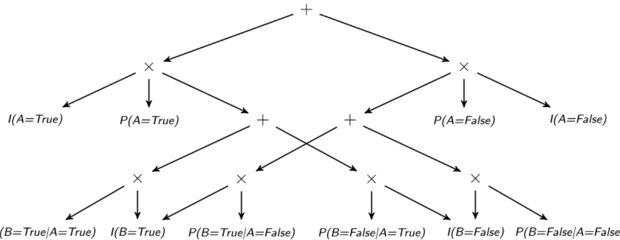
For example, Equation (3.2) can be simplified using the distributive law to refor-mulate the polynomial, as it is shown in Equation (3.3). The new factorization of the polynomial reduces its complexity, leading from the15operations needed to evaluate Equation (3.2) to the 11 operations required to evaluate Equation (3.3). This kind of formulas can be easily represented by arithmetic circuits. The arithmetic circuit that encodes Equation (3.3) is shown in Figure 3.2.
P(A, B) = I(A=T rue)P(A=T rue)×(I(B =T rue)P(B =T rue|A=T rue) +I(B =F alse)P(B =F alse|A=T rue))
+I(A=F alse)P(A=F alse)×(I(B =T rue)P(B =T rue|A=F alse) +I(B =F alse)P(B =F alse|A=F alse))
(3.3)
The reduction of the network polynomial size obtained by their compilation to ACs can be huge for polynomials over medium or big sets of variables, making it possible to represent some network polynomials in linear size in the number of variables,
+ × × + + × × × × P(A=True)
I(A=True) P(A=False) I(A=False)
P(B=True|A=False) I(B=True)
P(B=True|A=True) P(B=False|A=True) I(B=False) P(B=False|A=False)
Figure 3.2: Arithmetic circuit AC1
allowing an inference complexity also linear in the number of variables. As it was stated by Darwiche (2003), ACs can answer any probability query that could be answered by a JT, that are the most popular framework for exact inference in BNs. ACs also provide some useful properties related to the derivatives of the NPs that can help with the resolution of varied problems. As NPs, ACs can be evaluated or derived in linear time with the size of the circuit, making the complexity of inference linear in the size of the circuit and allowing obtaining the partial derivatives of the network polynomial with respect to the variables or the parameters of the network also in linear time. Darwiche (2003) proposed a method that, using a bottom-up evaluation of the circuit and a top-down propagation of the values, obtains all the partial derivatives of an AC given an evidence in linear time with the size of the circuit. In the previous section we showed some of the advantages of using the partial derivatives of NPs.
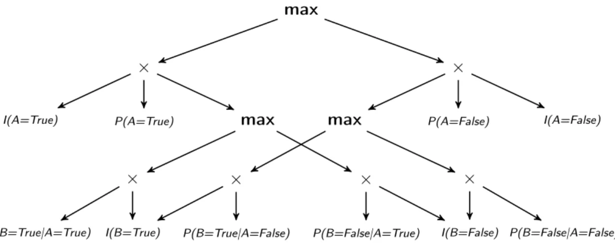
The MPE problem can be solved exactly in linear time using a simple reformulation of an AC. To do this, we would need to use maximizer nodes in the place of the addition nodes of the AC. The resultant model is called maximizer circuit. The maximizer circuit can return all the possible instances of the MPE for any evidence
e required, and also the probability of the MPE for evidence e (Darwiche, 2009). The maximizer circuit that corresponds to the AC used in the previous example is shown in Figure 3.3.
max × × max max × × × × P(A=True)
I(A=True) P(A=False) I(A=False)
P(B=True|A=False) I(B=True)
P(B=True|A=True) P(B=False|A=True) I(B=False) P(B=False|A=False)
Figure 3.3: Maximizer circuit for AC1
3.3
Learning arithmetic circuits
The initial use of ACs in graphical models was for the compilation BNs, separating the offline and the online processes and providing an efficient framework for exact inference. The BNs can be compiled via JTs or by variable elimination to exploit the global structure of the network, butDarwiche(2003) also presented a method to compile the network exploiting its local structure. Learning ACs directly from data is a very challenging task. Darwiche uses the arithmetic circuits as a complementary representation obtained by the compilation of the original model (the BN). The method LearnAC was introduced in Lowd and Domingos (2008). It was the first approach that learns an AC directly from data. LearnAC starts from scratch, with an initial AC that represents the product of the marginal distributionsP(X1, . . . , Xn) =
Q
i
P
xi∈ΩXiI(Xi =xi)·P(Xi =xi), and then starts a greedy search process applying
the best splits in each iteration to add the dependences between variables. The purpose of the LearnAC method is to include the inference complexity of the network in the score metric, and use it to learn tractable models. This score is described in Equation (3.4).
score(C, D) = LL(C|D)−kene(C)−kpnp(C) (3.4) Where:
C: Arithmetic circuit D: Training data sample
LL(C|D): Log-likelihood of the training data
ne(C),np(C): Number of arcs and parameters of the circuit respectively ke,kp: Penalty terms per arc and parameters respectively
The pseudocode of LearnAC is shown in Algorithm 3.1. The key of this algo-rithm is the splitting procedure, that updates the circuit incrementally. An split
S(C, P, Xi) conditions the parameters in P in the variable Xi, which in a Bayesian
network can be interpreted as arc additions. The experimental results presented by Lowd and Domingos (2008) show that the circuits obtained by learnAC have a tractable inference complexity, and exact inference in the obtained AC is more efficient than approximate inference using Gibbs sampling in BNs learned by other popular methods.
Algorithm 3.1 LearnAC(X, D)
Input: set of variables X ={X1, X2, . . . , Xn}, DataD
Output: Arithmetic circuit C
1: letC be an arithmetic circuit representing the product of marginals. 2: OKT oP roceed:=T rue
3: while OKT oP roceed=T rue do
4: let Cbest be a copy of C
5: OKT oP roceed:=F alse
6: for each valid split S(C, P, Xi) do
7: C0 ←SplitAC(C, S(C, P, Xi))
8: if score(C0, D)> score(C
best, D) then
9: Cbest ← C0
10: OKT oP roceed:=T rue
11: end if
12: end for
13: if OKT oP roceed=T rue then
14: C ← Cbest 15: end if
16: end while
There are some other interesting works related to ACs learning. In Lowd and Rooshenas (2013), the LearnAC algorithm was adapted to learn Markov networks instead of BNs as ACs. The work presented by Lowd and Domingos (2010) stud-ied the compilation of BNs with a very high treewidth, where the AC compilation proposed by Darwiche (2003) is intractable. Trying to overcome this difficulty they presented three new methods that apply approximate compilation, allowing exact inference in the approximate model. These algorithms sample from the original net-work to obtain data samples and then they apply the LearnAC algorithm to learn an AC.
3.3.1
Example of split
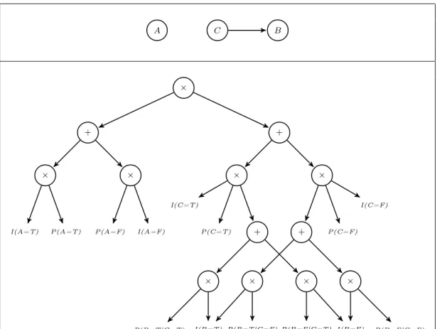
The splitting procedure is the main key of learnAC method. Let us focus on the AC shown in Figure 3.4. It represents the polynomial P(A, B, C) = (P
a∈ΩAI(a)P(a))·
(P
c∈ΩCI(c)P(c)·(
P
b∈ΩBI(b)P(b|c))). The addition of the arc B → A to the BN
corresponds to the splitS(C,{P(A=T rue), P(A=F alse)}, B). So the parameters of A are conditioned to variable B, and now there must be a summation over all the instances of B above the parameters of A in the AC. The splitting procedure of LearnAC obtains an efficient factorization of the network polynomial. The resultant AC is shown in Figure 3.5, and the polynomial represented by the updated AC is
P(A, B, C) =P b∈ΩBI(b)( P a∈ΩAI(a)P(a|b))·( P c∈ΩCI(c)P(c)P(b|c)).
It must be noted that Figure3.5only shows the part of the AC where the indicator of B is I(B = T rue). The other part of the circuit is identical to the part shown, but usingB =F alseinstead ofB =T ruein all the parameters or indicators related to variableB. In Figure 3.4 and Figure3.5 we useT to refer to True andF to refer toFalse.
A C B
×
+ +
× ×
I(A=T) P(A=T) P(A=F) I(A=F)
× ×
P(C=T) + + P(C=F)
I(C=T) I(C=F)
× × × ×
P(B=T|C=T) I(B=T) P(B=T|C=F)P(B=F|C=T) I(B=F) P(B=F|C=F)
Figure 3.4: LearnAC example. BN (top) and AC (bottom) before split.
C B A
×
+ +
× ×
I(A=T) P(A=T|B=T) P(A=F|B=T) I(A=F)
× × P(C=T)P(B=T|C=T) P(B=T|C=F) P(C=F) I(C=T) I(C=F) I(B=T) + × I(B=F) . . .
Polynomial Trees
One of the disadvantages for the representation of BNs as ACs is that they are not a framework dedicated to probability distributions (Jaeger et al.,2006), because they can represent any kind of polynomials, including those that do not encode a network polynomial. For the task of learning a probabilistic model from data, it is essential to operate over a delimited search space, and the search space of arithmetic circuits is not bounded to the space of probability distributions. This fact makes the task of learning ACs directly from data very difficult. As we saw in Chapter 3, state-of-the-art methods for learning ACs from data like LearnAC are greedy methods that proceed by conditioning variables of the network to other variables. This is done by splitting the parameter nodes corresponding to the conditioned variable into the conditioning variable. The operations that LearnAC considers in each step are limited, including only the arc additions that produce a valid split of the current circuit. It would be very challenging to create flexible algorithms for learning ACs capable of doing and evaluating any possible movement during the search, including all the arc additions, deletions or reversals that maintain the integrity of the network. State-of-the-art methods for learning BNs usually consider all these possibilities.
Another disadvantage of the ACs is their lack of expressiveness. They are thought as a complementary model for BNs, but given that they can have a huge number of nodes and edges, it is extremely unintuitive to identify the conditional depen-dences between the variables of the network by only looking at the representation of the circuit, or to combine the graphical information of an AC with the graphical information provided by a BN.
The purpose of this master thesis is to find a new representation of the network polynomials that keeps the main properties of the ACs using a simple representation, easy to understand and highly compatible with the graphical representation of BNs. To achieve these goals, we propose a new graphical model complementary to BNs for representing discrete probability distributions, which we callpolynomial trees (PTs). As ACs, each PT encodes a compact network polynomial and is associated to a BN. A PT consists of the next elements:
1. A set of nodesXP, including a root node∗and a nodeXi ∈ X for each variable
of the probability distribution.
2. An indicator variableI(Xi) associated to each node Xi ∈ X. Each indicator
can take the value of any state of the variable Xi and the value N one if it is
not set.
3. A set of directed arcs that represent the operation dependences and ordering over all the variables of the network, forming a tree structure that connects all the nodes of the network, where the root node∗ is the ancestor.
4. An associated Bayesian network B over X. B is composed of a DAG repre-senting the dependences in the network and of a set of parameters for each nodeXi ∈ X.
Basically, the complete graphical representation of a PT should consist of a DAG representing the dependences in the network and a tree representing the inference operation order. It is important to mention that there are usually multiple valid PTs for each BN, because there are multiple possible orders to perform exact inference on each network, so a difficulty for learning PTs would be to find those trees that require a lower number of operations per inference query.
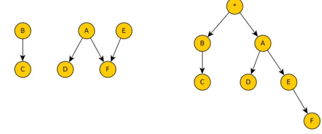
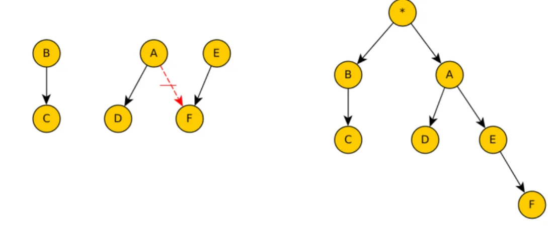
As an example, let us focus on the structure of the BN BN2, that is shown in Figure 4.1. The network has 9 variables, and we will assume that all the variables are Boolean, and therefore they can only take the values True or False.
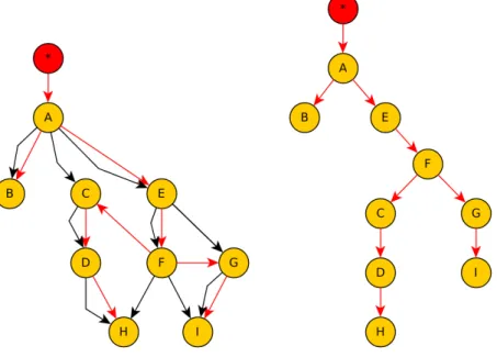
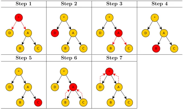
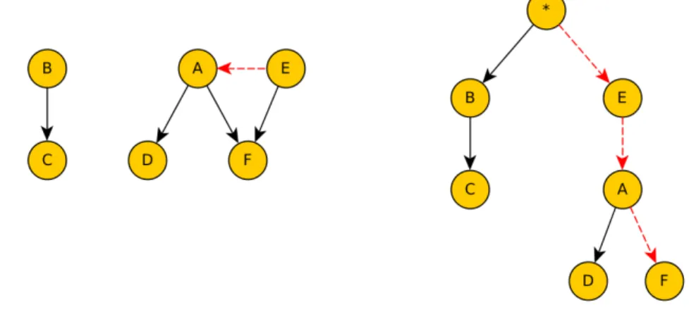
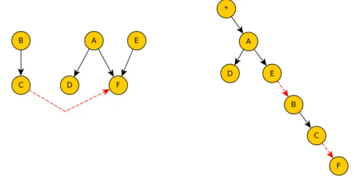
Figure 4.2 shows a PT that represents a valid operating order for BN2. It is possible to distinguish a DAG (in black), that shows the dependences between the variables of the network, and a tree (in red) that shows the operations chain used to perform exact inference in the PT. The root node∗ represents the first operation to be executed in the inference procedure.
Figure 4.1: Structure of the Bayesian network BN2.
Figure 4.2: Combination of BN and PT for BN2 (left), and only the PT (right).
PTs are a complementary model for BNs, and each PT is associated to a BN. The soundness of a PT is the property that assures that any probabilistic query that could be answered by a BN B can be answered with the same response by its associated PT P. As we will see in the next section, the inference process proposed for PTs consists of a top-down process for the propagation of the indicators and a bottom-up process for the computation of the probabilities. In order to compute the parameters of a node Xi, it is necessary that the indicators rel