Network Simplification: the Gaussian Diamond
Network with Multiple Antennas
Caner Nazaroglu
Middle East Technical University Ankara, Turkey
Javad B. Ebrahimi, Ayfer ¨
Ozg¨ur, Christina Fragouli
EPFL, Lausanne Switzerland
{javad.ebrahimi, ayfer.ozgur, christina.fragouli}@epfl.ch
Abstract—We consider theN-relay Gaussian diamond network when the source and the destination have ns ≥2 and nd ≥2 antennas respectively. We show that whenns=nd= 2and when the individual MISO channels from the source to each relay and the SIMO channels from each relay to the destination have the same capacity, there exists a two relay sub-network that achieves approximately all the capacity of the network. To prove this result, we establish a simple relation between the joint entropies of three Gaussian random variables, which is not implied by standard Shannon-type entropy inequalities.1
I. INTRODUCTION
Consider a source communicating to a destination with the help of wireless relays. With network simplification we refer to the problem of removing a number of wireless relays while maintaining a desired fraction of the wireless network capacity. Our ultimate goal is to understand by how much and how we can prune an arbitrary wireless network; here we present results for special classes of Gaussian diamond networks.
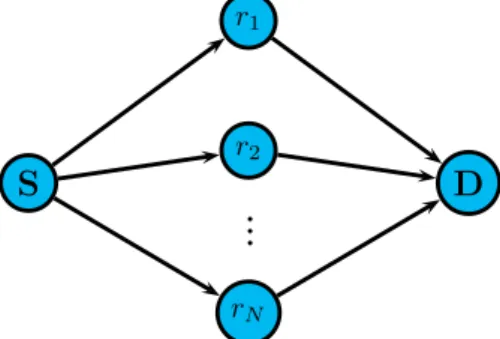
Our first results in this direction, presented in [1], assumed that all nodes have single antennas. The source is connected to the relays through a broadcast channel, while the relays are connected to the destination through a multiple-access channel, as depicted in Fig. 1. In this paper, we take the next natural step, and consider the case where the source has ns transmit antennas while the destination has nd receive antennas.
We start by formulating theN-relay network simplification problem as a combinatorial problem, similar to our approach in [1]. To do so, we provide a simplification result for the point-to-point MIMO channel. We show that if we have nt transmit and nr ≥nt receive antennas, there exists a subset ofntreceive antennas which alone achieve the capacity of the original (nt×nr) MIMO channel within a gap ofntlog((nr−
nt+ 1)nt) +ntlognt bits/s/Hz. An analogous result holds when nt≥nr.
However, to proceed from this point, combinatorial argu-ments similar to [1] (wherens=nd= 1), cannot be directly applied. This is because multiple antennas introduce more degrees of freedom in the network. The channel from the source to each relay (or from each relay to the destination node) is no longer characterized by a single coefficient (the channel gain), but by a vector of coefficients. Therefore, it 1This work was supported by the ERC Starting Grant Project NOWIRE ERC-2009-StG-240317.
S
r1 r2...
rND
Fig. 1. The GaussianN-relay diamond network. The source withnstransmit
antennas is connected toNsingle antenna relays through a broadcast channel;
the relays are connected to the destination which has nd receive antennas
through a multiple-access channel.
is not only the configuration of the channel gains, which corresponds to the magnitudes of these vectors, but also the orientation of the vectors that can lead to “small” capacities for the subnetworks.
Our main result is to show that, whenns=nd= 2and the individual multiple-input-single output (MISO) channels from the source to each relay and the single-input-multiple-output (SIMO) channels from each relay to the destination have the same capacity, there exist two relays that together approxi-mately achieve the whole capacity of the network. That is, to understand the new dimension of channel orientations that comes into play, we focus on the case where the magnitudes of the channel coefficient vectors are assumed to be equal while their orientations are arbitrary. In this case, for ns=nd= 2, it is clearly necessary to use at least two relays to approach capacity, since we have two degrees of freedom in the system. We show that this is also sufficient, which is non-trivial since arbitrary orientations of the channel vectors could potentially lead to small capacities for all 2-relay subnetworks.
The main ingredient of our proof comes from establishing a simple relation between the joint entropies of three Gaussian random variables, which is not implied by standard Shannon-type entropy inequalities, and might be of interest in itself. We show that if X, Y, and Z are three jointly Gaussian random variables with I(X;Y) smaller than both I(X;Z)
andI(Y;Z), thenmin(I(X;Z), I(Y;Z))≤I(X;Y)+2bits. Intuitively, ifX andY give little information about each other,
Z can not simultaneously give a lot of information about both
X andY.
We finally show that, our result does not hold if we remove
the restriction of equal capacities for the individual links. We provide an example configuration for the N-relay diamond network with ns = nd = 2, where all 2-relay subnetworks can at most achieve half the capacity of the whole network. A natural question in this case is whether we can always find 2
relays that would allow us to achieve half the network capacity. We are able to answer this question positively for the case when the diamond network contains3 or 4relay nodes.
The paper is organized as follows. Section II provides our model; Section III summarizes our main result; Section IV presents a simplification result for the MIMO channel; Sec-tion V formulates the combinatorial problem for the N-relay diamond network; Section VI proves our main result and Section VII considers arbitrary diamond networks withN ≤4.
II. MODEL
We consider the Gaussian N-relay diamond network de-picted in Fig. 1 where the source node S wants to communi-cate to the destination nodeDwith the help ofNrelay nodes, denotedN. Assume that the source node is equipped withns transmit antennas and the destination node is equipped with
ndreceive antennas, while each relay has a single transmit and receive antenna. We assume that N ≥max(ns, nd), typically
N % max(ns, nd). Let Xs[t] and Xi[t] denote the signals transmitted by the source node S and the relay node i∈ N respectively at time instant t ∈ N. Similarly, Yd[t] and Yi[t] denote the signals received by the destination nodedand the relay nodeirespectively. The transmitted signalXi[t]by relay
i is a causal function of its received signalYi[t]. We have
Yi[t] =hisXs[t] +Zi[t], Yd[t] = N ! i=1 h†diXi[t] +Z[t],
wherehisdenotes the1×nscomplex channel vector between thenstransmit antennas at the source node and the relay node
i and h†di denotes nd ×1 complex channel vector between the relay node i and the nd receive antennas at destination node. Note that Xs andYd are vectors of length ns and nd respectively, while Xi and Yi are scalars. Zi[t], i ∈ N are independent and identically distributed white Gaussian random processes of power spectral densityN0/2Watts/Hz. Similarly
Z[t] is a length nd circularly symmetric Gaussian vector of identity covariance matrix and power spectral density N0/2 Watts/Hz. All nodes are subject to an average power constraint
P and the narrow-band system is allocated a bandwidth ofW. Note that the equal power constraint assumption is without loss of generality as the channel coefficients are arbitrary. We assume that the channel coefficients are known at all the nodes. We denote the capacity of the multiple-input single-output channel between the source node and the relay ibyαi, i.e.,
αi= log(1 +SNR||his||2), where SNR= P
N0W. Similarly, the capacity of the individual SIMO channel from the relay node ito the destination node is given by
βi= log(1 +SNR||hid||2).
III. MAINRESULT
The following theorem summarizes our main result. Theorem 3.1: Consider the GaussianN-relay diamond net-work with capacityC, wherens= 2,nd = 2andαi=αand
βi =β for all i ∈ N. Then, there exists a 2-relay diamond subnetwork such that its capacityC2 satisfies
C2 ≥ C −G,
whereG= 18 + 4 log(N−1)is a universal constant indepen-dent of the channel configurations and the operating SNR.
When theαi’s and βi’s are not equal, there exist configu-rations of the N-relay diamond network with ns = nd = 2 such that every2-relay sub-network provides at most half the capacity. We provide such an example in Section VII. In the same section, we also prove the following proposition.
Proposition 3.1: In every Gaussian N-relay diamond net-work with capacityC, wherens= 2,nd = 2andN ≤4, there exists a 2-relay diamond subnetwork such that its capacityC2 satisfies
C2 ≥
1
2C −G,
whereG= 11 + 2 log(N−1)is a universal constant indepen-dent of the channel configurations and the operating SNR.
IV. MIMO CHANNELSIMPLIFICATION
Consider a MIMO channel withnttransmit andnrreceive antennas and thenr×nt channel matrix denoted byH. We have Y = HX +Z. The capacity of this channel is well known to be [4]
Cnr×nt = max
Q≥0, tr(Q)≤SNRlog det(I+HQH
†) (1) whereQis a positive semidefinite matrix, tr(Q)is the trace of the matrixQ, SNR= P
N0W andH
† denotes the conjugate transpose ofH.
Theorem 4.1: Consider an nr ×nt MIMO channel with capacityCnr×nt in (1) and assume nr≥nt. LetRbe the set
of receive antennas. Let
Cnt×nt = max
A⊆R |A|=nt
log det(I+SNRHAHA†),
where HA is the sub-MIMO channel from the nt transmit antennas to the nt receive antennas in the set A ⊆ R. We have
Cnt×nt−G0≤Cnr×nt ≤Cnt×nt+G1 (2)
whereG0=ntlogntandG1=ntlog((nr−nt+ 1)nt). The above theorem suggests that the capacity loss incurred by using a subset of the receive antennas in an nr ×nt MIMO channel, with nr ≥ nt, is bounded by a universal constant independent of the channel gains and the operating SNR, if the number of selected receive antennas is larger than or equal tont. This implies that in the high capacity regime using onlymin(nt, nr)antennas on both sides of the channel is approximately optimal. Antenna selection for the MIMO channel has been extensively studied in the literature [7], [8],
[9], [10]. A similar result to Theorem 4.1 appears in [2]. The proof of the theorem is given in [12].
An analogous result to Theorem 4.1 holds for the case of
nt > nr: Let Cn%r×nt be the capacity of a MIMO channel
given in (4.1) but with a total power constraint ntP instead of P.2 Let
Cn%t×nt = max
A⊆T |A|=nr
log det(I+SNRHAHA†), whereT is the set of nttransmit antennas. We have
Cn%t×nt ≤C
%
nr×nt ≤C
%
nt×nt+G2 (3)
whereG2=nrlog((nt−nr+ 1)nr) +nrlognr. V. RELAYNETWORKS WITHMULTIPLEANTENNAS In this section, we use the MIMO channel simplification result of Section IV, to derive lower and upper bounds on the capacity of the diamond relay network. These simple lower and upper bounds allow us to pose the question of interest as a purely combinatorial problem. We provide solutions to this combinatorial problem in certain special cases in Sections VI and VII. The flow of our analysis is analogous to [1]. A. Approximate Capacity of a Diamond Relay Network
Consider a subset Γ ⊆ N of the relay nodes, such that |Γ|= k. For a subset Λ ⊆Γ, define Λ =Γ \Λ. LetCΓ be
the capacity of the k-relay diamond sub-network (assuming the remaining N −k relay nodes are not used for the S-D
communication). Then ˜ CΓ−G4≤CΓ≤C˜Γ+G3, (4) where C˜Γ= min Λ⊆Γ " max A⊆Λ¯ |A|≤ns log det(I+SNRHASHAS† ) + max A⊆Λ |A|≤nd log det(I+SNRHDAHDA† ) # , (5) andG4= 3k+nslogns andG3=nslog((k−ns+ 1)ns) +
ndlog((k−nd+ 1)nd) +ndlognd.HAS is the cooperative MIMO channel between the source and a subsetA⊆Γof the relay nodes, with columns his, i ∈ A. HDA is analogously defined. To prove (4) we combine the information theoretic cutset upper bound on the capacity of the k-relay diamond network with the lower and upper bounds on MIMO capacity in (2) and (3). To obtain the lower bound in (4), we also refer to the result of [6] that the cutset upper bound is achievable within 3k bits/s/Hz.
B. A Combinatorial Problem
In the previous section, we have seen that up to a total gap ofG4+G3, the capacity of ak-relay diamond network behaves approximately like (5). In the rest of the discussion we will concentrate on this approximate form of the capacity. Note that if we establish a result for the approximate capacity, we 2We use this result to simplify the cooperative MIMO channel between the
ntrelay nodes and the destination node in the next section. Since every relay
node has powerP, the cooperative MIMO channel has total powerntP.
can translate it to a constant gap result for the actual capacity: LetC denote the capacity of the network with all relays, i.e.
C=CN, and letCkbe the capacity of thek-relay subnetwork with the largest capacity, i.e.,
Ck = max
Γ⊆N |Γ|=k
CΓ. (6)
Let C˜ = ˜CN and C˜k = maxΓ⊆N |Γ|=k
˜
CΓ be the corresponding
approximate capacities. If we can show that
˜
Ck ≥rkC˜−γk, (7) using the lower and upper bounds bounds in (4) yields
Ck≥rk(C−G3)−γk−G4. (8) Let us introduce the notation
α(A) = log det(I+SNRHASHAS† ),
β(A) = log det(I+SNRHDAHDA† ), (9) where A ⊆ N. α : 2n → R+ and β : 2n → R+ are two positive set functions defined on subsets of N. C˜Γ can be
rewritten in terms of these set functions as
˜ CΓ= min Λ⊆Γ " max A⊆Λ¯ |A|≤ns α(A) + max A⊆Λ |A|≤nd β(A)#.
In the rest of the paper, we will aim to establish a universal lower bound onrk and a universal upper bound onγk in (7), independent of the particular channel configurations and the operating SNR, by using the properties of the set functionsα
andβ. By (8), this translates to a worst case guarantee on the fraction of the capacity we can achieve with k relays within a constant additive gap. Since in the rest of the discussion, we only work in terms of the approximate capacitiesC˜Γ, we
simply refer to it as the capacity of the subnetworkΓ. The set functions in (9) can be associated with the joint entropies of the random variables
Ysi=hsi
√
SNRXs+Zsi, Yid=hdi
√
SNRXd+Zdi, where Xs and Xd are circularly symmetric Gaussian ran-dom vectors of length 2, zero mean and identity covariance matrix. Zsi and Zdi are independent circularly symmetric Gaussian random variables of unit variance. We haveα(A) =
H(Ysi, i ∈ A)− |A|log(2πe) and β(A) = H(Yid, i ∈
A)−|A|log(2πe). Therefore these set functions should satisfy certain properties satisfied by the joint entropies of a set of Gaussian random variables. In particular, they have to satisfy the following submodularity properties, also called the Shannon inequalities for entropy:
(i) α(A1)≤α(A2) if A1⊆A2.
(ii) α(A1∪A2)≤α(A1) +α(A2)−α(A1∩A2). Similar relations hold for the functionβ.
However, the above properties are not sufficient to prove the result in Theorem 3.1; below we establish an additional property we will need. The proof is provided in Appendix A.
Lemma 5.1: LetX, Y, Z be jointly Gaussian random vari-ables. Let I(X, Y) = min(I(X, Y), I(X, Z), I(Y, Z)). Then
min(I(X, Z), I(Y, Z))≤I(X, Y) + 2bits.
When H(X) = H(Y) = H(Z), the lemma reduces to the following: If H(X, Y) = max(H(X, Y), H(X, Z), H(Y, Z)), then
H(X, Y)≤max(H(X, Z), H(Y, Z)) + 2. (10) Intuitively, the lemma suggests that if the mutual information between X and Y is small, i.e. X and Y are close to be independent, then Z can not give a lot of information simultaneously about both of them.
VI. PROOF OFTHEOREM3.1
Let us write αi for α({i}) and αi,j for α({i, j}). When
αi =αfor alli∈N, (10) implies the following relation for any three relays i, j, k∈N: Letαi,j= max(αi,j,αj,k,αi,k), then
αi,j≤max(αj,k,αi,k) + 2. (11) Similar relations hold forβ. Using this property, we will prove that C˜2≥C˜−4 in this case.
Note that when αi = αand βi =β, by the property (ii), any αi,j≤2αandβk,l≤2β. Therefore, for anyΓ⊆N,
˜
CΓ = min(max
i,j∈Γαi,j,k,lmax∈Γβk,l). (12)
That is the min cut is eitherΛ=∅ orΛ=Γ, since the value of any other cut is at least α+β≥2 min(α,β).
Let1,2∈N be the pair of relays with the largest αvalue, i.e.α1,2= maxi,j∈Nαi,jand similarlyβ3,4= maxk,l∈Nβk,l. We assume that the pairs with maximum αandβ values are disjoint since this is the most difficult case to deal with. Note that by (12), α1,2 ≥C˜ and β3,4 ≥C˜. Below we argue that there exists a two relay subnetwork Γ∈{1,2,3,4} such that
˜
CΓ≥C˜−4. We assume thatβ1,2<C˜−4andα3,4<C˜−4, since otherwise we are done.
• By applying (11) toα({1,2,3}), eitherα1,3≥C˜−2 or α2,3≥C˜−2. W.l.o.g, assumeα1,3≥C˜−2. • Thenβ1,3<C˜−4, otherwise C˜{1,3}≥C˜−4. • By applying (11) to β({1,3,4}), we haveβ1,4≥C˜−2. • Thenα1,4<C˜−4, otherwiseC˜{1,4}≥C˜−4. • By applying (11) toα({1,2,4}), we haveα2,4≥C˜−2. • By applying (11) toα({2,3,4}), we haveα2,3≥C˜−4. • Also, β2,4<C˜−4, otherwiseC˜{2,4}≥C˜−4. • By applying (11) to β({2,3,4}), we haveβ2,3≥C˜−2. Combined with α2,3≥C˜−4, this yieldsC˜2≥C˜−4.
VII. ARBITRARYDIAMONDNETWORKS WITH
ns= 2, nd = 2ANDN ≤4
When the equality constraint on the individual capacities
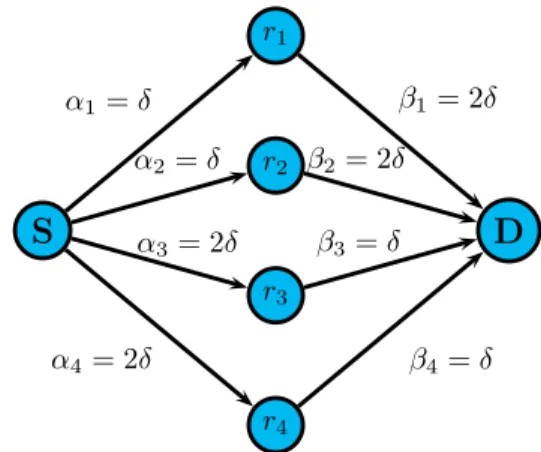
αi=αandβi=β is removed, the assertion in Theorem 3.1 does not hold anymore. Consider the 4-relay network in Fig 2, and assume that, as illustrated also in the figure,α1=α2=δ,
α3 =α4 = 2δ, β1 =β2 = 2δ,β3 =β4 =δ. These are the capacities of the individual channels from the source to each relay, and from each relay to the destination.
S
r1 r2 r3 r4D
α1=δ α2=δ α3= 2δ α4= 2δ β1= 2δ β2= 2δ β3=δ β4=δFig. 2. An instantiation of a diamond network with4relays.
Now assumens =nd = 2, and moreover that α1,2 = 2δ,
α1,3 = 2δ, α1,4 = 3δ, α2,3 = 3δ, α2,4 = 3δ, α3,4 = 4δ. Symmetrically, assume β1,2 = 4δ, β1,3 = 3δ, β1,4 = 2δ,
β2,3 = 2δ, β2,4 = 3δ, α3,4 = 2δ. (One can easily verify that these assignments satisfy the conditions in (i) and (ii) and Lemma 5.1. Indeed, we can also specify the channel vectors that would lead to the set functions given above. Consider for example h1s= [a0],h2s= [0a],h3s= [a2 0],h4s= [0a2] andhd1= [a20],hd2= [0a2],hd3= [0a],hd4= [a0]when
a % 1.) Then the capacity of this network becomes 4δ. By using a single relay we can at most achieveδ, a fraction1/4
of the total capacity. This fact illustrates that the conclusions of [1] do not extend to the case of multiple antennas. On the other hand every two-relay subnetwork has capacity 2δ. Thereforerk = 1/2for this configuration and the conclusion of Theorem 3.1 also does not hold.
When ns = nd = 2, we can show that this example corresponds to a worst case configuration, i.e. rk ≥ 12 when
N ≤4for any configuration of the channels. Below we prove Proposition 3.1 forN = 3. The proof follows similar lines for
N = 4.
Proof of Proposition 3.1:We will rely on a weaker version of the properties (i) and (ii) for the set functions α and β. Namely,
max{αi,αj}≤αi,j ≤αi+αj. (13) Assume we have a 3-relay network with capacity C˜, and its every two-relay subnetwork has capacity< C˜
2. Then: • There exists i ∈ {1,2,3} such that αi ≥ C/˜ 2, w.l.o.g.
assume it is i = 1: Otherwise the cut Λ = ∅, yields a value strictly smaller than C˜ contradicting with the assumption that the capacity of the network isC˜. • β1 <C/˜ 2: Otherwise, C˜1 ≥C/˜ 2, leading to a
contra-diction.
• Since the capacity of the 2-relay subnetwork with relays {2,3} is <C/˜ 2, we either have α2,3 <C/˜ 2 or β2,3 <
˜
C/2 or α2+β3 < C/˜ 2 or β2+β3 < C/˜ 2. All these cases combined with β1 <C/˜ 2 and the condition (13) lead to a cut for the 3-relay network with value < C˜
which contradicts with the fact that the capacity of the network isC˜. This concludes the proof of the proposition.
REFERENCES
[1] C. Nazaroglu, A. ¨Ozg¨ur, C. Fragouli,Wireless Network Simplification: the GaussianN-Relay Diamond Network, IEEE Int. Symposium on
Information Theory (ISIT), St-Petersburg, 2011.
[2] Y. Jiang M. K. Varanasi, The RF-chain Limited MIMO System - Part I: Optimum Diversity-Multiplexing Tradeoff, IEEE Trans. on Wireless Communications, Vol. 8(10), Oct. 2009.
[3] Cover, T.M, Thomas J. A., Elements of Information Theory, Wiley & Sons Inc., 1991.
[4] D. Tse and P. Viswanath, Fundamentals of Wireless Communication, Cambridge University Press, 2005.
[5] S. Avestimehr, S. Diggavi and D. Tse, Wireless network information flow: a deterministic approach, eprint arXiv:0906.5394v2 - arxiv.org. [6] A. ¨Ozg¨ur, S. Diggavi,Approximately Achieving Gaussian Relay Network
Capacity with Lattice Codes, Proc. IEEE Int. Symposium on Information Theory, Austin, June 2010.
[7] A. Gorokhov, D. A. Gore, A. J. Paulraj, “Receive Antanna Selection for MIMO Spatial Multiplexing: Theory and Algorithms” IEEE Trans. on Signal Processing, Vol. 51(11), Nov. 2003.
[8] A. Gorokhov, D. A. Gore, A. J. Paulraj, “Receive Antenna Selection for MIMO Flat-Fading Channels: Theory and Algorithms” IEEE Trans. on Information Theory, Vol. 49(10), Oct. 2003.
[9] A. F. Molisch, M. Z. Win, Y.-S. Choi, J. H. Winters, “Capacity of MIMO Systems with antenna Selection” IEEE Trans. on Wireless Communication, Vol. 4(4), Jul. 2005.
[10] S. Sanayei, A. Nosratinia, “Antenna selection in MIMO systems”, IEEE Communications Magazine, Vol. 42(10), Oct. 2004.
[11] Y. P. Hong, C.-T. Pan, “Rank-Revealing QR Factorization and the singular value Decomposition”, Mathematics of Computation, Vol. 58, No. 197, pp. 213-232, Jan 1992.
[12] C. Nazaroglu, A. ¨Ozg¨ur, J. B. Ebrahimi, C. Fragouli, “Network simpli-fication: the Gaussian diamond network with multiple antennas”, EPFL Technical Report, 2011.
APPENDIXA PROOF OFLEMMA5.1
The joint entropy of the three jointly Gaussian random variables is given by
H(X, Y, Z) = log det((2πe)K)
whereKis the3×3covariance matrix of the three variables. Note that since K is positive semidefinite, it can be written as K = SS†. Let s1, s2, s3 ∈ C3 denote the rows of S. The joint entropy of a subset A of these random variables
X, Y, Z is given byH(A) = log det((2πe)KA)whereKA is the corresponding submatrix ofK.
Let I(X, Y) = min(I(X, Y), I(X, Z), I(Y, Z)) and let
X, Y correspond to the upper left 2×2 submatrix of K. We have
I(X, Y) =h(X) +h(Y)−h(X, Y)
= log(||s1||2) + log(||s2||2)−log(||s1||2||s2||2−|< s1, s2>|2)
=−log(1−cos2(f(s1, s2))), where f(s1, s2) = arccos $ |< s1, s2>| ||s1||||s2|| % .
Note that for I(X, Y) to be minimal we have
f(s1, s2) = max(f(s1, s2), f(s1, s3), f(s2, s3)). Below in Proposition A.3, we prove that for any three vectors
s1, s2, s3 inCn, we have
f(s1, s2)≤f(s1, s3) +f(s2, s3).
Thereforemax(f(s1, s3), f(s2, s3))≥f(s1, s2)/2. We have
min(I(X, Z), I(Y, Z))≤ −log(1−cos2(f(s1, s2)/2))
=−log(sin2(f(s1, s2)/2))≤I(X, Y) + 2,
sincelog(sin2(f(s1, s2)))−log(sin2(f(s1, s2)/2))≤2.This concludes the proof of the lemma. !
For two complex vectors a, b∈Cn, the quantity f(a, b) is roughly like the angle between these vectors. Below we prove that this quantity satisfies the triangle inequality:
Note that 0 ≤ f(a, b) ≤ π/2 and f(a, b) = f(λa, b) =
f(a, µb) = f(M a, M b) where λ, µ are nonzero complex numbers and M is an arbitrary unitary matrix. In particular,
f(a, b) =f(−a, b) =f(a,−b).
Proposition A.1: Let a, b be two n dimensional complex vectors andP a complex plane containing the vector a. Let
bP be the projection of the vectorbon the planeP. We have
f(a, b)≥f(a, bP).
Proof: Since cosine is a decreasing function, it suffices to show that |'|aa,b||b(|| ≤|'a,bP(|
|a||bP|. Without loss of generality, we may
assume that|a|=|b|= 1. Let b%
P =b−bP. By definition,b%P is orthogonal to the planeP and in particular it is orthogonal to both aandbP. So we have:
|-a, b.| |a||b| =|-a, b.|=|-a, bP +b % P.|=|-a, bP.|≤ | -a, bP.| |bP| .
Proposition A.2: If a, b, c are three vectors in C2 then
f(a, b)≤f(a, c) +f(b, c).
Proof: We can assume that a, bform a basis forC2, since otherwise f(a, b) = 0 and the assertion is trivial. W.l.og. we may assume |a| = |b| = 1 and also c = (1,0). The last equality is due to the fact that we can scalecto make its length equal to 1 and then we multiply all the vectors a, b, c by an appropriate unitary matrixM. Leta= (a1+ib1, a2+ib2), c=
(c1+id1, c2+id2). The assertion then is equivalent to the fol-lowing inequality: Arccos(&a2
1+b21) +Arccos( & c2 1+d21)≥ Arccos(√X2+Y2), in whichX =a 1c1+a2c2+b1d1+b2d2,
Y =b1c1+b2c2−a1d1−a2d2. Sincecos(x)is a decreasing function on the interval[0,π], by applying the cosine function on both sides of the inequality we can equivalently prove that:
' a2 1+b21 ' c2 1+d21− ' a2 2+b22 ' c2 2+d22≤ & X2+Y2 The proof uses basic calculations, and is omitted.
Proposition A.3: If a, b, c are three vectors in Cn then
f(a, b)≤f(a, c) +f(b, c).
Proof: First notice that the vectors a, b, cspan a subspace of Cn whose dimension is at most 3. So, we need only consider the case that a, b, c ∈ C3. If a, b are on the same direction thenf(a, b) = 0 and there is nothing to prove. Otherwise, let
P be the plane generated bya, b.
Let cP be the projection of c on the plane P. By Propo-sition A.1 we know that f(a, c) ≥ f(a, cP) and f(b, c) ≥
f(b, cP). So, f(a, c) +f(b, c) ≥ f(a, cP) +f(b, cP). Since
a, b, cP are all laying on the 2-dimensional plane P, by Proposition A.2 we know thatf(a, cP) +f(b, cP)≥f(a, b). Combining these two inequalities we conclude thatf(a, b)≤