Upstream Competition and Downstream Labelling

Upstream Competition and Downstream Labelling

Olivier BONROY

_{, Stéphane LEMARIÉ}

August 2008

Abstract

This paper analyses the impact of labelling in a context where the products come from a rather long supply chain. We consider a case where there is an information problem about the product quality in the downstream part of the chain, but not in the upstream part. We show that the implementation of a label to solve this information problem affects the competition in the upstream part of the chain. In particular, competition may be soften up to a point where both the high and the low quality upstream suppliers both benefit from labelling while all the intermediary producers or

final consumers loose from labelling. This result is established on the basis of a simple model with two vertically related markets (a competitive downstream market which is supplied by an upstream duopoly) and where the quality of the output downstream is determined by the quality of the input upstream. This analysis is informative to understand the impact of labelling in different cases concerning the agricultural sector (poultry meat, GMOs).

Keywords: Label, Imperfect information, Vertical product differentiation, Verti-cal relations, Regulation.

JEL classification: L15, L5.

∗_{Corresponding author. GAEL, INRA—Pierre Mendès France University, BP 47, 38040 Grenoble Cedex} 9, France. E-mail : [email protected]

1

Introduction

The current decade has witnessed a substantial proliferation of labels providing informa-tion related to producinforma-tion attributes. In which region does the producinforma-tion take place? Has the production been made without pesticides (organic product)? Does products con-tain ingredients with more than the allowed percentage of genetically modified organisms (GMO) (0.9 % in Europe)? Is the price paid to farmers involved in the production of the purchased good in line with fair trade criteria? In numerous cases, the product comes from a rather long supply chain and the information problem may appear only at some level of this chain. Consider poultry production as an example. Farmers can feed animals either with cereals or plant meals. Consumers usually prefer poultry fed with cereals but, without labelling, they do not know the type of feed used by the farmer. In this example, there is an information asymmetry in the downstream poultry meat market but not in the upstream feed market. Labelling can be used to solve the problem related to the infor-mation asymmetry. For instance, the “Label Rouge” implemented in France requires the farmers to use 70% to 80% of cereals in the animal feed. In this example, as in numerous cases with long supply chain, the label solves an information problem at some particular stage of the chain, but it has an economic impact on the whole supply chain. Poultry labelling affects not only the poultry production and prices but also the demand for feeds by farmers and the feed prices. Some farmers may gain from selling high quality labelled poultry but part of this gain may be passed to upstream suppliers because of higher feed prices. The aim of this paper is to analyse the impact of a labelling implemented in the downstream part of a supply chain by taking into account the effect on the competition in the upstream markets where there is no information asymmetry.

The existing literature on label has generally been addressed in a framework where a few firms supply products of different and unknown quality to consumers. Unlike the present paper, the impact on the upstream markets is not considered. In such a setting, quality certification generally increases the profit of high quality sellers and the surplus

of consumers with high incomes (see Hamilton and Zilberman, 2006, Roe and Sheldon, 2007, Marette 2007and Garella and Petrakis, 2008). There are however cases where, by stiffening competition, a label can reduce the profit of both the low and the high quality suppliers (Bonroy and Constantatos, 2008). As these papers only focus on the market where there is an information asymmetry, they don’t take into account the impact of the labelling on the upstream firms strategy and the input prices.

Recently, Fulton and Giannakas (2004) and Lapan and Moschini (2007) studied the

effects of labelling in a context with two vertically related markets. Both papers refer to

the regulation of GMO. Lapan and Moschini (2007) consider the supply chain between

the farmers and the final consumers and does not analyse the impact of the labelling standard on the strategy of the upstream seed suppliers (the cost function of the farmers is exogenous). Fulton and Giannakas (2004) consider the supply chain between the seed suppliers and thefinal consumers with an information asymmetry only in the downstream part of the chain. However, only one type of seed supplier have some market power (the life science company which supply the GM seed) so that the strategic interaction between the two types of input suppliers is not considered.

In this paper, we consider a supply chain with upstream input suppliers, intermediary producers and final consumers. Two differentiated inputs are available in the upstream market and their quality is known by the intermediary producers. The quality of the input chosen by the producer determines the quality of the output sold on the downstream market. Labelling can be used in this framework to solve the information asymmetry about the product quality on the downstream market. We suppose that each input is supplied by onefirm with market power while the downstream market is competitive.

This setting is particularly suitable to analyse the labelling of different agricultural products. The poultry meat case presented before is one example. The GMO is another example. Without labelling, consumer have no information about the proportion of GMO used to produce the food they are buying (even after consumption). However the farmers know whether they are buying GM or non GM seed, and there is market power in the supply of both types of seeds1.

We now summarize our main results. As expected there exist conditions under which the regulation benefits to the high quality supply chain (firms and producers) to the detriment of the low quality supply chain. More interestingly, downstream labelling may benefit to both upstream firms (high quality and low quality) to the detriment to all intermediary producers or final consumers. So, actors that apparently suffer from the asymmetric information (high quality intermediary producers and final consumers with high marginal utility of quality) may not benefit from the label, while both upstream

firms that are not directly concerned by the label may be better off.

The paper is organized as follows: the sections 2 and 3 present the basic model and the demand system when the market is regulated and unregulated. The impact of label on the market are examined in sections 4 and 5. Concluding remarks are presented in Section6.

2

The model

We consider a supply chain with two vertically related markets. In the upstream market, two different firms (i _{∈ {}1,2_}) supply one differentiated input each to a continuum of producers. Thefinal production is then sold on the downstream market to a continuum of consumers. We assume that one unit of input is required to produce one unit of output, and that the quality offinal product is determined by the input used.

There is no information problem in the upstream market: each producer knows per-fectly the quality qi of each input he can buy. Two scenario are considered in the down-stream market. In the regulated case, labelling is introduced so that each consumer can choose between two products with two quality levels (the productibeing produced by the producer who uses the input i). In the unregulated case, consumers do not differentiate the high quality from the low quality.2 We assume that consumers perfectly anticipate

evidence suggests, however, that the price of the traditional seed and pesticide packages may change after the introduction of the GM crops.”

2

We assume that the production of low quality cannot be detected and punished, so that no producer can build reputation like in experience goods. Either consumers do not know the quality of the good bought after consumption (see Darby and Karni, 1973), or consumers may know the quality of the good bought after consumption but do not know its origin.

the proportion of each quality and make their choice on the basis of the expected quality

qe=αq1+ (1−α)q2, whereαis the (endogenous) proportion of the low quality product.

Table1. consumer and producer surplus

Scenario Unregulated Regulated

Producer surplus πp(ω) =p−ri−ωqi πp(ω) =pi−ri−ωqi Consumer utility U(θ) =θqe−p Ui(θ) =θqi−pi

The surplus of the producer and the consumer in both the regulated and unregulated cases are defined in the table1. ri andpi are respectively the prices in the upstream and downstream markets. The consumers are uniformly distributed along a taste parameter

θ_∈£θ, θ¤, and the producers are uniformly distributed along a cost parameterω _∈[ω, ω]. The mass of both the producer and the consumer populations are normalized to one. Consumers (respectively producers) choose the product that provides them the highest surplus and do not consume (resp. produce) if this surplus is negative. We assume that a positive utility is derived only from thefirst unit bought (resp. supplied).3

Product quality is exogenous and the product 1 is supposed to represent the lower quality (q1 < q2). A central hypothesis in this model is that the high quality product (for the consumer) is less cost saving for the producer. Consider the GMO case as an illustration. Several studies have shown that consumers consider that the quality of the food product from GMO is lower compared to the non-GM source. However, the GMOs enable a better protection of the production against pest at the farmer level, i.e. to decrease the cost of the pest.4

The decisions sequence corresponds to a two stage game. At stage1, the upstreamfirms choose the input pricesri simultaneously in a Bertrand game. At stage2, all downstream producers and consumers act as price takers, the equilibrium between supply and demand defines the downstream prices pi. For stake of simplicity the analysis is restricted here to

3_{For the producers, this assumption is similar to consider a capacity constraint of one unit for each} producer.

4_{It is coherent in this example to suppose that the farmers are heterogeneous with respect to the cost} parameterω. We know that the pest pressure can be different from one farm to the other, so that GMO are more valuable in farm with high pest pressure.

the cases where the two markets are covered in equilibrium: all consumers consume and all producers produce and sell.5

3

Stage 2 equilibrium on the downstream market

We first consider the unregulated case where consumers have imperfect information on the product quality. Figure 1 depicts the determination of the equilibrium values of p

for given value of r1 and r26, withD(p)and S(p) respectively the aggregate demand and supply functions. The supply function of producers has a kink which corresponds to the value ofpunder which only the low-ω producers who use the input2participate, and over which the high-ω producers who use the input 1 also participate. With a downstream market fully covered, any price pbetweenr1+q1ω and qeθis an equilibrium at the stage 2.7 Indeed, the participation constraint of all the consumers and producers is satisfied for any prices within this range.

Our analysis will be restricted thereafter to the two extreme equilibrium. The low price equilibrium (p=r1+q1ω) corresponds to the situation where the participation constraint of the producer with the highest production cost is binding.8 The high price equilibrium (p=qeθ) corresponds to the situation where the participation constraint of the consumer with lowest willingness to pay is binding.9

5

This assumption is reasonable and is usually made by the literature (see Tirole,1988, Crampes and Hollander,1995, Boom,1995, Wang and Yang,2001, or Roe and Sheldon,2008).

6_{As without regulation the output of the producer is undifferentiated so that all producers prefer the} low quality product for cost saving reasons we haver1> r2.

7_{Note that, as a consequence of the market atomicity assumption, the high quality producers do not} use a lower price to signal the true quality. Only one price level on the downstream market is possible at the equilibrium in the unregulated case.

8

Note that this price would be the unique equilibrium if we consider a model with population of producers of mass (M) greater than 1 and uniformly distributed on [ω, ω]with (ω₋ω)/(ω₋ω) =M. In this case, all consumers buy the product and only part of the producers sell it. Consequently, the participation constraint of the producer described byωis binding, while the participation constraint of all the consumers is not binding.

9

Note that this price would be the unique equilibrium in a model with population of consumers of mass (M) greater than 1 and uniformly distributed on[θ, θ]with(θ₋θ)/(θ₋θ) =M. In this case, all producers sell the product and only part of the consumers buy it. Consequently, the participation constraint of the consumer described byθis binding, while the participation constraint of all the producers is not binding.

Figure1: The equilibrium downstream price equates demand and supply.

The demand functions on the upstream market when the two products are sold are

given by : _⎧ ⎨ ⎩ S1(r1, r2) = _ω−1_ω ³ ω₋r1−r2 q2−q1 ´ S2(r1, r2) = _ω−1_ω ³ r1−r2 q2−q1 −ω ´ (1)

such that all producers with ω > r1−r2

q2−q1 ≡ω12 strictly prefer to buy the input 1, and all

producers withω < ω12strictly prefer to buy the input2. These derived demand functions do not depend on the price on the downstream market because, first, the characteristic of the indifferent producer does not depend on p and, second, we are only considering equilibrium where the market is covered. Note also that ifω12< ωthe market is preempted by thefirm 1, the demand functions are S1(r1, r2) = 1 and S2(r1, r2) = 0. The market is covered if qeθ > r1+q1ω.

We now consider the case with regulation: the two products are differentiated on the downstream market and there quality is known by the consumers. It can easily be shown that consumers withθ >(<)p2−p1

q2−q1 strictly prefer to buy product2(1), and producers with

ω >(<)(p2−p1)−(r2−r1)

functions are: _⎧ ⎨ ⎩ D1(p1, p2) = _θ−1_θ ³ p2−p1 q2−q1 −θ ´ D2(p1, p2) = _θ−1_θ ³ θ₋p2−p1 q2−q1 ´ (2)

and the supply functions are:

⎧ ⎨ ⎩ S1(p1, p2, r1, r2) = _ω−1_ω ³ ω₋(p2−p1)−(r2−r1) q2−q1 ´ S2(p1, p2, r1, r2) = _ω−1_ω ³_(p 2−p1)−(r2−r1) q2−q1 −ω ´ (3)

As we observed before in the unregulated case, there is a continuum of downstream price equilibrium. For the low quality product, p1 is bracketed here between q1θ and

r1 +q1ω and the analysis thereafter will only focus on these two extreme values.10 The price of the high quality product is determined by equatingD2(p1, p2) toS2(p1, p2, r1, r2) and is given by p2=

(r2−r1)(θ−θ)+(q2−q1)(θω−θω)

(θ−ω)−(θ−ω) +p1.

Using output prices and equation 3 we determine the following demand functions on the upstream market.11 If θ₋ω < r2−r1

q2−q1, both products are sold, and demand functions

are then : ⎧ ⎪ ⎨ ⎪ ⎩ S1(r1, r2) = _(θ 1 −ω)−(θ−ω) ³ r2−r1 q2−q1 −(θ−ω) ´ S2(r1, r2) = _(θ 1 −ω)−(θ−ω) ³¡ θ₋ω¢₋r2−r1 q2−q1 ´ (4) Conversely, ifθ₋ω > r2−r1

q2−q1 the market is preempted by thefirm 2, the demand functions

areS2(r1, r2) = 1 and S1(r1, r2) = 0. The market is covered ifq1θ > r1+q1ω.

We now move backward to the stage 1 equilibrium and consider first the equilibrium with high prices on the downstream market (hereafter noted scenario A), and second the equilibrium with low prices on the downstream market (hereafter notedscenario B).

1 0_{Note that the equivalent model that lead to the low price equilibrium (footnote 8) in the unregulated} case leads also to the low price equilibrium in the regulated case. The same remark can be made for the high price equilibrium.

1 1_{The demand of the producers on the upstream market may be also build noting that any unit of input} that is sold brings a surplusπp(ω)to the producer and a surplusUi(θ)to the consumer. Thus, is it possible to consider a continuum of input buyers maximizing the utility functionVi(λ) =λqi−ri., withVi(λ)the aggregated utility of consumers and producers andλ_≡θ₋ωuniformly distributed onθ₋ω, θ₋ω.

4

The impact of the regulation with high prices equilibrium

on the downstream market (A)

In the rest of the paper, we assume that ω = 0. Wefirst present the stage 1 equilibrium and then analyze the impact of the regulation. Without loss of generality, the analysis can be restricted to the equilibrium where the sales of the products on the upstream market are positive.

On the upstream market, firmi(i= 1,2)solves the maximization problem12

maxπi ri

=ri Si(ri, rj) (5)

Let the superscriptU indicates unregulated equilibrium values. There is only one possible equilibrium that corresponds to a duopoly with the following input prices:

rU₁ = 2 3(q2−q1)ω and r U 2 = 1 3(q2−q1)ω (6)

The prices reflect only the cost saving attribute of the products because the products are undifferentiated on the downstream market. The low quality is more cost saving and, consequently, priced at a higher level compared to the high quality product. Note that the market is covered at the equilibrium if ω < (q2+2q1)θ

2q2+q1 ≡ω

U M ax. The equilibrium quantities are:

S₁U = 2 3 and S U 2 = 1 3 (7)

withωU₁₂=ωS₂U. The equilibrium output price is:

pU =qeθ= 1

3(q2+ 2q1)θ withα=S U

1 (8)

We now investigate the impact of the introduction of a label on market outcome. Let a

1 2

As Shaked Sutton (1982), Wauthy (1996) or Wang and Yang (2001), we assume that the costs of improving quality are zero. This assumption is without less of generality insofar as qualities are exogenous.

superscriptRindicate regulated equilibrium values. When the two products have positive sales, the price equilibrium is :

r₁R= 1 3(q2−q1) ¡ θ₋2(θ₋ω¢) and r₂R= 1 3(q2−q1) (2θ−θ+ω) (9) and pR₁ =q1θand pR2 =pR1 + (q2−q1) (θ 2 + 2θω₋θ(θ₋ω)) 3(θ₋θ+ω) (10)

Equilibrium quantities are given by

S₁R= ¡ θ₋2(θ₋ω¢) 3(θ₋θ+ω) and S R 2 = (2θ₋θ+ω) 3(θ₋θ+ω) (11)

withωR₁₂=ωS₂R. This duopoly is the only equilibrium if ω >maxh0,2θ₂−θi. The market is covered at the equilibrium ifω < (2q2+q1)θ−(q2−q1)θ

2q2+q1 ≡ω

R M ax.

The impact of the labelling on the equilibrium prices and quantities is summarized in the lemma 1.

Lemma 1 pR_{1 −}pU <0,pR_{2 −}pU >0,S₁R₋S₁U <0, S₂R₋S₂U >0,rR₂ > rR₁, r₂R₋rU₂ >0, and r₁R₋r₁U >0 if and only if θ >2θ.

Proof. pR_{1 −}pU =₋1₃(q2−q1)θ < 0, pR2 −pU = (q2−q1)θ(θ−θ+2ω) 3(θ−θ+ω) > 0, S R 1 −S1U = −_3(θ−θ_θ+ω) < 0, S₂R₋S₂U = θ 3(θ−θ+ω)) > 0, r R 1 −rU1 = 13(q2−q1) (θ−2θ), r R 2 −rU2 = 1 3(q2−q1) (2θ−θ)>0.

The regulation leads to heterogeneous prices on the downstream market. The price of the undifferentiated product under no regulation is bracketed by the prices of the low and high quality products with regulation (pR₁ < pU < pR₂). The regulation leads also to a decrease of the quantity of the low quality product and to an increase of the quantity of the high quality product. Thesefirst results are coherent with the standard literature on labelling.

The regulation also affects the ranking of the prices on the upstream market. Without regulation the output of the producer is undifferentiated so that all producers prefer the

low quality product for cost saving reasons. The low quality product is then priced at a higher level (r₁U > rU₂). Conversely, with regulation, the high quality product is clearly differentiated on the downstream market so that it is preferred by all the producers despite its higher production cost. Consequently, the high quality product is now priced at a higher level (rR

2 > rR1).

The regulation affect each input price level as follow. The better valorization of the high quality product leads not surprisingly to an increase of the corresponding input price

r₂R₋r₂U >0. More interestingly, the regulation does not necessarily leads to a decrease of the price of the low quality input, despite the decrease of the corresponding output price. The low quality input price is affected by the regulation through two opposite effects. The

first effect is based on the decrease of the output price (pR₁ < pU). This effect is direct and negative. The second effect comes from the increase of the high quality input price (rR_{2 −}rU₂ >0) and the fact that the prices of the two inputs are strategic complements. This effect is indirect and positive. Finally, when the heterogeneity of the consumers is high enough (θ >2θ), the indirect positive effect dominates the direct negative effect.

Lemma 2 The high qualityfirm always benefits from the regulation. The low qualityfirm benefits also from the regulation if and only if ω < (θ−_4θ2θ)2. A necessary condition for the latter is θ >2θ.

Proof. See Appendix1.

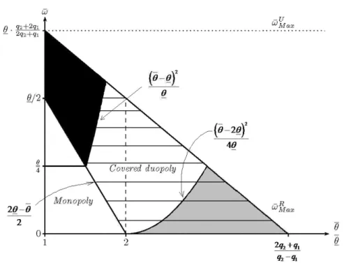
The label is always desirable for the high quality firm, but may be profitable for the low quality firm too. The label helps high qualityfirm to expand its market and to reap a larger part of the quality premium producers are willing to pay. A more interesting result arises when the willingness to pay differ widely across consumers. By revealing true quality of the product 1, the label forces thefirm 1to lower its price. However, when the degree of consumers heterogeneity is high ¡θ >2θ¢, the firm 2 finds optimal to define a high price and to cater to a small market share of producers with high-willingness to pay. Firm 2 acts as a puppy-dog (see Fundenberg and Tirole, 1994), and firm 1 increases its price (see lemma 1). Forω < (θ−_4θ2θ)2, the raising of price is such that the profit of firm 1 is greater with the label.

The grey zone in the figure 2 represents the parameters value for which the labelling benefits to the low quality. Remind that we focus here on cases where the market is covered (ω < ωR

M ax) 13 and both upstream firms produces positive quantities at the equilibrium (ω >max¡0,¡2θ₋θ¢/2¢).

Figure 2: The partition of regulated equilibrium when q1 = 1and q2 = 2.5.

We now investigate the impact of the regulation on the profit of the producers. Pro-ducers are distributed in three categories depending on their quality choice before or after regulation : low-ω producers (ω _∈[0, ωU₁₂]) always choose the high quality product, intermediate-ω producers (ω _∈ [ωU₁₂, ωR₁₂]) switch from the low to the high quality prod-uct with regulation, and high-ω producers (ω _∈ [ωR₁₂, ω]) always choose the low quality product.

Lemma 3 The profit variation of the producer from the regulation is non increasing in

ω. Regulation leads to a decrease of the profit of all the producers if they are not

hetero-1 3

When ω > ωRM ax the regulated market is not covered or covered with firm 1 quoting the price

(r1= (θ−ω)q1)which is just sufficient to cover the market (see Gabszewicz and Thisse,1979, Shaked and Sutton,1982and Wauthy,1996).

geneous enough (ω < (θ−_θθ)2). Otherwise, only the high quality producers with low enough production cost (ω < ωR₁₂₋θ−₃θ) benefit from the regulation.

Proof. See Appendix2.

The lemma 3 states that the producers with the lowest ω are those who benefit the most from the regulation. Consider first the producers who choose the same quality (either low or high) before or after regulation. Their profit variation depends only on the output and input prices. The high quality producers benefit from an output price increase (pR_{2 −}pU > pR_{1 −}pU) but they experience higher input price compared to the low quality producers (r₂R₋rU₂ > r₁R₋r₁U). When the two effects are aggregated, it can easily be shown that the output price effect dominates the input price effect, so that the profit variation of the high quality producer is greater. Consider now the intermediate category of producers who switch from the low to the high quality. Their profit variation is decreasing inωand bounded between the profit variation of high quality producers (low

ω) and the profit variation of the low quality producers (high ω).

The second part of the lemma3concerns the sign of the profit variation. The profit of the producers that keep on selling the low quality with the regulation is decreasing. The price of their product is lower because the low quality of their product is recognized, and this loss is never compensated by the (possible) gain from a decrease of the input price. This result is coherent with the literature on labelling. More interestingly, the lemma 3 also states that the profit of the high quality producer may decreases. By increasing high quality downstream price, the label is considered to benefit to high quality producers (pR

2 −pU >0). But, labelling increases also the high quality upstream price (rR2 −rU2 > 0). So for ω < (θ−_θθ)2 these high quality producers experience a profit loss. As these producers are also those who benefit the most from regulation, we conclude that all the producers loose from regulation under this condition (the cross-hatched zone in figure 2). Conversely, if ω _≥ (θ−_θθ)2, all the producers who keep on producing the high quality benefit from labelling as well as part of those who switch from the low to the high quality (ω _∈hωU₁₂, ωR₁₂₋θ−₃θi).

among the suppliers.

Proposition 1 In scenario A, the regulation benefits to the high quality supply chain (firms and producers) to the detriment of the low quality supply chain ifω > (θ−_θθ)2.

Proof. This proposition is derived from the lemmata2and 3.

This proposition is an intuitive and expected outcome: as regulation reveals the true product quality to the consumer, it benefits to the high quality suppliers to the detriment of the low quality suppliers. The condition on the parameters correspond to the black zone of thefigure2. Note simply that, as we observed just before, the regulation decreases the profit of a fraction of producers that switch to the high quality.

Proposition 2 In scenario A, the regulation benefits to all the upstream firms (low and high quality) to the detriment of all the producers if ω < (θ−_4θ2θ)2.

Proof. This proposition is derived from the lemmata2and 3.

Compared to the proposition 1, the impact of regulation on the suppliers no longer depends on the quality they produce but also their level in the supply chain. Regulation enables the upstream oligopoly to extract more rent from the intermediary producers. Regulation soften price competition between upstreamfirms by enlarging the downstream heterogeneity: product are not only differentiated at the producer level but also at the consumer level. When the consumers’ taste are heterogeneous enough, this effect on upstream competition dominates the quality revelation effect described in the proposition 1.

We may note that forω_∈h(θ−_4θθ)2,(θ−_θ2θ)2i, only the upstream high qualityfirm benefits from the regulation.

Lemma 4 The regulation leads to an increase of the high quality consumer surplus and a decrease of the low quality consumer surplus. Regulation increases the overall consumer surplus and total welfare.

Proof. See Appendix3.

The surplus variation of the consumer who buy the product i with regulation is de-composed as an effect from the variation of the quality (θ(qi−qe)) and an effect from the variation of prices (pR_{i −}pU). The quality effect dominates the price effect so that low quality consumers looses from regulation and high quality consumers benefits from it.

5

The impact of the regulation with low prices equilibrium

on the downstream market (B)

Wefirst consider the stage1equilibrium. As we observed in the section3, the equilibrium

on the downstream market does not affect the demand on the upstream market both

without regulation (equation 1) and with regulation (equation 4). Consequently, the input prices and quantities at the stage 1 equilibrium established in the previous section (equations 6, 7, 9 and 11) are valid in the scenario B. The property concerning the impact of the regulation on the prices, quantities and upstream firms profits (lemmata 1 and 2) are also valid here.

The quality chosen by any intermediary producer or any final consumer is the same in the two scenario A and B. Consequently, the total surplus with or without regulation are identical. Finally, the only difference between these two scenario concerns the output price and the surplus sharing between the intermediary producers and the final consumers.

The equilibrium output price with no regulation is :

pU = 1

3(q1+ 2q2)ω (12)

and, with regulation, is :

pR₁ = (q2−q1) (θ−2(θ−ω)) 3 +q1ω and p R 2 =pR1 + (q2−q1) (θ 2 + 2θω₋θ(θ₋ω)) 3(θ₋θ+ω) (13) Lemma 5 (pR_{1 −}pU)_|A<(pR1 −pU)|B and(pR2 −pU)|A<(pR2 −pU)|B

Proof. (pR

1 −pU)|A−(pR1 −pU)|B = (pR2 −pU)|A−(pR2 −pU)|B=

(q1−q2)(θ−θ)

3 <0 Compared to the scenario A, the price decrease of the low quality good is smaller and the price increase of the high quality good is greater. In other words, with reference to the price of the undifferentiated product, the prices of the differentiated products with regulation are higher in the scenario B compared to the scenario A.

Lemma 6 The profit variation of the producer from the regulation is non increasing in

ω. The low quality producer profit is not affected by the regulation and every high quality producer benefits from regulation. The regulation leads to a decrease of the surplus of all consumers.

Proof. See Appendix4.

It is interesting first to compare this result with those obtained with the scenario A (lemmata 3 and 4). Remind that the profit variation from one scenario to the other corresponds to a transfer between the producers and the consumers. As we observed that the regulation leads to higher prices with the scenario B, it can easily be understood that the regulation is more favorable to the producers (and less to consumers) in this scenario. As we show in the scenario A (lemma 3), the producers with the lowest ω are those who benefit the most from the regulation. Interestingly, the profit of the low quality producer is not affected by the regulation in this scenario B. Remind that prices are defined here so that the participation constraint of the producer with the highest ω is binding (pU _=rU

1 +ωq1 and pR1 =rR1 +ωq1). As a consequence, any variation of the low quality input price is directly transmitted to low quality output price, so that the markup of the low quality producer is not affected by the regulation. All the other producers (with lower ω) necessarily benefit from the regulation, as the profit variation is non increasing inω.

Proposition 3 In scenario B, the regulation is profitable (or not worse of ) for all firms and producers to the detriment of consumers if ω < (θ−_4θ2θ)2. Otherwise, the regulation is profitable only to the high quality suppliers (firm and producer).

Proof. See Lemma2 and6.

When the two upstream firms benefit from the regulation, we observed before (propo-sition 2) that it was detrimental to all the producers in the scenario A. With the same condition, we observe here that it is detrimental to all the consumers in the scenario B. In summary, the scenario does not affect the condition under which the firm extract more rent from the downstream actors, but it affects the actor who is subject to this rent ex-traction. The profit of the producer is higher in the scenario A with no regulation, but the regulation is less beneficial to them compared to the scenario B. Conversely, the consumer surplus is higher in the scenario B with no regulation, but the regulation is less beneficial to them compared to the scenario A.

6

Conclusions

In this paper, we consider a supply chain with two vertically related markets: a competitive downstream market which is supplied by an upstream duopoly. The input purchased in the upstream market is either of high or low quality, its quality determining also that of the output in the downstream market. We assume that while downstream producers are perfectly aware of the quality of the input they purchase, consumers cannot distinguish high from low quality even after consumption. We show that, as expected the regulation may benefit to the high quality supply chain (firms and producers) to the detriment of the low quality supply chain. But more interestingly, we show that downstream labelling may benefit to both upstreamfirms to the detriment to all downstream producers or consumers. So, under labelling, upstreamfirms may extract more rent from the downstream actors.

References

Bonroy O. and Constantatos C. (2008). On the Use of Labels in Credence Goods

Markets. Journal of Regulatory Economics, 33(3), 237-252.

Boom A.(1995). Asymmetric International Minimum Quality Standards and Vertical

Differentiation. Journal of Industrial Economics,43(1), 101-119.

Crampes C. and Hollander A. (1995). Duopoly and Quality Standards. European

Economic Review,39(1), 71-82.

Darby, M., and E. Karni, E. (1973). Free Competition and the Optimal Amount of

Fraud. Journal of Law and Economics,16(1), 67-88.

Fudenberg, D., & J. Tirole, J. (1984). The Fat Cat Effect, the Puppy Dog Ploy and the Lean and Hungry Look. American Economic Review, Paper and Proceeding, 74(2), 361-368.

Fulton, M., and Giannakas, K. (2004). Inserting GM Products into the Food Chain: The Market and Welfare Effects of Different Labeling and Regulatory Regimes. American Journal of Agricultural Economics,86(1), 42-60.

Gabszewicz, J. and Thisse, J. (1979). Price competition, quality and income dispari-ties. Journal of Economics Theory,20, 340-359.

Garella, P. G., and Petrakis, E.(2008). Minimum Quality Standards and Consumers’ Information. Economic Theory,36(2), 283-302.

Hamilton, S. F., and Zilberman, D. (2006). Green Markets, Eco-certification, and Equilibrium Fraud. Journal of Environmental Economics and Management,52, 627-644.

Lapan, H., and Moschini, G. (2007). Grading, Minimum Quality Standards, and the

Labeling of Genetically Modified Products. American Journal of Agricultural Economics,

89(3), 769-783.

Marette, S. (2007). Minimum Safety Standard, Consumers’ Information and

Compe-tition. Journal of Regulatory Economics,32(3), 259-285.

Nelson, P. (1970). Information and Consumer Behaviour. Journal of Political Econ-omy,78(2), 311-329.

Roe, R., and Sheldon, I. (2007). Credence Good Labeling: The Efficiency and Dis-tributional Implications of Several Policy Approaches. American Journal of Agricultural

Economics,89(4), 1020-1033.

Shaked, A. and Sutton, J. (1982). Relaxing Price Competition through Product Dif-ferenciation. Review of Economic Studies,49(1), 3-13.

Tirole, J. (1988). The Theory of Industrial Organisation. Cambridge, Mass: Harvard University Press.

Wang, X. H. and Yang, B. Z.(2001), Mixed-Strategy Equilibria in a Quality Diff eren-tiation Model. International Journal of Industrial Organization,19(1-2), 213-226.

Wauthy, X. (1996). Quality Choice in Models of Vertical Differentiation. Journal of Industrial Economics,44(3), 345-353.

Appendix

Appendix 1: Proof Lemma2.

As we assume that the market is covered before and after the label,ω is restricted to lie in the interval

h M ax(0,2θ₂−θ), ωR_{M ax} i . (2q2+q1)θ−(q2−q1)θ 2q2+q1 ≡ω R M ax < (q2+2q1)θ 2q2+q1 ≡ω U M ax is always true.

1. The impact of label on thefirm2profit is given byπR₂₋πU₂ = 1₉(q2−q1)

³ θ ³ 4θ−3(θ−ω) θ−θ+ω ´ −θ ´ , as4θ₋3 (θ₋ω)> θ₋θ+ω thenπR_{2 −}πU₂ >0,

2. The impact of label on the firm 1profit is given byπR

1 −πU1 =

(q2−q1)((θ−2θ)2−4θω)

9(θ−θ+ω) , then πR_{1 −}πU₁ > 0 when ω _∈ hM ax³0,2θ₂−θ´,(θ−_4θ2θ)2i and πR_{1 −}πU₁ < 0 when

ω_∈h(θ−_4θ2θ)2, ωR_{M ax}i. We may note that the intervalhM ax³0,2θ₂−θ´,(θ−_4θ2θ)2iexists if and only ifθ >2θ (i.e. (θ−_4θ2θ)2 > 2θ₂−θ), soθ >2θis a necessary condition to have

πR_{1 −}πU₁ >0.

Appendix 2: Proof Lemma3.

Remind that ωU₁₂=ω₃ andωR₁₂= (2θ−θ+ω)ω

3(θ−θ+ω) . The producers population may be decom-posed in three groups:

1. Producers defined by ω _∈ £0, ωU₁₂¤ supply high quality output both without and with regulation. The regulation leads to the following profit variation ¡pR_{2 −}rR₂¢₋ ¡

pU₋rU₂¢= (q2−q1)(θω−(θ−θ)

2₎

3(θ−θ+ω) . This profit variation does not depend on ω and is consequenlty non increasing inω. This profit variation is negative isω_∈

h M ax ³ 0,2θ₂−θ ´ ,(θ−_θθ)2 i , and positive ifω _∈h(θ−_θθ)2, ωR_{M ax}i. 2. Producers defined by ω _∈ £ωU 12, ωR12 ¤

switch from the low to the high quality be-cause of the regulation. Their profit variation from the regulation is given by

¡ pR 2 −r2R−ωq2 ¢ −¡pU _−rU 1 −ωq1 ¢ = (q2−q1)(ω 2_{+θω−(θ−θ)}2₎ 3(θ−θ+ω) −ω(q2−q1). This profit variation is decreasing in ω, positive for ω _∈ hωU₁₂, ωR₁₂₋θ−₃θi and negative for

ω_∈hωR₁₂₋θ−₃θ, ωR₁₂i.Note that the profit variation is always negative for all these producer if ω_∈hM ax³0,2θ₂−θ´,(θ−_θθ)2ibecause we then have ωR₁₂₋θ−₃θ < ωU₁₂.

3. Producers defined by ω _∈ £ωR 12, ω

¤

supply high quality output both without and with regulation. The impact of the regulation on their profit is given by¡pR_{1 −}rR₁¢₋ ¡

pU_−rU 1

¢

= ₋1₃(q2−q1) (θ−θ) <0. This profit variation does not depend on ω and is consequenlty non increasing inω.

Appendix 3: Proof Lemma4.

- Impact of the regulation on the consumers surplus. In the unregulated market con-sumer surplus is given by: SCU = 1

θ−θ

Rθ

θ(θqe−p U_)dθ.

In the regulated market we have : SCR=SC₁R+SC₂R withSC₁R= 1 θ−θ RpR₂−pR₁ q2−q1 θ (θq1− pR₁)dθ and SC₂R= 1 θ−θ Rθ pR₂−pR₁ q2−q1 (θq2−pR2)dθ.

• The impact of regulation on the low quality consumer surplus is given by : SC₁R₋

1 θ−θ RpR₂−pR₁ q₂−q₁ θ (θqe−pU)dθ= (q1−q2)(θ−θ)(θ−2θ+2ω) 2 54(θ−θ+ω)2 <0

• The impact of regulation on the high quality consumer surplus is given by : SC₂R₋

1 θ−θ Rθ pR 2−pR1 q₂−q₁ (θqe−pU)dθ= (q2−q1)(θ−θ)(θ+θ−ω)(2θ−θ+ω) 27(θ−θ+ω)2 >0

• The impact of regulation on the total consumer surplus, given by SCR_{, is positive} if and only if³θ2+ 2θ(θ₋ω)₋2(θ₋ω)2´>0this condition is always respected in a duopoly equilbrium.

- Impact of the regulation on the total welfare. Using the footnote11, we may defined welfare social in the regulated market byWR= 1

λ−λ Ã RrR₂−rR₁ q₂−q₁ λ (λq1)dλ + Rλ rR₂−rR₁ q₂−q₁ (λq2)dλ ! withλ=θ₋ω and λ=θ₋ω.

In the unregulated market, welfare social is given by WU = SCU +ΠU with ΠU = 1 ω−ω ³RωU 12 ω (pU−ωq2)dω + Rω ωU 12(p U_−ωq 1)dω ´ . As WR₋WU = (q2−q1)5θ 2 −2θθ−2θω+2θ2

Appendix 4: Proof Lemma5.

As in the appendix 2, producers are distributed in three categories. (1) Producers, defined by ω _∈£0, ωU

12

¤

, supply high quality output before and after the regulation. The impact of the regulation on their profit is given by¡pR_{2 −}r₂R¢₋¡pU₋rU₂¢= (q2−q1)θω

3(θ−θ+ω) >0. (2) Producers, defined by ω _∈ £ωR

12, ω

¤

, supply low quality output before and after the regulation, the impact of the label on their profit is given by ¡pR_{1 −}rR₁¢₋¡pU₋rU₁¢= 0. (3) The profit of any producer who switch from low to high quality product (defined by

ω_∈£ωU₁₂, ωR₁₂¤) is necessarily positive, because he would otherwise keep on producing the low quality.

Note that the profit variation is non increasing inωbecause it is independant fromωin thefirst and the third category and because ∂((p

R

2−r2R−ωq2)−(pU−rU1−ωq1))

∂ω =−(q2−q1)<0

for the second category ( ω_∈£ωU₁₂, ωR₁₂¤).

The impact of regulation on the low quality consumer surplus is given by :

SC₁R₋ 1 θ₋θ Z pR₂−pR₁ q₂−q₁ θ (θqe−pU)dθ= (q1−q2) (θ−θ) ¡ θ₋2θ+ 2ω¢ ¡7θ₋8θ+ 8ω¢ 54(θ₋θ+ω)2 <0

The impact of regulation on the high quality consumer surplus is given by :

SC₂R₋ 1 θ₋θ Z θ pR 2−pR1 q₂−q₁ (θqe−pU)dθ= 2 (q1−q2) (θ−θ) ¡ θ₋2θ+ 2ω¢ ¡2θ₋θ+ω¢ 27(θ₋θ+ω)2 <0