Durham Research Online
Deposited in DRO:31 March 2014
Version of attached le:
Accepted Version
Peer-review status of attached le:
Peer-reviewed
Citation for published item:
Coolen-Maturi, T. and Coolen, F.P.A. (2011) 'Unobserved, re-dened, unknown or removed failure modes in competing risks.', Proceedings of the Institution of Mechanical Engineers, part O : journal of risk and reliability., 225 (4). pp. 461-474.
Further information on publisher's website: http://dx.doi.org/10.1177/1748006X11401706
Publisher's copyright statement:
The nal denitive version of this article has been published in the journal Proceedings of the Institution of Mechanical Engineers, Part O: Journal of Risk and Reliability, 225 (4) 2011 cInstitution of Mechanical Engineers by SAGE Publications Ltd at the Proceedings of the Institution of Mechanical Engineers, Part O: Journal of Risk and Reliability page: http://pio.sagepub.com/content/225/4/461 on SAGE Journals Online: http://online.sagepub.com/
Additional information:
Use policy
The full-text may be used and/or reproduced, and given to third parties in any format or medium, without prior permission or charge, for personal research or study, educational, or not-for-prot purposes provided that:
• a full bibliographic reference is made to the original source • alinkis made to the metadata record in DRO
• the full-text is not changed in any way
The full-text must not be sold in any format or medium without the formal permission of the copyright holders. Please consult thefull DRO policyfor further details.
Durham University Library, Stockton Road, Durham DH1 3LY, United Kingdom Tel : +44 (0)191 334 3042 | Fax : +44 (0)191 334 2971
Unobserved, re-defined, unknown or removed
failure modes in competing risks
Tahani Coolen-Maturi
∗Frank P.A. Coolen
†Department of Mathematical Sciences
Durham University, Durham DH1 3LE, UK
Abstract
Recently the nonparametric predictive approach to inference for competing risks was introduced [1]. In this paper further results for such inferences are presented, with focus on four important and closely related aspects. First, the effect of defined failure modes which thus far have not yet caused failures is studied. Secondly, the effect of re-defining (groups of) failure modes is considered, followed by a discussion of possible unknown, so undefined, failure modes. Finally, the effect of removal of failure modes is illustrated.
Key words: competing risks; failure modes; lower and upper probabilities; lower and upper survival functions; nonparametric predictive inference; right-censored data.
1
Introduction
Maturi et al [1] presented nonparametric predictive inference (NPI) for competing risks, considering prediction of the failure time of a future unit which is exchangeable with the units observed and with specific attention to prediction of the failure mode that will cause this unit to fail. In NPI [2, 3] lower and upper probabilities (also known as imprecise probability [4] or interval probability [5]) are used to quantify uncertainty, which enables the use of relatively few modelling assumptions and hence inferences which are strongly based on observed data. In this paper further results for such inferences are presented, with focus on four important and closely related aspects. First, the effect of defined failure modes which thus far have not yet caused failures is studied. As these have not yet been observed, there is no empirical evidence in favour of the event that they will, or even can, cause the next unit to fail, but of course any finite amount of data can also not logically exclude the
∗Email address: [email protected]
possibility that such a failure mode might cause the next unit’s failure. The use of lower and upper probabilities is well suited to reflect this, and for several situations explicit formulae for the NPI lower and upper probabilities are presented and discussed. Secondly, the effect of re-defining failure modes, by grouping some of them into a single new failure mode, is analyzed. Such re-defining of failure modes affects the NPI lower probabilities, and the number of failure modes used for a given data set dictates the total amount of imprecision. Thirdly, possible unknown, so undefined, failure modes are discussed. Classical statistical methods that use precise probability for uncertainty quantification typically struggle to deal with such possible undefined failure modes, the NPI method can deal with such failure modes in a way that links logically to defined but unobserved failure modes. Finally, the removal of failure modes is considered, with focus on the effect on the NPI lower and upper survival functions for the failure time of the next unit when removing a specific failure mode, which provides useful input into a possible decision about which failure mode to remove.
This paper considers competing risks with as starting point k distinct defined failure modes that can cause a unit to fail and that occur independently, with some variations when the effects of unknown failure modes or of removing a failure mode are considered. First, an overview of the results of [1] is given in Section 2, for more information about competing risks and the related literature the reader is referred to [1]. This is followed by further analysis and discussion of the effects of unobserved, re-defined, unknown or removed failure modes in Sections 3, 4, 5 and 6, respectively. The results are illustrated and further discussed in an example in Section 7, followed by some brief concluding remarks in Section 8. The paper ends with several appendices which contain the proofs of results in the paper and an overview of notation.
2
NPI for competing risks
Nonparametric predictive inference (NPI) is a statistical method based on Hill’s assumption
A(n)[6], which gives a direct conditional probability for a future observable random quantity,
given observed values of related random quantities [2, 3]. Let Y1, . . . , Yn, Yn+1 be positive,
continuous and exchangeable random quantities representing event times. Suppose that the values of Y1, . . . , Yn are observed and the corresponding ordered observed values are
denoted by 0 < y1 < . . . < yn < ∞, for ease of notation let y0 = 0 and yn+1 = ∞.
For ease of presentation, it is assumed that no ties occur among the observed values. It is quite straightforward to deal with tied observations in this setting, by assuming that tied observations differ by small amounts which tend to zero. For the random quantity
Yn+1 representing a future observation, based on n observations, the assumption A(n) [6] is
P(Yn+1 ∈(yi−1, yi)) = 1/(n+ 1) fori= 1, . . . , n+ 1. A(n) does not assume anything else, and
can be interpreted as a post-data assumption related to exchangeability [7]. Inferences based onA(n) are predictive and nonparametric, and can be considered suitable if there is hardly
any knowledge about the random quantity of interest, other than the n observations, or if one does not want to use such information, e.g. to study effects of additional assumptions underlying other statistical methods. A(n) is not sufficient to derive precise probabilities
for many events of interest, but it provides bounds for probabilities via the ‘fundamental theorem of probability’ [7], which are lower and upper probabilities in interval probability theory [2, 4, 5].
In reliability analyses, data on event times are often affected by right-censoring, where for a unit it is only known that the event has not yet taken place at a specific time. Coolen and Yan [8] presented a generalization of A(n), called ’right-censoring A(n)’ or rc-A(n), which
is suitable for NPI with right-censored data and uses the additional assumption that, at the moment of censoring, the residual lifetime of a right-censored unit is exchangeable with the residual lifetimes of all other units that have not yet failed or been censored. To formulate the required form of rc-A(n)for NPI with competing risks the concept of M-functions is used
[8]. AnM-function provides a partial specification of a probability distribution and is math-ematically equivalent to Shafer’s ‘basic probability assignments’ [9]. It assigns probability masses to intervals, which may be overlapping, without making any assumption about the distribution of the probability mass assigned to such an interval, and with the sum of all such probability masses equal to one.
Suppose that there are n observations consisting of u failure times, x1 < x2 < . . . < xu,
and n − u right-censored observations, c1 < c2 < . . . < cn−u. Let x0 = 0 and xu+1 =
∞. Suppose further that there are si right-censored observations in the interval (xi, xi+1),
denoted by ci
1 < ci2 < . . . < cisi, so
Pu
i=0si = n −u. The assumption rc-A(n) [8] partially
specifies the NPI probability distribution for Xn+1, the failure time of one future unit, by
the following M-function values, for i= 0,1, . . . , u and i∗ = 0,1, . . . , s
i, MXn+1(t i i∗, xi+1)= 1 (n+1)(˜ntii∗) δi i∗−1 Y {r:cr<tii∗} ˜ ncr+1 ˜ ncr (1) where δi i∗ = ( 1 if i∗ = 0 i.e. ti
0 =xi (failure time or time 0)
0 if i∗ = 1, . . . , s
i i.e. tii∗ =cii∗ (censoring time)
and ˜ncr and ˜ntii∗ are the number of units in the risk set just prior to time cr and t
i
i∗,
respec-tively, with the definition ˜n0 =n+ 1 for ease of notation. Only intervals of this form have
positive M-function values, and these sum up to one over all these intervals. Summing up all M-function values assigned to such intervals with the same xi+1 as right endpoint gives
the probability P(Xn+1 ∈(xi, xi+1)) = 1 n+ 1 Y {r:cr<xi+1} ˜ ncr + 1 ˜ ncr (2)
where xi and xi+1 are two consecutive failure times (and x0 = 0, xu+1 =∞). It should be
In addition to notation introduced above, let ti
si+1 =t
i+1
0 = xi+1 for i = 0,1, . . . , u−1.
The NPI lower and upper survival functions for the failure time Xn+1 of the next unit are
denoted by S(t) and S(t), respectively, and are as follows [1, 10]. For t ∈ [ti
a, tia+1) with i= 0,1, . . . , u and a= 0,1, . . . , si, S(t) = 1 n+ 1 ˜ntia Y {r:cr<tia} ˜ ncr + 1 ˜ ncr (3)
and for t∈[xi, xi+1) with i= 0,1, . . . , u,
S(t) = 1 n+ 1 n˜xi Y {r:cr<xi} ˜ ncr + 1 ˜ ncr (4)
In NPI for competing risks [1], it is assumed that there are k defined failure modes and a unit fails due to the first occurrence of a failure mode, which is identified with certainty. Let Xn+1 denote the failure time of a future unit, and let the corresponding notation for
the failure time including indication of the actual failure modej be Xj,n+1. As the different
failure modes are assumed to occur independently, the competing risk data per failure mode consist of a number of observed failure times for failures caused by the specific failure mode considered, and right-censoring times for failures caused by other failure modes. Hence
rc-A(n) can be applied per failure mode j for inference on Xj,n+1. Suppose that uj failures are
caused by failure mode j, at timesxj,1 < xj,2 < . . . , < xj,uj, and let n−uj be the number of
the right-censored observations, cj,1 < cj,2 < . . . < cj,n−uj, corresponding to failure mode j.
For notational convenience, letxj,0 = 0 andxj,uj+1 =∞. Suppose further that there are sj,ij
right-censored observations in the interval (xj,ij, xj,ij+1), denoted byc
ij j,1 < c ij j,2 < . . . < c ij j,sj,ij, so Puj
ij=0sj,ij = n −uj. It should be emphasized that it is not assumed that each unit
considered must actually fail, if a unit does not fail then there will be a right-censored observation recorded for this unit for each failure mode, as it is assumed that the unit will then be withdrawn from the study, or the study ends, at some point. The random quantity representing the failure time of the next unit, with all k failure modes considered, isXn+1 = min
1≤j≤kXj,n+1.
The NPI M-functions for Xj,n+1 (j = 1, . . . , k), similar to (1), are
Mj(tij j,i∗ j, xj,ij+1) =MXj,n+1(t ij j,i∗ j, xj,ij+1) = 1 (n+ 1)(˜ntijj,i∗ j )δ ij i∗ j −1 Y {r:cj,r<tijj,i∗ j } ˜ ncj,r + 1 ˜ ncj,r (5)
where ij = 0,1, . . . , uj, i∗j = 0,1, . . . , sj,ij and
δij i∗ j = ( 1 if i∗j = 0 i.e. t ij
j,0 =xj,ij (failure time or time 0)
0 if i∗j = 1, . . . , sj,ij i.e. t ij j,i∗ j =c ij j,i∗ j (censoring time)
Again ˜ncr and ˜ntij j,i∗
j
are the numbers of units in the risk set just prior to times cr and t
ij
j,i∗
j,
respectively. The corresponding NPI probabilities, similar to (2), are
Pj(x
j,ij, xj,ij+1) = P(Xj,n+1 ∈(xj,ij, xj,ij+1)) =
1 n+ 1 Y {r:cj,r<xj,ij+1} ˜ ncj,r + 1 ˜ ncj,r (6)
where xj,ij and xj,ij+1 are two consecutive observed failure times caused by failure mode j
(and xj,0 = 0, xj,uj+1 = ∞). The corresponding NPI lower and upper survival functions
for Xj,n+1 are denoted by Sj and S
j
, respectively, and are similar to the lower and upper survival functions S and S given in equations (3) and (4) but with an additional subscript
j added to all notations to indicate the specific failure mode.
A special case considered several times in this paper is where one failure mode, say failure mode O, causes all the observed failures. In this case, the NPI M-functions for XO,n+1 as
given by (5) are identical to those given by (1), hence also SO(t) = S(t) and SO(t) = S(t) for all t≥0.
Consider the event that a single future unit, called the ’next unit’, undergoing the same test or process as the n units for which failure data are available, fails due to failure mode
l. The NPI lower and upper probabilities for this event are
P(l) = XXX C(j, ij, i∗j) " u l X il=0 1(xl,il+1 < min 1≤j≤k j6=l {tij j,i∗ j})×P l (xl,il, xl,il+1) # k Y j=1 j6=l Mj(tij j,i∗ j, xj,ij+1) (7) P (l)= XXX C(j, ij) " ul X il=0 sl,il X i∗ l=0 1(til l,i∗ l <1min≤j≤k j6=l {xj,ij+1})×M l (til l,i∗ l, xl,il+1) # k Y j=1 j6=l Pj(xj,ij, xj,ij+1) (8) where XXX C(j, ij, i∗j)
denotes the sums over all i∗
j from 0 to sj,ij and over all ij from 0 to uj for
j = 1, . . . , k but not including j =l. Similarly, XXX
C(j, ij)
denotes the sums over all ij from 0 to
uj for j = 1, . . . , k but not includingj =l.
3
Unobserved failure modes
One or more of the k defined failure modes may not have led to any failures of the n units. In this case all observed failure times are right-censored observations when considering such unobserved failure modes. To study the effect of unobserved failure modes, the situation where all n observed units have actually failed, each due to one of the k failure modes, is considered first.
For any unobserved failure mode U ∈ {1, . . . , k}, the NPI lower and upper probabilities for the event that the next unit will fail due to U are
P(U) = 0 (9) P(U) = 1 n+ 1 n+1 X i=1 1 i (10)
Since all observed event times for then units are right-censored times with respect to failure mode U, the NPI lower probability (9) follows immediately from (7), and the fact that it is equal to zero reflects that no failures caused by failure mode U have been observed, so it cannot be excluded that failure mode U might never actually cause a failure. The proof of the NPI upper probability (10) is given in Appendix B. This upper probability is decreasing inn with limit 0 ifn→ ∞, which is in line with intuition as the evidence against a specific unobserved failure mode causing the next unit to fail decreases with increasing numbers of observed failures which are all caused by other failure modes. It is important to emphasize that this upper probability holds for each defined but unobserved failure mode, no matter how many of the k defined failure modes are unobserved. This inference shows strong advantages of the use of lower and upper probabilities in risk analyses. The lower probability with value 0 implies that it cannot be excluded that an unobserved failure mode indeed will not occur, but it still can occur as reflected by the positive upper probability. The sub-additivity of upper probabilities [4, 5] allows a meaningful positive value independent of the number of specified unobserved failure modes. Both these advantages are not available when using precise probabilities but are important in risk analysis, in particular when there is relatively limited information.
One extreme situation with k defined failure modes that may occur is if alln units failed due to a single one of these failure modes, hence leaving k −1 failure modes unobserved. In this case, the NPI lower and upper probabilities for the event that the next unit will fail due to any specific one of these unobserved failure modes are again as given by (9) and (10). For the one failure mode which caused all n observed failures, say failure mode O, the NPI lower and upper probabilities for the event that the next unit will fail also due to this failure mode are P(O)= 1 n+ 1 n X i=1 i i+ 1 k−1 (11) P(O)= 1 (12)
The fact that the upper probability (12) is equal to one is logical as it cannot be excluded on the basis of the data only that there would never be any failures caused by another failure mode than O. The lower probability (11) follows from (7), as shown in Appendix C. For
k = 2 the lower probability (11) is equal to P(O)= 1 n+ 1 n X i=1 i i+ 1 = 1− 1 n+ 1 n+1 X i=1 1 i (13)
which also follows from (10) and the conjugacy property P(A) = 1−P(Ac), for any event
A and its complementary event Ac, which holds for all NPI lower and upper probabilities
presented in this paper [2, 4, 5].
An important generalization of the situation discussed above is considered next, again with k defined failure modes but now allowing n−u units not to fail due to any of the k
defined failure modes (they may e.g. be censored due to being removed from the study, but this censoring process is assumed to be independent of the failure processes corresponding to the k defined failure modes), so these units lead to right-censored observations for each failure mode [1]. In this case, the NPI lower and upper probabilities for the event that the next unit fails due to any specific unobserved failure modeU are
P(U)= 0 (14) P(U)= u+1 X i=1 1 ˜ nxi+ 1 2 S(xi−1) (15)
where x1 < x2 < . . . < xu are the u observed failure times regardless which failure modes
caused the failures (other than U, of course), with x0 = 0, xu+1 = ∞ and ˜nxu+1 = 0. The
upper survival function S(.) is as given by (4), so it is the upper survival function for the future unit Xn+1 without taking any notice of the different failure modes. The effect of
the n−u units that did not fail is taken into account through this upper survival function
S(.), which is also equal to the product of the upper survival functions corresponding to the specific failure modes [10]. Foru=n this upper probability (15) is equal to (10). The proof of (15) is given in Appendix B. The lower probability (14) follows again directly from (7) and as for (9) this is an intuitively logical result.
For the situation with one of thek defined failure modes, say failure modeO, causing all the u observed failures, the generalization of the NPI lower probability (11) is
P(O)= n X i=1 S(cn−i)−S(cn+1−i) i i+ 1 k−1 (16)
whereS is the NPI upper survival function (4), which, as mentioned before, is equal in this case to the NPI upper survival function SO for XO,n+1. This lower probability is proven in
Appendix C. The corresponding NPI upper probability is equal to one, so P(O) = 1, with the same intuitive explanation as discussed before.
In the special case with only k = 2 failure modes, with one of these (failure mode O) causing all theu observed failures (and againn−u units not failing due to these two failure
modes) the NPI lower and upper probabilities for the event that the next unit fails also due to failure mode O are
P(O) = 1− u+1 X i=1 1 ˜ nxi+ 1 2 S(xi−1) and P (O) = 1 (17)
These results can be derived either directly or by using (14) and (15) and the conjugacy property.
4
Re-defined failure modes
It may be of interest to re-define the k failure modes by combining some of them into new single failure modes, suppose this leads to s(< k) re-defined failure modes. This situation has been studied in detail for the case where alln units actually failed due to the considered failure modes. A nice fact is that, no matter how thekoriginal failure modes are grouped into these s re-defined failure modes, the sum of thes corresponding NPI lower probabilities for the events that the next unit will fail due to a specific one of these re-defined failure modes, is constant, and also the sum of the corresponding NPI upper probabilities is constant. These sums of lower and upper probabilities are
s X l=1 P (l)=P(O) and s X l=1 P (l)= 1 + (s−1)P(U) (18)
with P(U) and P (O) as given in (10) and (11). The proof of (18) is given in Appendix D. For the situation where some of then units did not fail due to one of the considered failure modes, the equations (18) also appear to hold, with no counter-examples found numerically, but they have not been proven due primarily to complexity of the general forms of the lower and upper probabilities and the notation involved.
The idea of re-grouping the k defined failure modes into s re-defined failure modes also leads to interesting facts for the NPI lower and upper survival functions for the next unit, which actually hold for all situations including the possibility of some of the n units not having failed due to one of the considered failure modes. Due to the assumed independence of the k failure modes, and hence also of the s re-defined failure modes which followed by grouping some of the original failure modes, the NPI lower survival function for the next unit, in case of s (re-defined) failure modes, is (using subscript sCR to emphasize that s
competing risks are used), for t∈[ti
a, tia+1) withi= 0,1, . . . , u and a= 0,1, . . . , si, SsCR(t) = s Y j=1 Sj(t) = ˜ nti a ˜ nti a + 1 s−1 S(t) (19)
where S(t) is the NPI lower survival function (3) corresponding to total neglect of the different failure modes. Similarly, the corresponding NPI upper survival function is, for
t∈[xi, xi+1) with i= 0,1, . . . , u, SsCR(t) = s Y j=1 Sj(t) =S(t) (20)
withS(t) the NPI upper survival function (4) corresponding to total neglect of the different failure modes. Note that these lower and upper survival functions do not depend on the specific grouping of failure modes into s re-defined failure modes, and (19) and (20) also hold for the originally defined failure modes, so with s = k. A direct consequence of (19) and (20) is that if the numbersof re-defined failure modes increases, then the NPI lower sur-vival function decreases while the corresponding upper sursur-vival function remains unchanged, hence the use of more (re-defined) failure modes for the same failure data leads to increased imprecision. This fact was observed and discussed before in examples by Maturi et al. [1]. The proof of (19) and (20) is given in Appendix E.
Finally, it is worth noting that the NPI lower and upper survival functions for the next unit, conditioned on failure due to an unobserved failure modeU, are
SU(t) = n˜tia ˜ nti a + 1 (21) for t∈[ti
a, tia+1) withi= 0,1, . . . , u and a= 0,1, . . . , si, and
SU(t) = 1 (22)
for all t≥ 0. For the other extreme situation, namely if one failure mode O had caused all
u≤nobserved failures, it was already mentioned in Section 2 that the NPI lower and upper survival functions for the next unit, conditioned on failure due to this failure mode O, are justSO(t) =S(t) and SO(t) =S(t), with the NPI lower and upper survival functions on the right-hand sides again given by (3) and (4). Therefore the expressions above also lead to the following equality for the lower survival functions
SsCR(t) = SU(t)s−1
SO(t) (23)
with the similar expression also trivially valid for the corresponding upper survival functions due to equality (22).
5
Unknown failure modes
Thus far the effect of known failure modes has been studied, with particular focus on defined failure modes which have not yet caused any failures (hence being unobserved). But there may be unknown risks, that is failure modes that are possible but that have not been defined or even recognized. It is reasonable to assume that any failure mode that caused one of the
method does not require these failure modes to have been defined before the test data became available. So unknown unobserved failure modes are now considered. An advantage of the theory presented in this paper is that, for any such a failure mode, the NPI lower and upper probabilities for the event that it will cause the next unit to fail are equal to (9) and (10), or (14) and (15) if not all units failed, as these results do not actually depend on the number k of specified failure modes, hence an unknown unobserved failure mode can be considered just as a further defined yet unspecified failure mode. No detailed analysis is presented for multiple unknown unobserved failure modes, as it seems unlikely to be of great practical relevance to go beyond the possible existence of one unknown unobserved failure mode when considering only a single next unit. It may be interesting to do so when considering for example two future units, with interest in the event that they will fail due to two different unknown unobserved failure modes, such questions are left as interesting topics for future research.
Inclusion of an unknown failure mode will decrease the NPI lower probability for the event that another failure mode causes the next failure, if that other failure mode has already caused a failure. However, it will not affect the corresponding upper probability. This is discussed in the example in Section 7. The ability of the NPI approach presented in this paper to deal with unknown unobserved failure modes, in a manner that is in line with intuition and based on the relatively few modelling assumptions, is an attractive feature for practical risk analysis.
This consideration of the possible effect of an unknown failure mode, closely related to an unobserved failure mode, does not include any inference on how likely it is that an unknown or unobserved failure mode actually will occur, which is also a highly relevant inference in risk analysis. An NPI solution to this problem has been presented [11] which uses a model for multinomial data [12], with the NPI lower probability of the next unit failing due to either a specified unobserved or unspecified unobserved failure mode being equal to zero and the corresponding NPI upper probability being positive and depending on the number of failures and on the number of different failure modes observed thus far.
6
Removing failure modes
In practical situations it may be of interest to consider the effect of removal of a failure mode, which for example may be possible by re-designing or repairing a system or investing in units which are resistant to a specific failure mode. There may be a budget enabling removal of one or more failure modes and therefore one may wish to analyse the effect of doing so for the different failure modes. Suppose that there are s failure modes that can cause a unit to fail, withs ≤k used to reflect that these may include re-defined failure modes consisting of groups of thek originally defined failure modes. Of course, unknown failure modes are not included in this discussion, but it may be worth to consider removal of unobserved failure
modes. However, it typically will be most beneficial to remove failure modes that have already caused failures, so in the example in Section 7 focus will be on such failure modes. As the re-defined failure modes result from combinations of some of thek originally defined failure modes, hence this analysis immediately also includes the combined effect of deleting multiple failure modes. It should be emphasized that the data remain unchanged when a failure mode is removed, its effect will just be that this specific failure cannot cause the next unit to fail. The effect of removing a failure mode on the NPI lower and upper survival functions for the next unit is of interest. With s failure modes, these NPI lower and upper survival functions for the failure timeXn+1 = min
1≤j≤s{Xj,n+1} of unit n+ 1 are SsCR(t) = s Y j=1 Sj(t) and SsCR(t) = s Y j=1 Sj(t) (24)
If failure mode i∗ is removed from the competing risks, then the corresponding NPI lower
and upper survival functions are
SsCR∗i(t) = s Y j=1 j6=i∗ Sj(t) and SsCR ∗i (t) = s Y j=1 j6=i∗ Sj(t) (25)
The following relationships hold for different NPI lower and upper survival functions in such a scenario, with as beforeSand S the NPI lower and upper survival functions, as given by (3) and (4), for the next unit in the situation with the information of the failure modes causing particular failures not taken into account. For the lower survival functions,
SsCR(t)≤SsCR∗i(t)≤S(t) (26)
for allt≥0, where the first inequality is trivial (and sharp as long as both sides are positive) and the second inequality follows from (19). Similarly, for the corresponding upper survival functions,
S(t) =SsCR(t)≤SsCR
∗i
(t) (27)
for allt ≥0, where the inequality is again trivial (and sharp except if both sides are equal to one), and now the first relation is an equality which follows from (20). The effect of removal of a failure mode is illustrated, with some further discussion, in the example in Section 7.
7
Example
The topics discussed in this paper are illustrated using data based on a well-known data set from the literature [13]. The original data contain information about 36 units of a new model of a small electrical appliance which were tested, and where the lifetime observation per unit consists of the number of completed cycles of use until the unit failed. There were 18
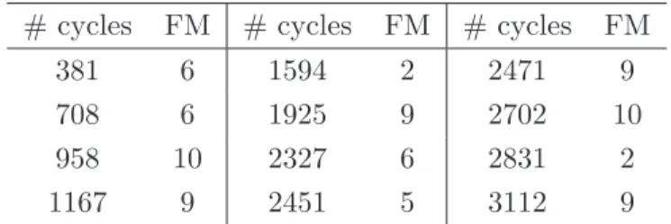
possible failure modes. Maturiet al [1] used this complete data set to illustrate the general NPI method for competing risks. In this paper, to illustrate the specific effects discussed more clearly, a subset of the data is selected, consisting of 12 of the original 36 units. These data are presented in Table 1, which also includes the specific failure mode (FM) that caused the unit to fail.
# cycles FM # cycles FM # cycles FM 381 6 1594 2 2471 9 708 6 1925 9 2702 10 958 10 2327 6 2831 2 1167 9 2451 5 3112 9
Table 1: Failure data for electrical appliances
The two most frequently occurring failure modes in these data are FM9 and FM6, which caused 4 and 3 units to fail, respectively. The event of interest is that the next unit, say unit 13, will fail due to a specific failure mode, assuming it would undergo the same test and its number of completed cycles would be exchangeable with these numbers for the 12 units reported. Twelve cases are presented, (A) to (L), each involving a different grouping of the failure modes in 2, 3 or 4 re-defined failure modes (so s = 2,3,4), the corresponding NPI lower and upper probabilities are presented in Table 2. The term OFM is introduced for ‘other failure modes’ grouped into one single re-defined failure mode. For example in case (A), OFM is considered to be a single new failure mode containing all originally defined failure modes except failure mode 9. For each case the sums of the lower probabilities and of the upper probabilities are also given, these illustrate that they are constant for fixed values of s as presented in Section 4 (with some effects of rounding).
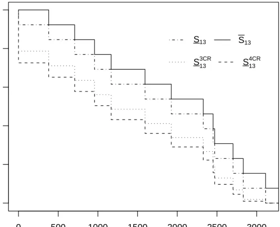
Figure 1 shows the NPI lower and upper survival functions for the failure time X13 of
unit 13 for three situations, for which the upper survival functions are identical hence only the lower survival functions differ. The lower survival function for X13, denoted by S13 in
Figure 1, is as given by (3) and results from total neglect of the information on different failure modes, hence just by applying rc-A(12) [6] with 12 observed failure times. The lower
survival function S313CR corresponds to situations with s = 3 (re-defined) failure modes and
follows from (19), so this is the lower survival function for cases (F)-(H) in Table 2. Similarly, the lower survival functionS413CR corresponds to the situation with s= 4 (re-defined) failure
modes, so cases (I)-(L) in Table 2. By (20) the corresponding upper survival functions are all the same.
These NPI lower survival functions illustrate the general feature of NPI for competing risks, presented in Section 4, that if the number s of re-defined failure modes in which the
k original failure modes are grouped (note that S13 can be interpreted as the case s = 1)
increases, then the corresponding lower survival function decreases, so with unchanged upper survival function this leads to increased imprecision.
P P P P (A) (B) 9 0.2365 0.4812 6 0.2075 0.4521 OFM 0.5188 0.7635 OFM 0.5479 0.7925 0.7553 1.2447 0.7554 1.2446 (C) (D) 10 0.1276 0.3722 2 0.1197 0.3643 OFM 0.6278 0.8724 OFM 0.6357 0.8803 0.7554 1.2446 0.7554 1.2446 (E) (F) 5 0.0641 0.3087 9 0.1897 0.4812 OFM 0.6913 0.9359 6 0.1867 0.4521 OFM 0.2552 0.5560 0.7554 1.2446 0.6316 1.4893 (G) (H) 9 0.1897 0.4812 9 0.1897 0.4812 10 0.1068 0.3722 3 0 0.2446 OFM 0.3351 0.6358 OFM 0.4419 0.7635 0.6316 1.4892 0.6316 1.4893 (I) (J) 9 0.1566 0.4812 9 0.1566 0.4812 6 0.1682 0.4521 6 0.1682 0.4521 10 0.0902 0.3722 3 0 0.2446 OFM 0.1213 0.4284 OFM 0.2116 0.5560 0.5363 1.7339 0.5364 1.7339 (K) (L) 9 0.1566 0.4812 3 0 0.2446 6 0.1682 0.4521 4 0 0.2446 2 0.0768 0.3643 7 0 0.2446 OFM 0.1348 0.4364 OFM 0.5364 1 0.5364 1.7340 0.5364 1.7338
0 500 1000 1500 2000 2500 3000 0.0 0.2 0.4 0.6 0.8 1.0 t Sur viv al function S13 S13 S133CR S134CR
Figure 1: NPI lower and upper survival functions for unit 13; case (I): S413CR, and case (F):
S133CR, and without specified failure modes: S13; note that S134CR =S313CR =S13.
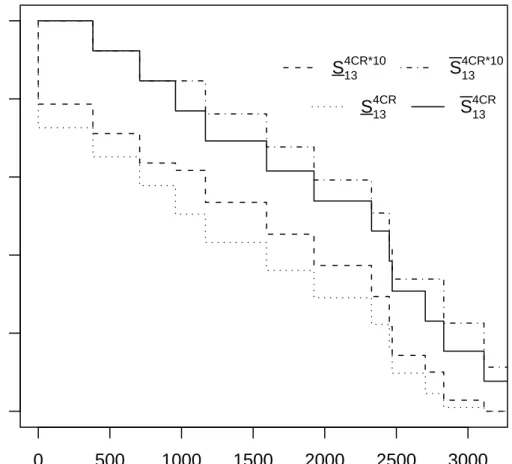
Figure 2 shows the NPI lower and upper survival functions for unit 13 with the failure modes according to case (I) and also the corresponding lower and upper survival functions after failure mode 10 (FM10) has been removed. Of course, removing FM10 has a positive effect on these lower and upper survival functions. It is also interesting to compare case (F), where FM10 is grouped together with OFM, and case (I) but with FM10 removed. Figure 3 presents the NPI lower and upper survival functions for unit 13 for these two cases. It shows that the NPI lower and upper survival functions corresponding to case (I) after removal of FM10 are greater than the NPI lower and upper survival functions corresponding to case (F) when FM10 is taken into account and included in OFM.
In case (A) all failure modes except FM9 are together re-defined as one failure mode (OFM). Suppose that there may be an additional unknown failure mode that may cause the
0 500 1000 1500 2000 2500 3000 0.0 0.2 0.4 0.6 0.8 1.0 t Sur viv al function S134CR*10 S134CR*10 S134CR S134CR
Figure 2: NPI lower and upper survival functions for unit 13, before (S413CR and S413CR) and after (S413CR∗10 and S413CR∗10) removal of FM10 for case (I).
units to fail, but this has not happened for the tested units. To illustrate the effect of such a possible further failure mode, consider case (H) where FM3 has been defined although it had not led to a failure for the tested units. As discussed in Section 5, the effect of such an unknown further failure mode is identical to the effect of a defined unobserved failure mode. The NPI lower and upper probabilities for the event that the next unit fails due to FM3 are 0 and 0.2446 (from (9) and (10)). Including such an unknown failure mode has led to decrease of the lower probabilities for the event that unit 13 will fail due to FM9 or due to OFM, which follows by comparison of cases (A) and (H), while the corresponding upper probabilities are the same in both cases. The same effect is also illustrated by cases (F) and (J), and reflects that the unknown failure mode could possibly lead to the next failure, which would make the other failure modes less likely causes for it, but it cannot be excluded that
0 500 1000 1500 2000 2500 3000 0.0 0.2 0.4 0.6 0.8 1.0 t Sur viv al function S134CR*10 S134CR*10 S133CR S133CR
Figure 3: NPI lower and upper survival functions for unit 13, case (F):S313CR and S313CR, and after removal of FM10 for case (I):S413CR∗10 and S413CR∗10.
this unknown failure mode may not have any effect at all, as reflected by those unchanged upper probabilities.
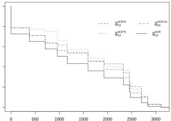
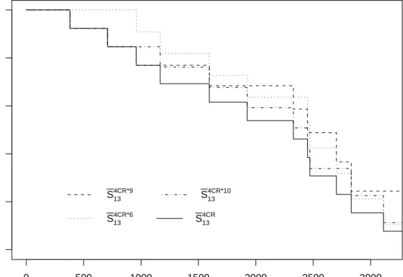
If one has the opportunity to remove a failure mode, the decision which failure mode to remove will probably depend on detailed considerations on costs and the effect of such a removal on the reliability of further units. In the approach presented here, with explicit focus on a single next unit, the effect clearly shows in the changes in the NPI lower and upper survival functions. This effect is illustrated using again case (I) as starting point, so with 4 (re-defined) failure modes. Figures 4 and 5 present the NPI lower and upper survival functions for case (I) and for each of the situations that occur with either FM6, FM9 or FM10 removed. As no single case leads to the best effect, that is no lower or upper survival function dominates the other ones everywhere, further considerations would be required in
0 500 1000 1500 2000 2500 3000 0.0 0.2 0.4 0.6 0.8 1.0 t Sur viv al function S134CR*9 S134CR*10 S134CR*6 S134CR
Figure 4: NPI lower survival functions for case (I): S4CR
13 , and with failure modes 6, 9 or 10
removed: S413CR∗6,S134CR∗9 and S413CR∗10, respectively.
the decision process, for example an explicit goal may be high reliability of the next unit after a specific number of cycles (so generally after a specific moment in time). If there is a particular interest in high reliability for relatively small times t, then removal of FM6 is best, while for larger t it is better to remove FM9 (this shows in both the lower and upper survival functions). This is clearly in line with the data as FM6 caused some of the early failures but FM9 caused more failures over all. The method presented in this paper provides useful information as input in such decision processes, with flexibility to use this information according to specific needs and wishes, and facilitated by the fact that all inferences are explicitly in terms of the next unit considered.
8
Concluding remarks
The results presented in this paper have wide applicability and potential impact, as situa-tions with competing risks occur in many application areas including engineering risk and
0 500 1000 1500 2000 2500 3000 0.0 0.2 0.4 0.6 0.8 1.0 t Sur viv al function S134CR*9 S134CR*10 S134CR*6 S134CR
Figure 5: NPI upper survival functions for case (I):S413CR, and with failure modes 6, 9 or 10 removed: S413CR∗6,S134CR∗9 and S413CR∗10, respectively.
reliability, finance, medical and bio-statistics. A major research challenge for NPI in general is development of appropriate methods to deal with multivariate data, including modelling of dependence and dealing with covariates. Progress on these topics will enable modelling of dependent competing risks and inclusion of covariates, which will widen applicability of this approach. The use of lower and upper probabilities in statistics and related fields has received much attention in the last two decades and has become widely accepted. This pro-vides major research challenges, ranging from detailed understanding of the relation between imprecise probabilities and information to development of models and related computational methods (for more information see www.sipta.organd www.npi-statistics.com).
Appendix A
Lemma 1. In case ofs failure modes the following relation holds forXn+1 = min 1≤j≤s{Xj,n+1}, X X X C0(j, ij) s Y j=1 Pj(xj,ij, xj,ij+1) = 1 (28) where XXX C0(j, ij)
denotes the sums over all ij from 0 to uj for j = 1, . . . , s.
Proof: This follows immediately from (P
iai)( P jbj) = P i P jaibj, so X XX C0(j, ij) s Y j=1 Pj(x j,ij, xj,ij+1)= s Y j=1 uj X ij=0 Pj(x j,ij, xj,ij+1)=1.
Lemma 2. (a)In case ofsfailure modes the following relation holds forXn+1 = min
1≤j≤s{Xj,n+1}, XXX C0(j, ij, xi+1= min 1≤j≤s{xj,ij+1}) s Y j=1 Pj(xj,ij, xj,ij+1) = S(xi) ˜ nxi+1+ 1 (29) where XXX C0(j, ij, xi+1= min 1≤j≤s{xj,ij+1})
denotes the sums over all ij from 0 to uj for j = 1, . . . , s,
such that xi+1 = min
1≤j≤s{xj,ij+1}, where xi+1, i = 0, . . . , u−1, is the (i+ 1)th failure time
(so ignoring the failure mode). Let xj,0 = 0 and x0 = min
1≤j≤s{xj,0} = 0, and for i = u let
xi+1 =xu+1 =∞and xu+1 = min
1≤j≤s{xj,uj+1}= min1≤j≤s{∞}=∞, then s
Y
j=1
Pj(x
j,uj, xj,uj+1) = S(xu) (30)
(b) If all units in the data set actually failed due to one of the s failure modes,
XXX C0(j, ij, xi+1= min 1≤j≤s{xj,ij+1}) s Y j=1 Pj(xj,ij, xj,ij+1) = 1 n+ 1.
Proof: From Lemma 1,
X XX C0(j, ij) s Y j=1 Pj(xj,ij, xj,ij+1) = s Y j=1 uj X ij=0 Pj(xj,ij, xj,ij+1) = s Y j=1 Sj(xj,0) = S(x0) =S(x0)+ S(x1)−S(x1) +. . .+S(xu)−S(xu) = u−1 X i=0 S(xi)−S(xi+1) +S(xu) = u−1 X i=0 S(xi) 1 ˜ nxi+1 + 1 +S(xu) (31)
where, from the definition of the upper survival function, S(xi+1) =S(xi) ˜ nxi+1 ˜ nxi+1+ 1 .
The left hand side of (28) can be written as
X XX C0(j, ij) s Y j=1 Pj(x j,ij, xj,ij+1) = u−1 X i=0 X XX C0(j, ij, xi+1= min 1≤j≤s{xj,ij+1}) s Y j=1 Pj(x j,ij, xj,ij+1) + s Y j=1 Pj(x j,uj, xj,uj+1)) (32)
Comparing the right hand sides of (31) and (32) leads to the proof of (29) and (30), where
S(xu) =P(Xn+1 ∈(xu, xu+1)) becausexu+1 = min
1≤j≤s{xj,uj+1}= min1≤j≤s{∞}=∞.
Case (b) is a special case of (a) when all units actually fail, in which caseS(xi) = ˜nxi/(n+ 1)
and ˜nxi = ˜nxi+1 + 1.
Appendix B
Proof of NPI upper probability (10) and (15): Suppose that there arekdefined failure modes and u units fail due to these failure modes while n−u units do not fail due to any of the
k defined failure modes. For any unobserved failure mode U among the k defined failure modes, the NPI upper probability for the event that the next unit will fail due to this unobserved failure mode, from (8), is (note that in this caseul = 0, andSU denotes the NPI
lower survival function (3) corresponding to failure mode U)
P (U) = XXX C(j, ij) " 0 X il=0 sl,il X i∗ l=0 1(til l,i∗ l <1min≤j≤k j6=l {xj,ij+1})M l(til l,i∗ l, xl,il+1) # k Y j=1 j6=l Pj(x j,ij, xj,ij+1) = XXX C(j, ij) "sl,0 X i∗ l=0 1(t0l,i∗ l <1min≤j≤k j6=l {xj,ij+1})M l (t0l,i∗ l,∞) # k Y j=1 j6=l Pj(xj,ij, xj,ij+1) = u X i=0 X XX C(j, ij, xi+1= min 1≤j≤k{xj,ij+1}) " n X i∗ l=0 1(t0l,i∗ l<xi+1)M l (t0l,i∗ l,∞) # k Y j=1 j6=l Pj(xj,ij, xj,ij+1) = u X i=0 X XX C(j, ij, xi+1= min 1≤j≤k{xj,ij+1}) 1−SU(xi+1) k Y j=1 j6=l Pj(xj,ij, xj,ij+1) = u X i=0 1 ˜ nxi+1 + 1 X XX C(j, ij, xi+1= min 1≤j≤k{xj,ij+1}) k Y j=1 j6=l Pj(x j,ij, xj,ij+1) (33)
where XXX
C(j, ij, xi+1= min
1≤j≤k{xj,ij+1})
denotes the sums over all ij from 0 to uj for j = 1, . . . , k, but
not including j =l, such that xi+1 = min 1≤j≤k
j6=l
{xj,ij+1} where the xi+1, i = 0, . . . , u, are the u
observed failure times without consideration of the failure modes. The fourth equality uses the definition of the NPI lower survival function (corresponding to the unobserved failure mode) in terms ofM-functions as given in [10] which is equivalent to Equation (3). Equation (33) results from the fact that
1−SU(xi+1) = 1− n˜xi+1 ˜ nxi+1+ 1 = 1 ˜ nxi+1 + 1 .
Let the NPI upper survival function (4) corresponding to the unobserved failure mode
U be denoted by SU, then the NPI upper survival function S for the future unit Xn+1 =
min
1≤j≤s{Xj,n+1}, without taking any notice of the different failure modes, can be written as
S(xi) =S U (xi) k Y j=1 j6=U Sj(xi) = k Y j=1 j6=U Sj(xi) where S U (t) = 1 for all t≥0.
Then the NPI upper probability (15) is proved by using Equality (33) and Lemma 2(a), where s=k but not includingj =U,
P(U)= u−1 X i=0 ( 1 ˜ nxi+1+ 1 2 S(xi) SU(xi) ) + S(xu) SU(xu) = u X i=0 1 ˜ nxi+1+ 1 2 S(xi) (34)
The NPI upper probability (10) is a special case of (15) when all n units in the data set have actually failed, where in this case S(xi) = ˜nxi/(n+ 1) and ˜nxi = ˜nxi+1 + 1. Then from
(34), P(U) = n X i=0 1 ˜ nxi+1+ 1 2 S(xi) = 1 n+ 1 n X i=0 1 ˜ nxi = 1 n+ 1 n X i=0 1 n−i+ 1 = 1 n+ 1 n+1 X j=1 1 j
This can also be obtained directly by using Equality (33) and Lemma 2(b).
Appendix C
Proof of NPI lower probabilities (11) and (16): Consider the case with k defined failure modes with one of them (failure mode l) causing ul failures observed in the data set, with
NPI lower probability (7) is equal to P (l)= XXX C(j, ij, i∗j) " u l X il=0 1(xl,il+1 < min 1≤j≤k j6=l {tij j,i∗ j})P l(x l,il, xl,il+1) # k Y j=1 j6=l Mj(tij j,i∗ j, xj,ij+1) = n X i=1 X XX C(j, ij, i∗j, ci= min 1≤j6=l≤k{t ij j,i∗ j }) " u l X il=0 1(xl,il+1 < ci)P l(x l,il, xl,il+1) # k Y j=1 j6=l Mj(tij j,i∗ j, xj,ij+1) = n X i=1 h 1−SO(ci) i XXX C(j, ij, i∗j, ci= min 1≤j6=l≤k{t ij j,i∗j}) k Y j=1 j6=l Mj(tij j,i∗ j, xj,ij+1) = n X i=1 n 1−SO(ci) o MU(c i,∞) (k−2 X j=0 SU(ci) k−2−j SU(ci+1) j ) where XXX C(j, ij, i∗j, ci= min 1≤j6=l≤k{t ij j,i∗j})
denotes the sums over all i∗
j from 0 to sj,ij and ij from 0 to
uj for j = 1, . . . , k, but not including j = l, such that ci = min
1≤j6=l≤k{t
ij
j,i∗
j}. As explained in
Section 2, SO(t) = S(t) and SO(t) = S(t) for all t ≥ 0 with S(t) and S(t) as given by (3) and (4). The fourth equality above uses the definition of the NPI lower survival function (corresponding to the unobserved failure mode) in terms of M-functions as given in [10] which is equivalent to Equation (3), and all these lower survival functions are equal for all unobserved failure modes.
Using that, for a > b, Pn
j=0an−j b j = (an+1−bn+1)/(a−b), and MU(c i,∞) = SU(ci)− SU(ci+1), with SU(ci) = ˜ nci ˜ nci+ 1 = n+ 1−i n+ 2−i and S U (ci+1) = ˜ nci−1 ˜ nci = n−i n+ 1−i
in line with notation in this paper, the above equation leads to P(O) = n X i=1 n 1−SO(ci) o MU(c i,∞) n SU(c i) k−1 − SU(c i+1) k−1o SU(c i)−SU(ci+1) −1 = n X i=1 n 1−SO(ci) o n SU(c i) k−1 − SU(c i+1) k−1o = n X i=1 n 1−SO(ci) onn+ 1−i n+ 2−i k−1 − n−i n+ 1−i k−1 o = n X j=1 n 1−SO(cn+1−j) on j j+ 1 k−1 − j−1 j k−1 o = n X j=1 n 1−SO(cn+1−j) o j j+ 1 k−1 − n−1 X j=1 n 1−SO(cn−j) o j j+ 1 k−1 = n X j=1 n SO(cn−j)−S O (cn+1−j) o j j + 1 k−1 = n X j=1 n S(cn−j)−S(cn+1−j) o j j+ 1 k−1
This completes the proof of the NPI lower probability (16). In the special case that allnunits actually failed due to failure modeO,SO(ci) = (n−i+1)/(n+1), soS
O
(cn−j)−S O
(cn+1−j) =
1/(n+ 1), from which the NPI lower probability (11) follows directly.
Appendix D
In order to prove (18), let Rl and Rj be the set of ranks of all failure times due to failure
mode l and j, respectively, where j = 1, . . . , k and j 6= l. That is Rl, Rj ⊂ {1,2, . . . , n}
such that Rl∩Rj =φ and Rl∪Rj ={1,2, . . . , n} for all j = 1, . . . , k and j 6=l, where it is
assumed that alln units considered have actually failed due to one of thesek failure modes. As any failure of a unit due to failure model leads to a right-censored observation for failure mode j for that unit, and vice versa, xl,(rl)=cj,(rl) (xj,(rj) =cl,(rj)) forrl ∈Rl (rj ∈Rj). Let
XXX
C(j,ij,i∗j,cj,(rl))
min
1≤j≤k
j6=l
{tij
j,i∗
j} ≥cj,(rl). Then the NPI lower probability (7) can be written as
P(l) = XXX C(j,ij,i∗j) " u l X il=0 1(xl,il+1 < min 1≤j≤k j6=l {tij j,i∗ j})P l(x l,il, xl,il+1) # k Y j=1 j6=l Mj(tij j,i∗ j, xj,ij+1) = X rl∈Rl Pl(x l,(rl−1), xl,(rl)) XXX C(j,ij,i∗j,cj,(rl)) k Y j=1 j6=l Mj(tij j,i∗ j, xj,ij+1) = X rl∈Rl Pl(xl,(rl−1), xl,(rl)) k Y j=1 j6=l Sj(cj,(rl)) = X rl∈Rl 1 n+ 1 Y {r:cl,r<xl,(rl)} ˜ ncl,r + 1 ˜ ncl,r × k Y j=1 j6=l 1 n+ 1 n˜cj,(rl) Y {r:cj,r<cj,(rl)} ˜ ncj,r + 1 ˜ ncj,r = X rl∈Rl 1 n+ 1 k n+ 1 n+ 2−rl k−1 (n+ 1−rl)k−1 = 1 n+ 1 X rl∈Rl n+ 1−rl n+ 2−rl k−1
The fifth equality in this derivation results from the fact that, with all units assumed to fail due to one of k failure modes considered, and xl,(rl) = cj,(rl) and xj,(rj) = cl,(rj) for all
rl ∈ Rl and rj ∈ Rj, the product terms combine into a single product over all first rl−1
observations. This product simplifies to ((n+ 1)/(n+ 2−rl))k−1, and ˜ncj,(rl) = n+ 1−rl
completes the justification of the fifth equality.
For any s≤k re-defined failure modes, using the equality derived above leads to
s X l=1 P(l) = 1 n+ 1 s X l=1 X rl∈Rl n+ 1−rl n+ 2−rl s−1 = 1 n+ 1 n X i=1 n+ 1−i n+ 2−i s−1 = 1 n+ 1 n X i=1 i i+ 1 s−1 =P(O) and s X l=1 P (l)= s X l=1 {1−P(lc) }=s− s X l=1 P (lc) =s− 1 n+ 1 s X l=1 X rlc∈Rlc n+ 1−rlc n+ 2−rlc =s− (s−1) n+ 1 n X i=1 n+ 1−i n+ 2−i =s− (s−1) n+ 1 n X i=1 i i+ 1 = 1 + (s−1) ( 1− 1 n+ 1 n X i=1 i i+ 1 ) = 1 + (s−1) ( 1 n+ 1 n+1 X i=1 1 i ) =P (O)+ (s−1)P (U)
The lower probabilityP (lc) is obtained by grouping all units that did not fail due to failure mode l into one group lc, leading to R
l∩Rlc 6= φ. From the above relationships, the total
imprecision is s X l=1 P (l)− s X l=1 P (l) = 1 + (s−1)P(U)−P(O)
In the special case withk =s= 2, this total imprecision is 2
n+ 1 n+1 X i=1 1 i.
Appendix E
In this appendix the proofs of (19) and (20) are given. Fort ∈[ti
a, tia+1) with i= 0,1, . . . , u
and a= 0,1, . . . , si, and from the definition of the lower survival function (3) s Y l=1 Sl(t) = 1 n+ 1 s ˜ nti a s s Y l=1 Y {r:cl,r<tia} ˜ ncl,r + 1 ˜ ncl,r = n˜ ti a n+ 1 s n+ 1 ˜ nti a+ 1 s−1 = n˜ ti a ˜ nti a + 1 s−1 S(t)
Fort ∈[xl,il, xl,il+1) withil = 0,1, . . . , ul, and with xi = max
1≤l≤sxl,il and
Ps
l=1ul =u, and from
the definition of the upper survival function (4)
s Y l=1 Sl(t) = s Y l=1 1 n+ 1n˜xl,il Y {r:cl,r<xl,il} ˜ ncl,r + 1 ˜ ncl,r = s Y l=1 Y {r:xl,r<xl,il} ˜ nxl,r ˜ nxl,r + 1 = Y {r:xr<xi} ˜ nxr ˜ nxr + 1 = 1 n+ 1n˜xi Y {r:cr<xi} ˜ ncr + 1 ˜ ncr =S(t)
The second and fourth equalities follow from the fact that
Y {r:cl,r<xl,il} ˜ ncl,r + 1 ˜ ncl,r × Y {r:xl,r<xl,il} ˜ nxl,r + 1 ˜ nxl,r = n+ 1 ˜ nxl,il
Appendix F: Notation
A(n) Hill’s inferential assumption.
c1, . . . , cn−u right-censored observations.
cj,1, . . . , cj,n−uj right-censored observations considering FMj.
ci
1, . . . , cisi right-censored observations in (xi, xi+1),i= 0, . . . , u.
cij
j,1, . . . , c
ij
j,sj,ij right-censored observations in (xj,ij, xj,ij+1),ij = 0, . . . , uj.
δi i∗ (δ ij i∗ j) (δa) 1 if t i i∗ (t ij i∗
j) (ta) is a failure time (or is 0), 0 if a right-censoring time.
FMj failure mode j.
k number of distinct failure modes.
Mj M function forX
j,n+1.
n number of units on which data is available. ˜
nt number of units in the risk set just prior to time t, and ˜n0 =n+ 1.
O the failure mode that caused all the u(≤n) observed failures.
Pj NPI probability for X
j,n+1.
P , P lower and upper probability, respectively.
rc-A(n) Coolen and Yan’s assumption right-censoring A(n).
S, S lower and upper survival function, respectively.
s number of re-defined failure modes, i.e.s < k.
si number of right-censored observations in (xi, xi+1), i= 0, . . . , u.
sj,ij number of right-censored observations in (xj,ij, xj,ij+1), ij = 0, . . . , uj.
ta time of observed event, either failure time (or time 0) or right-censoring (a =
1, . . . , n), andt0 = 0.
ti
i∗ time of observed event in [xi, xi+1), either failure time (or time 0) or
right-censoring.
tij
j,i∗
j time of observed event in [xj,ij, xj,ij+1), either failure time caused by FMj (or
time 0) or right-censoring.
u (uj) number of observed failure times (considering FMj).
U unobserved failure mode, U ∈ {1, . . . , k}.
Xn+1 (Xj,n+1) failure time of one future unit (under condition that failure occurs due toF M j).
x1, . . . , xu observed failure times.
x0, xj,0 equal to 0.
xu+1, xj,uj+1 equal to ∞.
xj,ij observed failure time, failure caused by F M j.
Y1, . . . , Yn+1 random quantities used in general formulation of A(n).
y1, . . . , yn ordered observations of Y1, . . . , Yn.
References
[1] Maturi, T.A., Coolen-Schrijner, P. and Coolen, F.P.A. (2010). Nonparametric predictive inference for competing risks.Journal of Risk and Reliability 224, 11-26.
[2] Augustin, T. and Coolen, F.P.A. (2004). Nonparametric predictive inference and interval probability. Journal of Statistical Planning and Inference 124, 251-272.
[3] Coolen, F.P.A. (2006). On nonparametric predictive inference and objective Bayesian-ism. Journal of Logic, Language and Information 15, 21-47.
[4] Walley, P. (1991).Statistical Reasoning with Imprecise Probabilities. London: Chapman and Hall.
[5] Weichselberger, K. (2001). Elementare Grundbegriffe einer allgemeineren Wahrschein-lichkeitsrechnung I. Intervallwahrscheinlichkeit als umfassendes Konzept. Heidelberg: Physika.
[6] Hill, B.M. (1968). Posterior distribution of percentiles: Bayes’ theorem for sampling from a population. Journal of the American Statistical Association 63, 677-691.
[7] De Finetti, B. (1974). Theory of Probability. Chichester: Wiley.
[8] Coolen, F.P.A. and Yan, K.J. (2004). Nonparametric predictive inference with right-censored data. Journal of Statistical Planning and Inference 126, 25-54.
[9] Shafer, G. (1976).A Mathematical Theory of Evidence. Princeton: Princeton University Press.
[10] Coolen, F.P.A., Coolen-Schrijner, P. and Yan, K.J. (2002). Nonparametric predictive inference in reliability.Reliability Engineering and System Safety 78, 185-193.
[11] Coolen, F.P.A. (2007). Nonparametric prediction of unobserved failure modes. Journal of Risk and Reliability 221, 207-216.
[12] Coolen, F.P.A. and Augustin, T. (2009). A nonparametric predictive alternative to the Imprecise Dirichlet Model: the case of a known number of categories. International Journal of Approximate Reasoning 50, 217-230.
[13] Lawless, J.F. (2003). Statistical Models and Methods for Lifetime Data (2nd ed.). New York: Wiley.