Western University
Western University
Scholarship@Western
Scholarship@Western
Electrical and Computer Engineering
Publications
Electrical and Computer Engineering
Department
12-2020
Deep neural network for load forecasting centred on architecture
Deep neural network for load forecasting centred on architecture
evolution
evolution
Santiago Gomez-Rosero
Western University, [email protected]
Miriam A M Capretz
Western University, [email protected]
London Hydro
Follow this and additional works at: https://ir.lib.uwo.ca/electricalpub
Part of the Computer Engineering Commons, and the Electrical and Computer Engineering Commons
Citation of this paper:
Citation of this paper:
Gomez-Rosero, Santiago; Capretz, Miriam A M; and London Hydro, "Deep neural network for load
forecasting centred on architecture evolution" (2020). Electrical and Computer Engineering Publications. 186.
Deep neural network for load forecasting centred on
architecture evolution
Santiago Gomez-Rosero
∗, Miriam A. M. Capretz
†, Syed Mir
§ Department of Electrical and Computer Engineering∗†Western University, London, Ontario, Canada, N6A 5B9 Email: ∗[email protected],†[email protected] §London Hydro, London, Ontario, Canada, N6A 4H6
Email: [email protected]
Abstract—Nowadays, electricity demand forecasting is critical for electric utility companies. Accurate residential load fore-casting plays an essential role as an individual component for integrated areas such as neighborhood load consumption. Short-term load forecasting can help electric utility companies reduce waste because electric power is expensive to store. This paper proposes a novel method to evolve deep neural networks for time series forecasting applied to residential load forecasting. The approach centres its efforts on the neural network architecture during the evolution. Then, the model weights are adjusted using an evolutionary optimization technique to tune the model per-formance automatically. Experimental results on a large dataset containing hourly load consumption of a residence in London, Ontario shows that the performance of unadjusted weights architecture is comparable to other state-of-the-art approaches. Furthermore, when the architecture weights are adjusted the model accuracy surpassed the state-of-the-art method called LSTM one shot by 3.0%.
Index Terms—Neural architecture search, deep neural net-works, evolutionary algorithms, short-term load forecasting, residential load forecasting.
I. INTRODUCTION
With the introduction of renewable energies into electri-cal grid systems, the electricity market and electric control dispatching have become more complex and challenging to manage. A consequence of this phenomenon is the need to know the electric load demand ahead of time. Therefore, accurate short-term load forecasting (STLF) is essential for electric power management. In addition, accurate STLF mod-els help avoid electric power overgeneration and thus improve revenues. Finally, a good STLF model helps maintain the electrical grid system stable and operating.
According to the International Energy Agency [1], house-hold energy consumption worldwide accounts 27%, for all consumption. In European Union-28, it accounts for 29%, and particularly in Canada, it accounted for 33% of the electricity dispatched in 2017. Because of this, forecasting residential electricity consumption has become the focus of research for short-, medium-, and long-term forecasts. Recently, a wide variety of approaches to forecasting residential load consump-tion were presented [2], [3]. Other studies were related to statistical models, such as the ARIMA method [4], and others are machine learning aligned approaches, such as support vector machine [5].
The last decade, has shown that artificial neural networks (ANN) are powerful and applicable approaches to forecasting electricity consumption over buildings [6], industry [7], and cities [8]. Electricity consumption can be represented by multivariable time series models, where the output forecast is the result of a function with multiple inputs such as time of day, day of the week, weather, and social factors. Based on this perspective, recent approaches using ANN to forecast load have evolved from simple univariable models to complex multivariable models. The next improvement was increasing the complexity of the hidden layers from one to several layers; such approaches are called multilayer perceptrons (MLP) ANN models [9]. In the last decade, the state of the art for load forecasting has been the use of recurrent neural networks (RNN) [2], [10], [11]. The vast majority of these ANN models are limited to fixed architectures, and their efforts are focussed on tuning the model so that the ANN learns the optimal set of weights. Hence, ANN models for load forecasting are more weight- than architecture-focussed.
During the ANN design, numerous optimization and nor-malization techniques are available to improve the model’s performance. Nevertheless, quite a lot of progress can come from ANN architectures [12], and they have been typically neglected. Hence, there is a growing interest in automating neural architecture search methods. This research work ap-plies evolutionary algorithms to evolve ANN architecture to improve the load forecasting model performance.
In the last 20 years, with the access to computing power, the development of ANN techniques for time series forecasting has been in rising. In most cases, the emphasis in training an ANN or a deep neural network (DNN) model has been on the weights, setting aside the architecture’s importance. This paper proposes a method for developing a DNN for time series forecasting that augments the importance of neural architecture search during the evolution process. The contributions of this paper can be summarized as follows:
1) A method to evolve a deep neural network centred on ar-chitecture evolution (DNN-CAE). This method is based on two main phases evolution for a DNN, focussing the evolution efforts on the first phase on architecture development and those in the second phase on weight adjustment. To focus the evolution process on the DNN
Copyright: http://www.ieee.org/documents/ieeecopyrightform.pdf S. Gomez-Rosero, M. A. M. Capretz, S. Mir, Deep neural network for load forecasting centred on architecture evolution,
architecture, during the first phase, each network agent’s fitness is measured using shared weights values. In the second phase, the CMA-ES [13] technique is used to adjust the DNN weights.
2) A neural architecture search method for load forecasting, which can be used to study the electricity consumption of schools, buildings and residential facilities. For the purposes of this paper, the method is used for residential load forecasting. To the best of the authors’ knowledge, this is the first work that uses neural architecture search based on evolutionary techniques to learn electricity consumption behaviours for the STLF problem. 3) The proposed method was evaluated with real world data
consisting of about three years of hourly load residential data from a house in London, Ontario.
The rest of this paper is organized as follows. Section II presents background for the techniques that are used as a base for the proposed method. Section III presents work related to STLF for residential data. Section IV describes the methodology for the DNN-CAE model. Section V explains the various experiments and the results obtained. Lastly, Section VI presents conclusions and directions for future research.
II. BACKGROUND
Neural architecture search (NAS) [14] is an approach de-veloped in the last five years for automating DNN architecture engineering. NAS methods are specialized in finding the best architecture from all possible architectures by following a search strategy that maximizes performance. According to Liu
et al. [15], NAS optimization methods can be categorized into reinforcement learning, evolutionary algorithms (EAs), gradient-based algorithms, and Bayesian techniques. Among these techniques, the more frequently used are reinforcement learning and EAs. Reinforcement learning techniques com-monly use policy optimization to estimate DNN parameters and structure. Zhong et al. [16] presented an approach that applied reinforcement learning to find the best architecture over an RNN. On the other hand, EA techniques encode the DNN structure into genomes, which are evolved to find the best architecture [17]. Optimization methods depend heavily on evaluation methods to measure DNN performance. Some specialized methods used for evaluation on NAS are network morphism [18], weight-sharing [19] and hypernetworks [20].
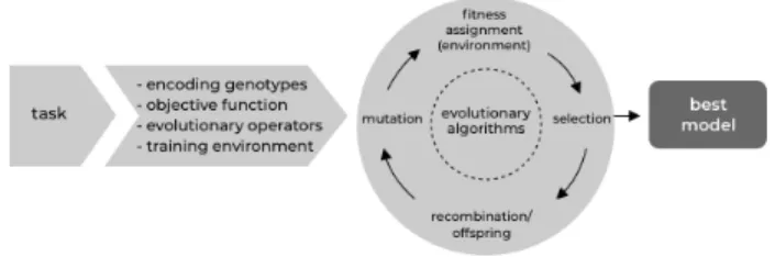
EAs [21] [22] are a class of population-based, stochastic search techniques inspired by biological evolution. These types of algorithms share the same types of evolution mechanics as genetics: mutation, fitness assignment, selection and offspring. The evolutionary mechanics and configuration vary from one algorithm to another. However, they can be summarized as a population of agents P(θ), which represents a potential solution to an optimization problem. The performance of each agent θi is evaluated over each generation through a fitness
function F(θi). Then some agents are selected to become
parents and generate the next offspring, the offspring are mutated by defined evolutionary techniques. Evolution takes
Fig. 1. Evolutionary algorithm cycle. Adapted from geneticprogramming.com.
place by repeating this process through N cycles, or until a stopping criterion is met (Back, 1996).
Following the application of EAs to DNNs the approach called neuroevolution emerged, which evolves a DNN until the network agent best suited for a defined task is found, as shown in Fig. 1. These approaches move from classical learning methods to evolutionary methods, where DNN characteristics such as architecture, weights, and in some cases, hyperparam-eters are encoded into genomes. The genomes are then evolved using an EA according to a performance criterion. According to Stanleyet al.[23], the use of EAs to design ANNs presents the advantages of high parallelization and diversity in the search space of solutions. Another advantage of using EAs is that if one is combined with a notion of quality (e.g., to maximize reward) during exploration, the population will disseminate looking for different strategies and will quickly point to the global optimum.
In addition to evolution strategies, another algorithm used to optimize DNNs is called a covariance matrix adaptation evolution strategy (CMA-ES) [13]. CMA-ES is a type of black-box optimization technique based on EA for non-linear and non-convex problems. CMA-ES is considered state-of-the-art in evolutionary computation and has been adopted as one of the standard tools for continuous optimization problems. This approach creates a covariance matrix describing the cor-relations between decision variables. Then, through evolution mechanics, the matrix likelihood is maximized generating successful solutions. The CMA-ES state variables, for a space of dimensionN, are given by the distribution meanm∈Rn,
the step size σ > 0 and the covariance matrix C ∈ Rnxn.
CMA-ES is an iterative algorithm that, in each of its iterations, samples λ candidate solutions from a multivariate normal distribution, evaluates them and then adjusts the sampling distribution used for the next iteration [24].
III. RELATEDWORK
Electricity consumption can be represented through time series models. Every electricity consumption dataset presents unique properties related to the location, weather, and social factors where it was collected. Hence, because of this vari-ability, each dataset is challenging to analyze and model. An important branch of statistical machine learning that can learn patterns from data is DNN models. DNN together with high computing power has shown excellent performance for various prediction tasks. Zheng et al.[10] presented a method using LSTM for load forecasting on smart grids for a city. Marinoet
al. [25], presented their approach to forecast building energy consumption using DNN. Specifically, for residential load forecasting, Zhang et al.[26] presented the perspective for a single house load forecasting using SVR modelling. Recently, Wang et al.[27] presented an approach using a probabilistic method applied to LSTM. Most of the improvements presented are related to enhancing load forecasting by improving the ANN and finding out how to learn the weights of the neurons effectively. Nevertheless, we have not found work that has been developed to improve the architecture of a DNN for time series forecasting. Furthermore, as far as the authors know, no work has been done to automate architecture search for load forecasting.
In STLF, EAs have been commonly used to optimize hyperparameters in forecasting models such as the work pre-sented by Zhang et al. [28] to tune SVR-based models with differential evolution. In one of the most recent studies using EA, Zenget al.[10] combined particle optimization techniques with a method called an extreme learning machine. In another study, Bouktifet al.[29] proposed to use LSTM models using feature selection combined with a genetic algorithm for load forecasting. In terms of neuroevolution techniques applied to load forecasting, Srinivasan [30] presented an approach to evolve an ANN. In this approach, the architecture was fixed at three layers, and only the hyperparameters and weights of the ANN were evolved.
In contrast, the techniques presented so far have been focussed on tuning model hyperparameters, or in the best scenario, to evolve the DNN weights. Few approaches have focussed on searching for the best DNN architecture otherwise than by image optimization. The approach called weight ag-nostic neural network presented by Gaier and Ha [31] focussed on evolving a robust architecture for reinforcement learning tasks, which can be used as a research base for additional tasks such as time series forecasting.
This paper proposes a method to find a deep neural network centred on architecture evolution (DNN-CAE) for short-term load forecasting. The method focusses on NAS using EA techniques. DNN-CAE search is used to find the optimal architecture leaving aside the importance of the weights while the model is trained. Finally, after the best architecture has been found, the weights are tuned using a CMA-ES algorithm, improving load forecasting performance.
IV. DNN-CAE METHODOLOGY
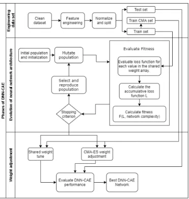
The approach presented in this paper has been implemented in three phases, as shown in Fig. 2, which are: engineering the dataset, evolution of the neural network architecture and weight adjustment. Each one of these phases is explained in detail next:
A. Phase 1: engineering the dataset
In this phase, three steps are performed before the dataset is split between training and test sets. The steps of cleaning the dataset, feature engineering and normalizing and splitting the
Fig. 2. Framework for the DNN-CAE model.
dataset are essential for adequate training and performance of the algorithm.
1) Cleaning the dataset: The dataset is cleaned by remov-ing all NaN and duplicated values. In addition, anomalies are detected and removed, such as non-sequential data, values with wrong units and filling missing values. After this step, the whole data collected become consistent.
2) Feature engineering: In this step, the number of features in the dataset is increased. Weather attributes related to the same date and time as the data are added, such as temperature and weather conditions as categorical values. New features are also added to the dataset, such as day of the week, is weekday, is weekend, is holiday, and the season of the year. Finally, some cyclic features such as month, day, hour and weekday are transformed through sine and cosine functions into cyclic values. Past values from the same set as new features are also added, such as previous target values from the last hour up to the last 48 hours. Averages for the previous 24 and 48 hours, and values for the last week at the same time, for the last month, and for last year.
3) Normalizing and splitting the dataset: In this step, the whole dataset is normalized by applying min-max normaliza-tion as given in (1). Then, the dataset is split into training and test sets with a proportion of 80%-20%. During evolution of the DNN, the model is trained with the training set. Then the CMA-ES algorithm uses the last 20% of the training set to adjust the weights. This approach is taken to evolve the DNN’s weights with similar behavior as the test set, but with the training set data. Carrying out this procedure also improves model accuracy for the weight adjustment phase. Finally, the test set is used for model performance measurement.
TABLE I
DESCRIPTION OF PARAMETERS USED DURING EVOLUTION. Parameter Description
Ps Population size of network agents.
Swb Shared weights negative and positive boundaries.
Sws Shared weights list size.
Gmax Maximum number of generations.
Fb Fitness threshold.
Mnode Probability of inserting a node.
Mconn Probability of adding a connection.
Mact Probability of changing an activation function.
Afl List of available activation functions.
Ts Tournament size.
x= xi−xmin
xmax−xmin
(1)
B. Phase 2: evolution of the neural network architecture
In this phase, NAS with an EA optimization method is per-formed. This approach focusses on the architecture evolution by reducing the importance of the weights. In general terms, during the evolution phase, the architecture search avoids weight training and adjustment by sampling on different fitness measurements using shared weights values. Each network agent is evaluated over a set of shared weights values, and the cumulative loss function is recorded. Finally, the parents that will create the offspring are chosen by tournament selection. This process is repeated following evolution mechanics until the model with the best unadjusted-weights-architecture is found. Table I describes the various parameters used during search architecture evolution.
Algorithm 1 describes the evolution of the neural network architecture for the DNN-CAE approach, which is illustrated in Fig. 2. In the following subsections, each component of the neural network architecture evolution as shown in Fig. 2 will be described; the descriptions refer to the corresponding lines in Algorithm 1.
1) Initial population and initialization: An initial popu-lation with a minimal neural network topology is created. Each network agent θi starts with an input layer and one
output layer. In this step, no connections are made between the input and output layers. The size of the network agent populationP(θ)is set according toPs. In addition, during this
step, the various values for the shared weights wj ∈asw are
defined with (2). The array of shared weightsasw, the current
generationg and the best fitness for the current generationfg
are also initialized. This step is performed only once during the evolution process as shown in line 3 of Algorithm 1.
wj =Swb −1 + 2j Sws ,∀j= 0,1, . . . , Sws (2) 2) Stopping criterion: Here the algorithm checks whether
GmaxorFbhas been reached. If one of these criteria has been
reached, the evolution interaction stops, the best agentθbestis
saved, and the procedure moves forward to the next phase. If neither of the criteria is satisfied, the iterative evolution process continues. Both parameters Gmax andFb are set in line 1 of
Algorithm 1: Architecture evolution
1 Parameters:Ps,Swb,Sws,Gmax,b,Mconn,Mnode,Afl,Ts.
2 Output:θbestwith best fitness.
3 Initialize:P(θ)of sizePs,asw with (2),g= 0,fg=−∞.
4 while g < Gmax∧fg< Fbdo
/* Mutate population */
5 fori= 1, . . . , Psθi∈P(θi)do
- insert a node with probabilityMnode,
- add a connection with probabilityMconn,
- change an existing activation function to another listed inAfl. 6 end /* Evaluate fitness */ 7 fori= 1, . . . , Psθi∈P(θi)do 8 forj= 0,1, . . . , Swswj∈asw do 9 Calculatelj(θi, wj)with (3). 10 end 11 CalculateL(θi) =Plj(θi, wj). 12 CalculateF(θi)with (4). 13 end
/* Select and reproduce */
14 Initialize:offspring. 15 fori= 1, . . . , Psdo
16 Randomly selectTscandidates fromP(θi).
17 Pick upθiwith the best fitness from the tournament and
copy it to the offspring. 18 end 19 P(θi)←−offspring. 20 fg←−bestF(θi)∈P(θi). 21 g=g+ 1. 22 end 23 θbest←−θ(fg)
Algorithm 1, the while-loop in line 4 runs until one or both criteria are satisfied.
3) Mutate population: To avoid local optima, mutation must be implemented over each agentθiin each new
genera-tion. Following the work of Gaier and Ha [31], each agentθi
enhances its performance by directly implementing one of the three possible mutations, which are 1) insert a node, 2) add a connection, and 3) change the activation function. The first two mutations were chosen because they enhance the behaviour and performance ofθi. Note that these mutations increase the
complexity of the architecture.
To insert a node, an existing connection between two nodes is split into two connections, and then a new node is added with a random activation function. To add a connection, two unconnected nodes not belonging to the same layer are ran-domly selected, and then a new connection is created. Finally, mutation of the activation function changes one function for another one that is randomly selected.
The first for-loop (lines 5 to 6) of Algorithm 1 performs the mutation step, with probabilities of inserting a node, adding a connection, and changing the activation function set by the parametersMnode,Mconn andMact, respectively. The list of
the allowed activation functions is given inAfl.
4) Evaluate fitness: This step is divided into three actions, as shown in Fig. 2, and lines (7 to 13) of Algorithm 1, which are 1) evaluate the loss function, 2) calculate cumulative loss function, and 3) calculate the fitness value for eachθi.
shared valuewj. Then the network agent’s performance over a
training set batch is evaluated, and the loss functionlj(θi, wj)
is calculated with (3), (lines 8 to 10) of Algorithm 1.
lj(θi, wj) =− batch
X
k=0
abs(ˆyk(θi, wj)−yk) (3)
where θi is the network agent to be evaluated, wj is the
shared weights value, yˆk(θi, wj) is the prediction for the
network evaluated with wj, and yk is the target values from
the training set. The loss function is negative because the algorithm minimizes the loss function over each generation.
The second action calculates the cumulative loss function
L(θi)(line 11). Here, the loss functionlj calculated for each wj are added together. Finally, the third action calculates each
network agent’s fitness F(θi) (line 12) of Algorithm 1. The
fitness function is stated in (4):
F(θi) =−L(θi)−Nc(θi)−Nn(θi) (4)
whereL(θi)is the cumulative loss function as calculated,Nc
is the total number of active connections in the network, and
Nn is the number of nodes in the network. The advantage of
using (4) is that when two agents present the same cumulative loss function; the agent with the simpler architecture receives the higher fitness score.
5) Select and reproduce: Among the possible parent se-lection techniques, tournament sese-lection was chosen because this method has given good results in NAS approaches such as those presented by Real et al. [17] and Liu et al. [15]. This characteristic avoids stagnation of the evolution process through dominance by the best-fitness individual and allows diversity during parent selection to create the next offspring. By using tournament selection (lines 14 to 18) of Algorithm 1, individuals are randomly selected according to the tournament size Ts. The best individuals from tournament selection are
part of the next generation of offspring. This process is repeated until Psis reached.
C. Phase 3: Weight adjustment
This phase receives the model with the best unadjusted-weights-architecture from phase 2 and, through weight adjust-ment, enhances DNN model performance. Consequently, in this phase, the weights are analyzed to create the DNN-CAE.
1) Shared weights tuning: In this step, the effect of the shared weights over the best unadjusted-weights-architecture model is analyzed. The model is tested over the range of values specified by the parameters Swb. By reducing the sampling
step size, the shared weights value that maximizes the model accuracy is found. Then this shared value, which minimizes the error, is picked up and sent to the DNN-CAE performance evaluation step, as shown in Fig. 2.
2) CMA-ES weight adjustment: In this step, the CMA-ES technique is used to evolve the weights of the best unadjusted-weights-architecture model and tune the DNN. This step uses what can be considered a baseline version, featuring non-elitist (µ, λ) selection. All tuning constants are set to their default
values, as stipulated by Hansen [24]. In this step, the CMA-ES algorithm interacts with the model until it finds the best set of individual values for the weights and passes these values on to the next step.
3) DNN-CAE performance evaluation: Finally, in this step, the best unadjusted-weights-architecture model with both op-timized shared weights and CMA-ES weight values is tested. For this purpose, the model performance over the test set is evaluated, first with the values of the shared weights and then with the CMA-ES values. Finally, the set of weights that best enhances performance is selected. In consequence, the DNN-CAE model is the best architecture found by the architecture centred evolution approach and the best set of weights. Finally, the RMSE (5) and the MAPE (6) are calculated to measure the model performance over the test set.
RM SE= v u u t 1 n n X k=0 (ybk−yk) 2 (5) M AP E= 1 n n X k=0 b yk−yk yk x100 (6)
whereybkdenotes the predicted consumption,yk denotes the
actual electricity consumption of the household, andn is the number of observations.
V. EXPERIMENTS
DNN-CAE is used for short-term load forecasting as a DNN model that accesses the inputs from the current time step and previous electricity consumption values to forecast the next hour’s consumption. All the models and experiments were run on a Linux server with 24 Intel(R) Xeon(R) E5-2630 v2 processors.
A. Data
Patterns in residential electricity consumption present com-plex and non-linear relationships, which makes them a chal-lenging problem. The characteristics of electricity consump-tion depend on the weekday and the hour of the day, as shown in Fig. 3. Residential load consumption data for one household were provided by the London Hydro utility company. The raw dataset from smart meters contains electricity consumption data measured in kilowatt-hours (kW-h) on a one-hour time scale. Historical hourly weather and temperature data were obtained from the Canadian Government Official Website [32]. The dataset contains hourly data from January 1, 2014, to December 31, 2016.
B. Shared weights range evaluation and parameter selection
To run the model adequately, it is necessary to evaluate the range of operation for the various shared weights values. Table II shows the results for shared weights performance tests, each carried out with a different range of shared weights and different sampling steps size. In each performance test, the median fitness and the best individual fitness were measured.
TABLE II
SHARED WEIGHTS PERFORMANCE*TESTS. Shared weights values Best agent
fitness Best possible shared weight Range between Sampling step [-10, 10] 1.0 3000 0 0.5 6130 0 [-5, 5] 1.00.5 10201550 00 [-2, 2] 1.0 663 0.1 0.5 419 0.1 [-1.5, 1.5] 0.5 96 0.4 [-1, 1] 0.1 85 0.4
*Performance test withGmax= 256andPs= 128.
Then the best shared weights value was picked, and the DNN-CAE weights were adjusted to measure fitness performance.
Table II shows that the best fitness values increase as the range of evaluation becomes larger. Consequently, conver-gence to the best picked weight is lost. In contrast, if the selected range narrows, the best fitness value decreases and begins to converge to a value different than zero. Based on the results from Table II, the limits for Swb were set to [-1,
1] with Sws= 0.1.
C. Experiment 1: DNN-CAE for residential load forecasting
The parameters selected to run Experiment 1 are presented in Table III. These parameters were chosen empirically after several model runs. Fig. 4 shows the model evolution over 1024 generations. The time that took to evolve the model was 11 hours and 46 minutes, with a depth of 644 nodes.
1) DNN-CAE shared-weight fitness evaluation: Fig. 5 shows the results for shared-weight DNN-CAE fitness perfor-mance over the test set. During this evaluation, the model was tested within the range [-1, 1]. Fig. 5 shows that the DNN-CAE best performance for shared weights occurred between 0.6 and 0.8. The maximum fitness value was found at 0.71, with fitness of -45.44.
2) CMA-ES adjustment performance evaluation: After run-ning the CMA-ES algorithm to adjust the weights individually, the DNN-CAE model performance over the test set was
evalu-Fig. 3. Residential daily electricity consumption for a random week in 2015.
TABLE III
PARAMETERS USED DURING EXPERIMENT1
Parameter Value Ps 128 Gmax 1024 b 0.10 Mconn 0.25 Mnode 0.25 Maf 0.50
Afl tanh, sigmoid, inverse, absolute, ReLulinear, step, sine, gaussian,
Ts 32
Fig. 4. Fitness graph showing fitness evolution over each generation. The first 30 generations’ values were removed for better visualization.
ated. The CMA-ES weight evolution ran over 500 generations for 2 hours and 46 minutes.
3) DNN-CAE tuned performance: After tuning the DNN-CAE model with the best values for each adjustment tech-nique, the evaluation is conducted. Three experiments were performed for each: best fitness, RMSE, and MAPE; the average of the values was calculated and are presented in Table IV. For RMSE and MAPE, the lower the values, the more accurate the model is. Fig. 6 shows how the model fit the test set over the first week of the test set for both techniques.
D. Experiment 2: Evolution behaviour based on activation function selection
In this experiment, three models were evolved to analyze their evolution behaviour with restriction on the available
Fig. 5. DNN-CAE fitness performance for shared-weight within the range [-1, 1] andSws= 0.01.
TABLE IV
EXPERIMENT1PERFORMANCE TUNING TECHNIQUES COMPARISON
Tuning technique Best fitness RMSE (kW-h) MAPE (%) Shared weights -61.41 0.2623 22.18
TABLE V
PARAMETERS MODIFIED DURING EXPERIMENT2 Parameter WALF-3AF WALF-5AF WALD-9AF
Afl inverse, abs, ReLu
tanh, sigmoid, inverse, abs, ReLu
linear, step, sine, gaussian, tanh, sigmoid, inverse,
abs, ReLu
Gmax 500
TABLE VI
COMPARATIVE RESULTS FROM RESTRICTING ACTIVATION FUNCTIONS
Model Evolution time (minutes) CMA time (minutes) MAPE (%) Shared weights CMA-ES WALF-3AF 178 35 18.80 8.16 WALF-5AF 93 57 28.37 7.74 WALF-9AF 122 71 31.32 9.49
activation functions. The first model, CAE-3AF, had only inverse, absolute and ReLu activation functions set; the second model, CAE-5AF, had the most used activation functions available, which were: sigmoid, hyperbolic tangent, inverse, absolute and ReLu. Finally, the third model, CAE-9AF, had all the activation functions available. The three models were evolved with the same parameters as in Experiment 1, with modifications only toPs andAfl. Table V shows the
param-eters values as modified to run Experiment 2.
For this experiment, the error threshold was removed and the models evolved until the maximum number of generations was reached. The time required to evolve each model was also recorded. Table VI presents the results of this experiment.
Clearly, CAE-9AF presents a higher error than the other two models, which could have been a consequence of extensive search among all the activation functions. On the other hand, CAE-3AF and CAE-5AF showed closest error values after 500 generations. Nevertheless, the model with five activation functions was 29% faster than the model with three activation functions. So far, these experiments have determined that the CAE-5AF model performs well and that the time to evolve it is optimal.
Fig. 6. DNN-CAE performance for shared weights and CMA-ES adjustment. For visualization purposes, only 48 hours from the first week of the test set is shown.
TABLE VII
BENCHMARK MODEL PARAMETERS
Method # Features # Hidden layers # Hidden nodes/layer Vanilla LSTM 1 2 5 MLP 33 2 20 LSTM features 6 2 12 LSTM one-shot 33 2 20 TABLE VIII
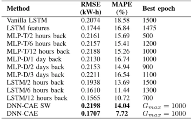
LOAD FORECASTING EVALUATION SUMMARY
Method (kW-h)RMSE MAPE(%) Best epoch Vanilla LSTM 0.2074 18.58 1500 LSTM features 0.1744 16.84 1475 MLP-T/2 hours back 0.2161 15.69 500 MLP-T/6 hours back 0.2157 15.41 1200 MLP-T/12 hours back 0.2188 15.26 1000 MLP-D/1 day back 0.2130 16.74 1000 MLP-D/2 days back 0.2153 14.94 900 MLP-D/3 days back 0.2211 16.54 1100 LSTM/2 hours back 0.1938 13.69 1500 LSTM/6 hours back 0.1610 11.44 1300 LSTM/12 hours back 0.1565 10.72 700 DNN-CAE SW 0.2198 14.04 Gmax= 1000 DNN-CAE 0.1707 7.72 Gmax= 1000
E. Experiment 3: Benchmark comparison
In Experiment 3, a benchmark comparison was performed between the proposed DNN-CAE and conventional ANN methods. For purpose of this comparison, the benchmark presented by Konget al. [33] was reproduced. The methods selected for the comparison were MLP, vanilla LSTM and LSTM One-shot (LSTMOS). Vanilla LSTM is the simplest method with only one input for the residential load time series. However, LSTM-features model has additional features for training, such as time, weekdays and holidays. LSTMOS [33] is state-of-the-art in residential load forecasting. Table VII presents the parameters used to configure the ANN as presented in [33].
MLP and LSTMOS were trained with different backward time steps. To follow the convention used in [33] -T is for backward hour steps, and -D is for backward day steps. As Ta-ble VIII shows, the results of DNN-CAE with shared weights are close to those of the MLP method. After adjustment of the DNN-CAE weights the model accuracy surpassed the best LSTM one shot model by 3.0%. Therefore, DNN-CAE is a serious competitor among the listed algorithms for STLF task of residential load forecasting.
VI. CONCLUSIONS
This paper proposed an approach for NAS based on EAs, focusing on the architecture first during the evolution phase, which resulted in the creation of a neural architecture for short-term residential electrical load forecasting. Later, the model was tuned by adjusting the weights, which enhanced model performance. The evolution starts with simple neural architectures and grows in complexity as the model evolves. As shown, DNN-CAE has been optimized to work with a
single shared weights parameter over a range of shared weights values. Therefore, the model is easy to tune to achieve ac-ceptable performance with shared weights. Furthermore, using the CMA-ES technique the weights are adjusted individually, enhancing model accuracy. In addition, after running three different experiments, DNN-CAE showed accuracy in the range of 90%. The model presented in this work can be used in a general sense in other similar time series forecasting domains such as energy utility, weather, and finances.
DNN-CAE shared weights presented results similar to those from MLP. Furthermore, DNN-CAE after weights adjustment outperformed the LSTM one-shot method, which is the-state-of-the-art for residential load forecasting. The results presented in this work are the first of their kind applied to short-term load forecasting. As future work, the authors plan to investigate how to improve model accuracy. This paper has also evaluated model performance for only one residential dataset. In future work, DNN-CAE will be applied to create a general architecture for different homes in the same area, and then, by tuning the weights, the model will be able to adapt its forecast from one house to another. Finally, a sensitivity analysis will be performed on DNN-CAE to identify the importance each parameter plays on the model.
REFERENCES
[1] “International Energy Agency, world electricity per capita,” https://www.iea.org, accessed: 2020-03-30.
[2] W. Kong, Z. Y. Dong, D. J. Hill, F. Luo, and Y. Xu, “Short-Term Residential Load Forecasting Based on Resident Behaviour Learning,”
IEEE Transactions on Power Systems, vol. 33, no. 1, pp. 1087–1088, 1 2018.
[3] M. Imani and H. Ghassemian, “Residential load forecasting using wavelet and collaborative representation transforms,”Applied Energy, vol. 253, p. 113505, 11 2019.
[4] D. Alberg and M. Last, “Short-term load forecasting in smart meters with sliding window-based ARIMA algorithms,” Vietnam Journal of Computer Science, vol. 5, no. 3-4, pp. 241–249, 9 2018.
[5] Y. Chen, P. Xu, Y. Chu, W. Li, Y. Wu, L. Ni, Y. Bao, and K. Wang, “Short-term electrical load forecasting using the Support Vector Regres-sion (SVR) model to calculate the demand response baseline for office buildings,”Applied Energy, vol. 195, pp. 659–670, 6 2017.
[6] M. Q. Raza and A. Khosravi, “A review on artificial intelligence based load demand forecasting techniques for smart grid and buildings,”
Renewable and Sustainable Energy Reviews, vol. 50, pp. 1352–1372, 10 2015.
[7] Y. T. Chae, R. Horesh, Y. Hwang, and Y. M. Lee, “Artificial neural net-work model for forecasting sub-hourly electricity usage in commercial buildings,”Energy and Buildings, vol. 111, pp. 184–194, 1 2016. [8] A. Ghani, M. Baqar, I. E. Khuda, K. Raza, and S. Yasin, “Artificial
Neural Network Based Electrical Load Prediction of Karachi City - A Cross-sectional Study,” in 2019 13th International Conference on Mathematics, Actuarial Science, Computer Science and Statistics (MACS). IEEE, 12 2019, pp. 1–5.
[9] S. Fallah, R. Deo, M. Shojafar, M. Conti, and S. Shamshirband, “Computational Intelligence Approaches for Energy Load Forecasting in Smart Energy Management Grids: State of the Art, Future Challenges, and Research Directions,”Energies, vol. 11, no. 3, p. 596, 3 2018. [10] Jian Zheng, Cencen Xu, Ziang Zhang, and Xiaohua Li, “Electric load
forecasting in smart grids using Long-Short-Term-Memory based Recur-rent Neural Network,” in2017 51st Annual Conference on Information Sciences and Systems (CISS). IEEE, 3 2017, pp. 1–6.
[11] B. Zhang, J. L. Wu, and P. C. Chang, “A multiple time series-based recurrent neural network for short-term load forecasting,”Soft Computing, vol. 22, no. 12, pp. 4099–4112, 6 2018.
[12] T. Elsken, J. H. Metzen, and F. Hutter, “Neural architecture search: A survey,”arXiv preprint arXiv:1808.05377, 2018.
[13] N. Hansen and A. Ostermeier, “Completely Derandomized Self-Adaptation in Evolution Strategies,”Evolutionary Computation, vol. 9, no. 2, pp. 159–195, 6 2001.
[14] B. Zoph, V. Vasudevan, J. Shlens, and Q. V. Le, “Learning Transferable Architectures for Scalable Image Recognition,”CVPR, pp. 8697–8710, 2018.
[15] C. Liu, B. Zoph, M. Neumann, J. Shlens, W. Hua, L.-J. Li, L. Fei-Fei, A. Yuille, J. Huang, and K. Murphy, “Progressive Neural Architecture Search,” inLecture Notes in Computer Science (including subseries Lec-ture Notes in Artificial Intelligence and LecLec-ture Notes in Bioinformatics), 2018, vol. 11205 LNCS, pp. 19–35.
[16] Z. Zhong, Z. Yang, B. Deng, J. Yan, W. Wu, J. Shao, and C.-L. Liu, “BlockQNN: Efficient Block-wise Neural Network Architecture Genera-tion,”IEEE Transactions on Pattern Analysis and Machine Intelligence, pp. 1–1, 8 2020.
[17] E. Real, S. Moore, A. Selle, S. Saxena, Y. L. Suematsu, J. Tan, Q. V. Le, and A. Kurakin, “Large-scale evolution of image classifiers,” in
34th International Conference on Machine Learning, ICML 2017, vol. 6, 2017, pp. 4429–4446.
[18] T. Wei, C. Wang, Y. Rui, and C. W. Chen, “Network morphism,” in
33rd International Conference on Machine Learning, ICML 2016, vol. 2, 2016, pp. 842–850.
[19] R. Luo, F. Tian, T. Qin, E. Chen, and T. Y. Liu, “Neural architecture optimization,” inAdvances in Neural Information Processing Systems, vol. 2018-Decem, 2018, pp. 7816–7827.
[20] A. Brock, T. Lim, J. M. Ritchie, and N. Weston, “SmaSH: One-shot model architecture search through hypernetworks,” in6th International Conference on Learning Representations, ICLR 2018 - Conference Track Proceedings, 8 2018.
[21] J. Holland, “Adaptation in artificial and natural systems,”Ann Arbor: The University of Michigan Press, p. 232, 1975.
[22] I. Rechenberg, “Evolutionsstrategien,” in Simulationsmethoden in der Medizin und Biologie. Springer, 1978, pp. 83–114.
[23] K. O. Stanley, J. Clune, J. Lehman, and R. Miikkulainen, “Designing neural networks through neuroevolution,”Nature Machine Intelligence, vol. 1, no. 1, pp. 24–35, 1 2019.
[24] N. Hansen, “The cma evolution strategy: A tutorial,” arXiv preprint arXiv:1604.00772, 2016.
[25] D. L. Marino, K. Amarasinghe, and M. Manic, “Building energy load forecasting using Deep Neural Networks,” in IECON 2016 - 42nd Annual Conference of the IEEE Industrial Electronics Society. IEEE, 10 2016, pp. 7046–7051.
[26] X. M. Zhang, K. Grolinger, M. A. Capretz, and L. Seewald, “Forecast-ing residential energy consumption: S“Forecast-ingle household perspective,” in
2018 17th IEEE International Conference on Machine Learning and Applications (ICMLA). IEEE, 2018, pp. 110–117.
[27] Y. Wang, D. Gan, M. Sun, N. Zhang, Z. Lu, and C. Kang, “Probabilistic individual load forecasting using pinball loss guided LSTM,”Applied Energy, vol. 235, pp. 10–20, 2 2019.
[28] F. Zhang, C. Deb, S. E. Lee, J. Yang, and K. W. Shah, “Time series forecasting for building energy consumption using weighted support vector regression with differential evolution optimization technique,”
Energy and Buildings, vol. 126, pp. 94–103, 2016.
[29] S. Bouktif, A. Fiaz, A. Ouni, and M. Serhani, “Optimal Deep Learning LSTM Model for Electric Load Forecasting using Feature Selection and Genetic Algorithm: Comparison with Machine Learning Approaches †,”
Energies, vol. 11, no. 7, p. 1636, 6 2018.
[30] D. Srinivasan, “Evolving artificial neural networks for short term load forecasting,”Neurocomputing, vol. 23, no. 1-3, pp. 265–276, 12 1998. [31] A. Gaier and D. Ha, “Weight agnostic neural networks,” inAdvances in
Neural Information Processing Systems, 2019, pp. 5364–5378. [32] “Government of Canada, historical climate data,”
https://climate.weather.gc.ca, accessed: 2020-03-28.
[33] W. Kong, Z. Y. Dong, Y. Jia, D. J. Hill, Y. Xu, and Y. Zhang, “Short-term residential load forecasting based on lstm recurrent neural network,”