Worcester Polytechnic Institute
DigitalCommons@WPI
Computer Science Faculty Publications
Department of Computer Science
9-29-2012
A Practical Regularity Partitioning Algorithm and
its Applications in Clustering
Gábor N. Sárközy
Worcester Polytechnic Institute, [email protected]
Fei Song
Worcester Polytechnic Institute, [email protected]
Endre Szemerédi
Rutgers University - New Brunswick/Piscataway, [email protected]
Follow this and additional works at:
http://digitalcommons.wpi.edu/computerscience-pubs
Part of the
Computer Sciences Commons
This Other is brought to you for free and open access by the Department of Computer Science at DigitalCommons@WPI. It has been accepted for inclusion in Computer Science Faculty Publications by an authorized administrator of DigitalCommons@WPI.
Suggested Citation
Sárközy, Gábor N. , Song, Fei , Szemerédi, Endre (2012). A Practical Regularity Partitioning Algorithm and its Applications in Clustering. .
WPI-CS-TR-12-05 September 2012
A Practical Regularity Partitioning Algorithm and its
Applications in Clustering
by
G´
abor N. S´
ark¨
ozy
Fei Song
Endre Szemer´
edi
Shubhendu Trivedi
Computer Science
Technical Report
Series
WORCESTER POLYTECHNIC INSTITUTE
Computer Science Department
A Practical Regularity Partitioning Algorithm and its
Applications in Clustering
G´
abor N. S´
ark¨
ozy
∗†
, Fei Song
†
, Endre Szemer´
edi
‡
, Shubhendu Trivedi
†
†
Computer Science Department
Worcester Polytechnic Institute
Worcester, MA 01609
‡
Computer Science Department
Rutgers University
New Brunswick, NJ 08901
September 29, 2012
Abstract
In this paper we introduce a new clustering technique calledRegularity Clustering. This new technique is based on the practical variants of the two constructive versions of the Regularity Lemma, a very useful tool in graph theory. The lemma claims that every graph can be parti-tioned into pseudo-random graphs. While the Regularity Lemma has become very important in proving theoretical results, it has no direct practical applications so far. An important reason for this lack of practical applications is that the graph under consideration has to be astronomi-cally large. This requirement makes its application restrictive in practice where graphs typiastronomi-cally are much smaller. In this paper we propose modifications of the constructive versions of the Regularity Lemma that work for smaller graphs as well. We call this the Practical Regularity partitioning algorithm. The partition obtained by this is used to build the reduced graph which can be viewed as a compressed representation of the original graph. Then we apply a pairwise clustering method such as spectral clustering on this reduced graph to get a clustering of the original graph that we call Regularity Clustering. We present results of using Regularity Cluster-ing on a number of benchmark datasets and compare them with standard clusterCluster-ing techniques, such ask-means and spectral clustering. These empirical results are very encouraging. Thus in this paper we report an attempt to harness the power of the Regularity Lemma for real-world applications.
1
Introduction
The Regularity lemma of Szemer´edi [20] has proved to be a very useful tool in graph theory. It was initially developed as an auxiliary lemma to prove a long standing conjecture of Erd˝os and Tur´an[4] on arithmetic progressions, which stated that sequences of integers with positive upper
density must contain arbitrarily long arithmetic progressions. Now the Regularity Lemma by itself has become an important tool and found numerous other applications (see [14]). Based on the Regularity Lemma and the Blow-up Lemma [13] the Regularity method has been developed that has been quite successful in a number of applications in graph theory (e.g. [11]). However, one major disadvantage of these applications and the Regularity Lemma is that they are mainly theoretical, they work only for astronomically large graphs as the Regularity Lemma can be applied only for such large graphs. Indeed, to find theε-regular partition in the Regularity Lemma, the number of vertices must be a tower of 2’s with height proportional toε−5. Furthermore, Gowers demonstrated
[8] that a tower bound is necessary.
The basic content of the Regularity Lemma could be described by saying that every graph can, in some sense, be partitioned into random graphs. Since random graphs of a given edge density are much easier to treat than all graphs of the same edge-density, the Regularity Lemma helps us to carry over results that are trivial for random graphs to the class of all graphs with a given number of edges. We are especially interested in harnessing the power of the Regularity Lemma for clustering data. Graph partitioning methods for clustering and segmentation have become quite popular in the past decade because of representative ease of data with graphs and the strong theoretical underpinnings that accompany the same.
In this paper we propose a general methodology to make the Regularity Lemma more useful in practice. To make it truly applicable, instead of constructing a provably regular partition we construct an approximately regular partition. This partition behaves just like a regular partition (especially for graphs appearing in practice) and yet it does not require the large number of vertices as mandated by the original Regularity Lemma. Then this approximately regular partition is used for performing clustering. We call the resulting new clustering techniqueRegularity clustering. We present comparisons with standard clustering methods such ask-means and spectral clustering and the results are very encouraging.
To present our attempt and the results obtained, the paper is organized as follows: In section 2 we discuss briefly some prior attempts to apply the Regularity Lemma in practical settings and place our work in contrast to those. In Section 3 we discuss clustering in general and also present a popular spectral clustering algorithm that is used later on the reduced graph. We also point out what are the possible ways to improve its running time. In Section 4 we give some definitions and general notation. In Section 5 we present two constructive versions of the Regularity Lemma (the original lemma was non-constructive). Furthermore, in this section we point out the various problems arising when we attempt to apply the lemma in real-world applications. In Section 6 we discuss how the constructive Regularity Lemmas could be modified to make them truly applicable for real-world problems where the graphs typically are much smaller, say have a few thousand vertices only. In Section 7 we show how this Practical Regularity partitioning algorithm can be applied to develop a new clustering technique. In Section 8, we present an extensive empirical validation of our method. Section 9 is spent in discussing the various possible future directions of work.
2
Prior Applications of the Regularity Lemma
As we discussed above so far the Regularity Lemma has been “well beyond the realms of any practical applications” [10], the existing applications have been theoretical,mathematical. The only practical application attempt of the Regularity Lemma to the best of our knowledge is by Sperotto and Pelillo [19], where they use the Regularity Lemma as a pre-processing step. They give some interesting ideas on how the Regularity Lemma might be used, however they do not give too many details. Taking leads from some of their ideas we give a much more thorough analysis of the modifications
needed in order to make the lemma applicable in practice. Furthermore, they only give results for using the constructive version by Alon et al[1], here we implement the version proposed by Frieze and Kannan [6] as well. We also give a far more extensive empirical validation; we use 12 datasets instead of 3.
3
Clustering
Out of the various modern clustering techniques, spectral clustering has become one of the most popular. This has happened due to not only its superior performance over the traditional clustering techniques, but also due to the strong theoretical underpinnings in spectral graph theory and its ease of implementation. It has many advantages over the more traditional clustering methods such as k-means and expectation maximization (EM). The most important is its ability to handle datasets that have arbitrary shaped clusters. Methods such as k-means and EM are based on estimating explicit models of the data. Such methods fail spectacularly when the data is organized in very irregular and complex clusters. Spectral clustering on the other hand does not work by estimating explicit models of the data but does so by analysing the spectrum of the Graph Laplacian. This is useful as the top few eigenvectors can unfold the data manifold to form meaningful clusters.
In this work we employ spectral clustering on the reduced graph (which is an essence of the original graph), even though any other pairwise clustering method could be used. The algorithm that we employ is due to Ng, Jordan and Weiss [16]. Despite various advantages of spectral clustering, one major problem is that for large datasets it is very computationally intensive. And understandably this has received a lot of attention recently. As originally stated, the spectral clustering pipeline has two main bottlenecks: First, computing the affinity matrix of the pairwise distances between datapoints, and second, once we have the affinity matrix the finding of the eigendecomposition. Many ways have been suggested to solve these problems more efficiently. One approach is not to use an all-connected graph but a k-nearest neighbour graph in which each data point is typically connected to lognneighboring datapoints(wherenis the number of data-points). This considerably speeds up the process of finding the affinity matrix, however it has a drawback that by taking nearest neighbors we might miss something interesting in the global structure of the data. A method to remedy this is the Nystr¨om method which takes a random sample of the entire dataset (thus preserving the global structure in a sense) and then doing spectral clustering on this much smaller sample. The results are then extended to all other points in the data set [5].
Our work is quite different from such methods. The speed-up is primarily in the second stage where eigendecomposition is to be done. The original graph is represented by a reduced graph which is much smaller and hence eigendecomposition of this reduced graph can significantly ease the computational load. Further work on a practical variant of the sparse Regularity Lemma could be useful in a speed-up in the first stage, too.
4
Notation and Definitions
Below we introduce some notation and definitions for describing the Regularity Lemma and our methodology.
Let G= (V, E) denote a graph, whereV is the set of vertices andE is the set of edges. When A, B are disjoint subsets ofV, the number of edges with one endpoint in A and the other inB is denoted bye(A, B). WhenAandBare nonempty, we define thedensityof edges betweenAandB asd(A, B) =e|(AA,B||B|). The most important concept is the following.
Definition 1.The bipartite graph G= (A, B, E)isε-regularif for everyX ⊂A,Y ⊂B satisfying:
|X|> ε|A|, |Y|> ε|B|,we have |d(X, Y)−d(A, B)|< ε,otherwise it isε-irregular.
Roughly speaking this means that in anε-regular bipartite graph the edge density betweenanytwo relatively large subsets is about the same as the original edge density. In effect this implies that all the edges are distributed almost uniformly.
Definition 2. A partitionP of the vertex setV =V0∪V1∪. . .∪Vk of a graph G= (V, E)is called
an equitable partition if all the classes Vi,1 ≤i ≤k, have the same cardinality. V0 is called the
exceptional class.
Definition 3. For an equitable partition P of the vertex set V =V0∪V1∪. . .∪Vk of G= (V, E),
we associate a measure called theindex ofP (or the potential) which is defined by
ind(P) = 1 k2 k X s=1 k X t=s+1 d(Cs, Ct)2.
This will measure the progress towards anε-regular partition.
Definition 4. An equitable partition P of the vertex set V =V0∪V1∪. . .∪Vk of G= (V, E) is
calledε-regularif|V0|< ε|V|and all butεk2of the pairs (Vi, Vj)areε-regular where1≤i < j≤k.
With these definitions we are now in a position to state the Regularity Lemma.
5
The Regularity Lemma
Theorem 1 (Regularity Lemma [20]).For every positiveε >0and positive integertthere is an integer T =T(ε, t)such that every graph with n > T vertices has anε-regular partition intok+ 1
classes, where t≤k≤T.
In applications of the Regularity Lemma the concept of the reduced graphplays an important role.
Definition 5. Given an ε-regular partition of a graph G = (V, E) as provided by Theorem 1, we define the reduced graph GR as follows. The vertices of GR are associated to the classes in the
partition and the edges are associated to theε-regular pairs between classes with density above d.
The most important property of the reduced graph is that many properties ofGare inherited by GR. ThusGR can be treated as a representation of the original graphGalbeit with a much smaller
size, an “essence” of G. Then if we run any algorithm on GR instead of G we get a significant speed-up.
5.1
Algorithmic Versions of the Regularity Lemma
The original proof of the Regularity Lemma [20] does not give a method to construct a regular partition but only shows that one must exist. To apply the Regularity Lemma in practical settings, we need a constructive version. Alon et al. [1] were the first to give an algorithmic version. Since then a few other algorithmic versions have also been proposed [6], [12]. Below we present the details of the Alonet al. algorithm.
5.1.1 Alonet al. Version
Theorem 2 (Algorithmic Regularity Lemma [1]). For everyε >0 and every positive integer
tthere is an integerT =T(ε, t)such that every graph withn > T vertices has anε-regular partition intok+ 1classes, wheret≤k≤T. For every fixed ε >0 andt≥1 such a partition can be found in O(M(n)) sequential time, whereM(n) is the time for multiplying twon byn matrices with0,1
entries over the integers. The algorithm can be parallelized and implemented inN C1.
This result is somewhat surprising from a computational complexity point of view since as it was proved in [1] that the corresponding decision problem (checking whether a given partition is ε-regular) is co-NP-complete. Thus the search problem is easier than the decision problem. To describe this algorithm, we need a couple of lemmas.
Lemma 1 (Alon et al. [1]). Let H be a bipartite graph with equally sized classes|A|=|B|=n. Let 2n−1/4< ε < 161. There is an O(M(n))algorithm that verifies that H isε-regular or finds two subsetA0 ⊂A,B0 ⊂B,|A0| ≥ ε4
16n,|B
0| ≥ ε4
16n, such that|d(A, B)−d(A
0, B0)| ≥ε4. The algorithm
can be parallelized and implemented inN C1.
This lemma basically says that we can either verify that the pair is ε-regular or we provide certificates that it is not. The certificates are the subsets A0, B0 and they help to proceed to the next step in the algorithm. The next lemma describes the procedure to do the refinement from these certificates.
Lemma 2 (Szemer´edi [20]). Let G = (V, E) be a graph with n vertices. Let P be an equitable partition of the vertex set V = V0∪V1∪. . .∪Vk. Let γ >0 and let k be a positive integer such
that 4k >600γ−5. If more than γk2 pairs(Vs, Vt),1 ≤s < t≤k, areγ-irregular then there is an
equitable partitionQof V into1 +k4k classes, with the cardinality of the exceptional class being at most|V0|+4nk and such thatind(Q)> ind(P) +
γ5
20.
This lemma implies that whenever we have a partition that is notγ-regular, we can refine it into a new partition which has a better index (or potential) than the previous partition. The refinement procedure to do this is described below.
Refinement Algorithm: Given a γ-irregular equitable partition P of the vertex set V =V0∪
V1∪. . .∪Vk with γ=ε
4
16, construct a new partitionQ.
For each pair (Vs, Vt),1≤s < t≤k, we apply Lemma 1 with A=Vs,B =Vtand ε. If(Vs, Vt)is
found to be ε-regular we do nothing. Otherwise, the certificates partition Vs andVt into two parts
(namely the certificate and the complement). For a fixedswe do this for allt6=s. InVs, these sets
define the obvious equivalence relation with at most2k−1classes, namely two elements are equivalent
if they lie in the same partition part for every t6=s. The equivalence classes will be called atoms. Setm=b|Vi|
4kc,1≤i≤k. Then we construct our new partition Qby choosing a maximal collection
of pairwise disjoint subsets ofV such that every subset has cardinalitymand every atomAcontains exactly b|Am|c subsets; all other vertices are put in the exceptional class. The collection Q is an equitable partition ofV into at most 1 +k4k classes and the cardinality of its exceptional class is at
most|V0|+4nk.
Now we are ready to present the main algorithm.
Regular Partitioning Algorithm: Given a graph Gandε, construct aε-regular partition. 1. Initial partition: Arbitrarily divide the vertices of G into an equitable partition P1 with
2. Check regularity: For every pair(Vs, Vt)ofPi, verify if it isε-regular or findX ⊂Vs, Y ⊂ Vt,|X| ≥ ε 4 16|Vs|,|Y| ≥ ε 4 16|Vt|, such that |d(X, Y)−d(Vs, Vt)| ≥ε4.
3. Count regular pairs: If there are at most εk2i pairs that are not verified as ε-regular, then halt. Pi is anε-regular partition.
4. Refinement: Otherwise apply the Refinement Algorithm and Lemma 2, where P =Pi, k =
ki, γ= ε
4
16, and obtain a partitionQ with1 +ki4
ki classes.
5. Iteration: Let ki+1=ki4ki, Pi+1=Q, i=i+ 1, and go to step 2.
Since the index cannot exceed 1/2, the algorithm must halt after at mostd10γ−5eiterations (see
[1]). Unfortunately, in each iteration the number of classes increases to k4k from k. This implies
that the graphGmust be indeed astronomically large (a tower function) to ensure the completion of this procedure. As mentioned before, Gowers [8] proved that indeed this tower function is necessary in order to guarantee an ε-regular partition for all graphs. The size requirement of the algorithm above makes it impractical for real world situations where the number of vertices typically is a few thousand.
5.1.2 Frieze-Kannan Version
The Frieze-Kannan constructive version is quite similar to the above, the only difference is how to check regularity of the pairs in Step 2. Instead of Lemma 1, another lemma is used based on the computation of singular values of matrices. For the sake of completeness we present the details.
Lemma 3 (Frieze-Kannan [6]).LetW be anR×Cmatrix with|R|=pand|C|=qandW∞≤1
andγ be a positive real.
a If there exist S ⊆ R, T ⊆ C such that |S| ≥ γp,|T| ≥ γq and |W(S, T)| ≥ γ|S||T| then
σ1(W)≥γ3
√
pq (whereσ1 is the first singular value).
b Ifσ1(W)≥γ
√
pqthen there exist S⊆R, T ⊆C such that|S| ≥γ0p,|T| ≥γ0qandW(S, T)≥
γ0|S||T|, whereγ0 =108γ3. FurthermoremS, T can be constructed in polynomial time.
Combining Lemmas 2 and 3, we get an algorithm for finding anε-regular partition, quite similar to the Alonet al. version [1], which we present below:
Regular Partitioning Algorithm (Frieze-Kannan): Given a graph G and ε, construct a
ε-regular partition.
1. Initial partition: Arbitrarily divide the vertices of G into an equitable partition P1 with
classesV0, V1, . . . , Vb, where|V1|=bnbcand hence|V0|< b. Denote k1=b.
2. Check regularity: For every pair (Vs, Vt) of Pi, compute σ1(Wr,s). If the pair(Vr, Vs) are
not ε-regular then by Lemma 3 we obtain a proof that they are not notγ=ε9/108-regular.
3. Count regular pairs: If there are at most εk2
i pairs that produce proofs of nonγ-regularity,
then halt. Pi is anε-regular partition.
4. Refinement: Otherwise apply the Refinement Algorithm and Lemma 2, where P =Pi, k =
ki, γ= ε
9
108, and obtain a partitionP
0 with1 +k
i4ki classes.
5. Iteration: Let ki+1=ki4ki, Pi+1=P0, i=i+ 1, and go to step 2.
6
Modifications to the Constructive Version
We see that even the constructive versions are not directly applicable to real world scenarios. We note that the above algorithms have such restrictions because their aim is to be applicable to all
graphs. Thus, to make the regularity lemma truly applicable we would have to give up our goal that the lemma should work forevery graph and should be content with the fact that it works for
most graphs. To ensure that this happens, we modify the Regular Partitioning Algorithm(s) so that instead of constructing a regular partition, we find an approximately regular partition, which should be much easier to construct. We have the following 3 major modifications to the Regular Partitioning Algorithm.
Modification 1: We want to decrease the cardinality of atoms in each iteration. In the above Refinement Algorithm the cardinality of the atoms may be 2k−1, wherekis the number of classes
in the current partition. This is because the algorithm tries to find all the possibleε-irregular pairs such that this information can then be embedded into the subsequent refinement procedure. Hence potentially each class may be involved with up to (k−1) ε-irregular pairs. One way to avoid this problem is to bound this number. To do so, instead of using all theε-irregular pairs, we only use some of them. Specifically, in this paper, for each class we consider at most oneε-irregular pair that involves the given class. By doing this we reduce the number of atoms to at most 2. We observe that in spite of the crude approximation, this seems to work well in practice.
Modification 2: We want to bound the rate by which the class size decreases in each iteration. As we have at most 2 atoms for each class, we could significantly increasemused in the Refinement Algorithm asm = |Vi|
l , where a typical value ofl could be 3 or 4, much smaller than 4
k. We call
this user defined parameterl the refinement number.
Modification 3: Modification 2 might cause the size of the exceptional class to increase too fast. Indeed, by using a smallerl, we risk putting 1l portion of all vertices intoV0after each iteration.
To overcome this drawback, we “recycle” most ofV0, i.e. we move back most of the vertices from
V0. Here is the modified Refinement Algorithm.
Modified Refinement Algorithm: Given aγ-irregular equitable partitionP of the vertex set
V =V0∪V1∪. . .∪Vk with γ=ε
4
16 and refinement numberl, construct a new partition Q.
For each pair (Vs, Vt),1≤s < t≤k, we apply Lemma 1 withA=Vs,B=Vt andε. For a fixeds
if (Vs, Vt)is found to be ε-regular for all t6=s we do nothing, i.e. Vs is one atom. Otherwise, we
select oneε-irregular pair (Vs, Vt)randomly and the corresponding certificate partitionsVs into two
atoms. Setm=b|Vi|
l c,1≤i≤k. Then first we choose a maximal collectionQ
0 of pairwise disjoint
subsets of V such that every member of Q0 has cardinality m and every atom A contains exactly
b|mA|cmembers of Q0. Then we unite the leftover vertices in eachVs, if there are at leastmvertices
then we select one more subset of sizemfrom these vertices, we add these sets to Q0 and finally we
add all remaining vertices to the exceptional class, resulting in the partition Q. The collectionQis an equitable partition ofV into at most1 +lkclasses.
Now, we present our modified Regular Partitioning Algorithm. There are three main parameters to be selected by the user: ε, the refinement numberl and h, the minimum class size when we must halt the refinement procedure. The parameterhis used to ensure that if the class size has gone too small then the procedure should not continue.
Modified Regular Partitioning Algorithm (or the Practical Regularity Partitioning Algorithm): Given a graph Gand parametersε,l,h, construct an approx. ε-regular partition.
1. Initial partition: Arbitrarily divide the vertices of G into an equitable partition P1 with
classesV0, V1, . . . , Vl, where|V1|=bnlcand hence|V0|< l. Denote k1=l.
(Vs, Vt)of Pi, verify if it isε-regular or find X ⊂Vs, Y ⊂Vt,|X| ≥ ε 4 16|Vs|,|Y| ≥ ε4 16|Vt|, such that |d(X, Y)−d(Vs, Vt)| ≥ε4.
3. Count regular pairs: If there are at most εk2
i pairs that are not verified as ε-regular, then
halt. Pi is anε-regular partition.
4. Refinement: Otherwise apply the Modified Refinement Algorithm, whereP =Pi, k=ki, γ= ε4
16, and obtain a partition Qwith1 +lki classes.
5. Iteration: Let ki+1=lki, Pi+1=Q, i=i+ 1, and go to step 2.
The Frieze-Kannan version is modified in an identical way.
7
Application to Clustering
To make the regularity lemma applicable in clustering settings, we adopt the following two phase strategy (as in [19]):
1. Application of the Practical Regularity Partitioning Algorithm: In the first stage we apply the Practical Regularity partitioning algorithm as described in the previous section to obtain an approximately regular partition of the graph representing the data. Once such a partition has been obtained, the reduced graph as described in Definition 5 could be constructed from the partition.
2. Clustering the Reduced Graph: The reduced graph as constructed above would preserve most of the properties of the original graph (see [14]). This implies that any changes made in the reduced graph would also reflect in the original graph. Thus, clustering the reduced graph would also yield a clustering of the original graph. We apply spectral clustering (though any other pairwise clustering technique could be used, e.g. in [19] the dominant-set algorithm is used) on the reduced graph to get a partitioning and then project it back to the higher dimension. Recall that vertices in the exceptional set V0 are leftovers from the refinement
process and must be assigned to the clusters obtained. Thus in the end these leftover vertices are redistributed amongst the clusters using a k-nearest neighbor classifier to get the final grouping.
8
Empirical Validation
In this section we present extensive experimental results to indicate the efficacy of this approach by employing it for clustering on a number of benchmark datasets. We also compare the results with spectral clustering in terms of accuracy. We also report results that indicate the amount of compression obtained by constructing the reduced graph. As discussed later, the results also directly point to a number of promising directions of future work. We first review the datasets considered and the metrics used for comparisons.
8.1
Datasets and Metrics Used
The datasets considered for empirical validation were taken from the University of California, Irvine machine learning repository [7]. A total of 12 datasets were used for validation. We considered datasets with real valued features and associated labels or ground truth. In some datasets (as
described below) that had a large number of real valued features, we removed categorical features to make it easier to cluster. Unless otherwise mentioned, the number of clusters was chosen so as to equal to the number of classes in the dataset (i.e. if the number of classes in the ground truth is 4, then the clustering results are for k = 4). An attempt was made to pick a wide variety of datasets, i.e. with integer features, binary features, synthetic datasets and of course real world datasets with both very high and small dimensionality.
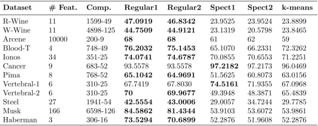
The following datasets were considered (for details about the datasets see [7]): (1) Red Wine (R-Wine) and (2) White Wine (W-Wine), (3) The Arcene dataset (Arcene), (4) The Blood Trans-fusion Dataset (Blood-T), (5) The Ionosphere dataset (Ionos), (6) The Wisconsin Breast cancer dataset (Cancer), (7) The Pima Indian diabetes dataset (Pima), (8) The Vertebral Column dataset (Vertebral-1), the second task (9) (Vertebral-2) is considered as another dataset, (10) The Steel Plates Faults Dataset (Steel), (11) The Musk 2 (Musk) dataset and (12) Haberman’s Survival (Haberman) data.
Next we discuss the metric used for comparison with other clustering algorithms. For evaluating the quality of clustering, we follow the approach of [21] and use the cluster accuracy as a measure. The measure is defined as:
Accuracy= 100∗ Pn i=1δ(yi, map(ci)) n ,
where nis the number of data-points considered, yi represents the true label (ground truth) while
ci is the obtained cluster label of data-point xi. The functionδ(y, c) equals 1 if the true and the
obtained labels match (y =c) and 0 if they don’t. The function mapis basically a permutation function that maps each cluster label to the true label. An optimal match can be found by using the Hungarian Method for the assignment problem [15].
8.2
Case Study
Before reporting comparative results on benchmark datasets, we first consider one dataset as a case study. While experiments reported in this case study were carried on all the benchmark datasets considered, the purpose here is to illustrate the investigations conducted at each stage of application of the regularity lemma. An auxiliary purpose is also to underline a set of guidelines on what changes to the practical regularity partitioning algorithm proved to be useful.
For this task we consider the Red Wine dataset which has 1599 instances with 11 attributes each, the number of classes involved is six. It must be noted though that the class distribution in this dataset is pretty skewed (with the various classes having 10, 53, 681, 638, 199 and 18 datapoints respectively), this makes clustering this dataset quite difficult when k = 6. We however consider both k = 6 and k = 3 to compare results with spectral clustering.
Recall that our method has two meta-parameters that need to be user specified (or estimated by cross-validation): εandl. Note that his usually decided so that it is at least as big as 1
ε. The first
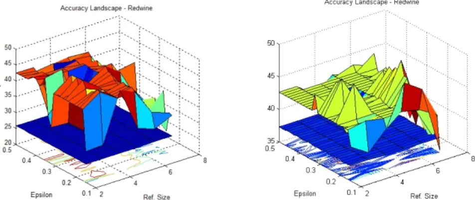
set of experiments thus explore the accuracy landscape of regularity clustering spanned over these two parameters. We consider 25 linearly spaced values ofεbetween 0.15 and 0.50. The refinement number l, as noted in Section 6, can not be too large. Since it can only take integer values, we consider six values from 2 to 7. For the sake of comparison, we also obtain clustering results on the same dataset with spectral clustering with self tuning [22] (both using all connected and k-nearest neighbour graph versions) and k-means clustering. Figure 1 gives the accuracy of the Regularity Clustering on a grid ofεandl. Even though this plot is only for exploratory purposes, it shows that the accuracy landscape is in general much better than the accuracy obtained by spectral clustering for this dataset.
Figure 1: Accuracy Landscape for Regularity Clustering on the Red Wine Dataset for different values of ε and refinement size l (with k = 6 on the left and k = 3 on the right). The Plane cutting through in blue represents accuracy by running self-tuned spectral clustering using the fully connected similarity graph.
Table 1: Reduced Graph Sizes. Original Affinity Matrix size : 1599×1599 ε l 2 3 4 5 6 7 0.15 16×16 27×27 27×27 27×27 36×36 49×49 0.33 49×49 49×49 66×66 66×66 66×66 66×66 0.50 66×66 66×66 66×66 66×66 66×66 66×66
An important aspect of the Regularity Clustering method is that by using a modified constructive version of the Regularity Lemma we obtain a much reduced representation of the original data. The size of the reduced graph depends both onεandl. However, in our observation it is more sensitive to changes to l and understandably so. From the grid for ε and l we take three rows to illustrate the obtained sizes of the reduced graph (more precisely, the dimensions of the affinity matrix of the reduced graph). We compare these numbers with the original dataset size. As we note in the results over the benchmark datasets in section 8.3, this compression is quite big in larger datasets.
The proof of the Regularity Lemma is using a potential function, the index of the partition defined earlier in Definition 3. In each refinement step the index increases significantly. Surprisingly this remains true in our modified refinement algorithm when the number of partition classes is not increasing as fast as in the original version, see Table 2. Another interesting observation is that if we take ε sufficiently high, we do get a regular partition in just a few iterations. A few examples where this was noticed in the Red Wine dataset are mentioned in Table 3.
Finally, before reporting results we must make a comment on constructing the reduced graph. The reduced graph was defined in Definition 5. But note that there is some ambiguity in our case
Table 2: Illustration of Increase in Potential
(ε,l)
ind(P)
ind(P1) ind(P2) ind(P3) ind(P4)
0.15, 2 0.1966 0.2892 0.3321 0.3539
0.33, 2 0.1966 0.2883 0.3321 0.3683
Table 3: Regular Partitions with req. no. of regular pairs and actual no. present (ε,l) # for ε-regularity # of Reg. Pairs # Iterations
0.6, 2 1180 1293 6
0.7, 6 352 391 2
0.7, 7 506 671 2
Table 4: Clustering Results on UCI Datasets. Regular1 and Regular2 represent the results by the versions due to Alon et al. and Frieze-Kannan, respectively. Spect1 and Spect2 give the results for spectral clustering with a k-nearest neighbour graph and a fully connected graph, respectively. Follow the text for more details.
Dataset # Feat. Comp. Regular1 Regular2 Spect1 Spect2 k-means
R-Wine 11 1599-49 47.0919 46.8342 23.9525 23.9524 23.8899 W-Wine 11 4898-125 44.7509 44.9121 23.1319 20.5798 23.8465 Arcene 10000 200-9 68 68 61 62 59 Blood-T 4 748-49 76.2032 75.1453 65.1070 66.2331 72.3262 Ionos 34 351-25 74.0741 74.6787 70.0855 70.6553 71.2251 Cancer 9 683-52 93.5578 93.5578 97.2182 97.2173 96.0469 Pima 8 768-52 65.1042 64.9691 51.5625 60.8073 63.0156 Vertebral-1 6 310-25 67.7419 67.8030 74.5161 71.9355 67.0968 Vertebral-2 6 310-25 70 69.9677 49.3948 48.3871 65.4839 Steel 27 1941-54 42.5554 43.0006 29.0057 34.7244 29.7785 Musk 166 6598-126 84.5862 81.4344 53.9103 53.6072 53.9861 Haberman 3 306-16 73.5294 70.6899 52.2876 51.9608 52.2876
when it comes to constructing the reduced graph. The reduced graph GR is constructed such that
the vertices correspond to the classes in the partition and the edges are associated to theε-regular pairs between classes with density above d. However, in many cases the number of regular pairs is quite small (esp. whenε is small) making the matrix too sparse, making it difficult to find the eigenvectors. Thus for technical reasons we added all pairs to the reduced graph. We contend that this approach works well because the classes that we consider (and thus the densities between them) are obtained after the modified refinement procedure and thus enough information is already embedded in the reduced graph.
8.3
Clustering Results on Benchmark Datasets
In this section we report results on a number of datasets described earlier in Section 8.1. We do a five fold cross-validation on each of the datasets, where a validation set is used to learn the meta-parameters for the data. The accuracy reported is the average clustering quality on the rest of the data after using the learned parameters from the validation set. We use a grid-search to learn the meta-parameters. Initially a coarse grid is initialized with a set of 25 linearly spaced values for ε between 0.15 and 0.50 (we don’t wantεto be outside this range). Forl we simply pick values from 2 to 7 simply because that is the only practical range that we are looking at.
We compare our results with a fixed σ spectral clustering with both a fully connected graph (Spect2) and a k-nearest neighbour graph (Spect1). For the sake of comparison we also include results for k-means on the entire dataset. We also report results on the compression that was achieved on each dataset in Table 4 (The compression is indicated in the format x-y where x represents one
dimension of the adjacency matrix of the dataset and y of the reduced graph).
In the results we observe that the Regularity Clustering method, as indicated by the clustering accuracies is quite powerful; it gave significantly better results in 10 of the 12 datasets. It was also observed that the regularity clustering method did not appear to work very well in synthetic datasets. This seems understandable given the quasi-random aspect of the Regularity method. We also report that the results obtained by the Alon et al. and by the Frieze-Kannan versions are virtually identical, which is not surprising.
9
Future Directions
We believe that this work opens up a lot of potential research problems. First and foremost would be establishing theoretical results for quantifying the approximation obtained by our modifications to the Regularity Lemma. Also, the original Regularity Lemma is applicable only while working with dense graphs. However, there are sparse versions of the Regularity Lemma. These sparse versions could be used in the first phase of our method such that even sparse graphs (k-nearest neighbor graphs) could be used for clustering, thus enhancing its practical utility even further.
A natural generalization of pairwise clustering methods leads to hypergraph partitioning prob-lems [2], [23]. There are a number of results that extend the Regularity Lemma to hypergraphs [3], [9], [17]. It is thus natural that our methodology could be extended to hypergraphs and then used for hypergraph clustering.
In final summary, our work gives a way to harness the Regularity Lemma for the task of clustering. We report results on a number of benchmark datasets which strongly indicate that the method is quite powerful. Based on this work we also suggest a number of possible avenues for future work towards improving and generalizing this methodology.
References
[1] N. Alon, R.A. Duke, H. Lefmann, V. R¨odl, R. Yuster, The Algorithmic Aspects of the Regularity Lemma. In: J. Alg., 16, pp. 80-109, (1994).
[2] S. Bulo, M. Pelillo, A Game-Theoretic Approach to Hypergraph Clustering. In: NIPS, 22, pp. 1571-1579, (2009).
[3] F. Chung, Regularity Lemmas for Hypergraphs and Quasi-randomness. In: Random Struct. Alg., 2, pp. 241-252, (1991).
[4] P. Erd¨os, P. Tur´an, On Some Sequences of Integers. In: J. London Math. Soc, 11, pp. 261-264, (1936).
[5] C. Fowlkes, S. Belongie, F. Chung, J. Malik, Spectral grouping using the Nystr¨om Method. In: IEEE Trans. PAMI, 26, pp. 214-225, (2004).
[6] A. Frieze, R. Kannan, A Simple Algorithm for Constructing Szemer´edi’s Regularity Partition. In: Electron. J. Comb, 6 (1), R17, (1999).
[7] A. Frank, A. Asuncion, UCI Machine Learning Repository, Irvine, CA: University of California, School of Information and Computer Science, (2010).
[8] W.T. Gowers, Lower bounds of tower type for Szemer´edi’s uniformly lemma. In: Geom. Funct. Anal, 7, pp. 322-337, (1997).
[9] W.T. Gowers, Hypergraph regularity and the Multidimensional Szemer´edi theorem, In: Annals of Mathematics, (2) 166 no. 3, pp. 897-946, (2007).
[10] W.T. Gowers, The Work of Endre Szemer´edi, Online athttp://www.abelprize.no/c54147/ binfil/download.php?tid=54060
[11] A. Gy´arf´as, M. Ruszink´o, G.N. S´ark¨ozy, E. Szemer´edi, Three-color Ramsey numbers for paths, In: Combinatorica, 27(1), pp. 35-69, (2007).
[12] Y. Kohayakawa, V. R¨odl, L. Thoma, An optimal algorithm for checking regularity.In: SIAM J. Comput, 32(5), pp. 1210-1235, (2003).
[13] J. Koml´os, G.N. S´ark¨ozy, E. Szemer´edi, Blow-up Lemma, In: Combinatorica, 17(1), pp. 109-123, (1997).
[14] J. Koml´os, A. Shokoufandeh, M. Simonovits, E. Szemer´edi, The Regularity Lemma and Its Applications in Graph Theory. In: Theoretical Aspects of Comp. Sci., LNCS 2292, pp. 84-112, (2002).
[15] H.W. Kuhn, The Hungarian method for the Assignment Problem, In: Naval Research Logistics, 52(1), 2005. Originally appeared in Naval Research Logistics Quarterly, 2, 1955, pp. 83-97.
[16] A. Ng, M. Jordan, Y. Weiss, On Spectral Clustering: Analysis and an algorithm. In T. Diet-terich, S. Becker, and Z. Ghahramani (Eds.),NIPS, MIT Press, 14, pp. 849-856, (2002).
[17] V. R¨odl, B. Nagle, J. Skokan, M. Schacht, Y. Kohayakawa, The Hypergraph Regularity Method and its applications, In: PNAS, 102, pp. 8109-8113, (2005).
[18] S. Shi, J. Malik, Normalized Cuts and Image Segmentation, In: IEEE Trans. PAMI, vol 22, no. 8, pp. 888-905, (2000).
[19] A. Sperotto, M. Pelillo, Szemer´edi’s Regularity Lemma and its Applications to Pairwise Clus-tering and Segmentation. In: EMMCVPR, LNCS 4679. Springer, (2007).
[20] E. Szemer´edi, Regular Partitions of Graphs, Colloques Internationaux C.N.R.S. No 260 -Probl`emes Combinatoires et Th´eorie des Graphes, Orsay, pp. 399-401, (1976).
[21] M. Wu, B. Sch¨olkopf, A Local Learning Approach for Clustering. In: NIPS, pp. 1529-1536, (2007).
[22] L. Zelnik-Manor, P. Perona, Self-tuning Spectral Clustering. In L. K. Saul, Y. Weiss, and L. Bottou, eds., NIPS, MIT Press, Cambridge, MA, pp. 1601-1608, (2005).
[23] D. Zhou, J. Huang, B. Sch¨olkopf, Learning with Hypergraphs: Clustering, Classification, and Embedding. In: NIPS, 19, pp. 16011608, (2007).