Model selection in sparse contingency tables: LASSO penalties vs classical method

Model selection in sparse contingency tables:

LASSO penalties

vs

classical methods

Susana Conde

_{, Gilbert MacKenzie}

1

Behaviour and Health Research Unit, University of Cambridge, Institute of Public Health, Robinson Way, Cambridge CB2 OSR

2

Centre of Biostatistics, Department of Mathematics and Statistics, The Uni-versity of Limerick, Ireland

3

Department of Statistics, School of Mathematical Sciences, Western Gateway Building, Western Road, University College Cork, Ireland

4

CREST, ENSAI, Rennes, France

Abstract: We compare improved classical backward elimination and forward selection methods of model selection in sparse contingency tables with methods based on a regularisation approach involving the least absolute shrinkage and selection operator (LASSO) and the Smooth LASSO. The results show that the modified classical methods outperform the regularisation methods, by producing sparser models which are always hierarchical. Curiously, models selected by the regularisation methods often include effects which are known to be inestimable in the classical paradigm. Our findings support the use of classical methodology.

Keywords:Contingency tables; Model selection; Regularisation, Smooth LASSO; Sparseness.

1

Introduction

Penalized likelihood (Eilers and Marx, 1996) has received a lot of attention recently as a method for achieving smoothness, sparsity, etc. In contin-gency table analysis, Dahinden et al (2007), Park and Hastie (2008), and Conde and MacKenzie (2011) each propose different penalized likelihood approaches. The first of these papers proposes an optimization algorithm using a least absolute shrinkage and selection operator (LASSO) and other penalties while the second develops anL2-norm penalty in a logistic model.

The third paper develops the Smooth LASSO and other LASSO-related penalties. All three approaches are intended to be used in sparse contin-gency tables that can arise from genetic data or multivariate comorbidity data. Such data sets are typically high-dimensional and accordingly pose a major challenge to model selection.

In this paper, we compare model selection methods in sparse contingency tables. Specifically we compare penalized likelihood approaches with our classical stepwise algorithms. The penalized likelihood approaches involve the LASSO with the implementation appeared in Dahinden et al (2007), the LASSO using the Bayes Information Criterion (BIC), which is novel

in this context, and the smooth parametric approximation to the LASSO which appeared in Conde and MacKenzie (2011); the classical algorithms involve modified and enhanced backwards elimination ( MacKenzie-Conde Backwards Elimination (MCBE); Conde, 2011, pp. 137-138, BE2) and for-ward selection (FS).

2

Methods

Let assume the same notation and model of the expected frequencies as in Conde and MacKenzie (2011) i.e. consider ap-dimensional contingency table withq= 2p _{cells, a hierarchical log-linear regression model ln (µ}

i) =

Pk

j=1aijθj with Yates’ constraints where θ is the vector of unknown pa-rameters measuring the influence of constant, main effects and interactions, and all the other quantities as defined in the mentioned paper.

The penalised negative log-likelihood is

−`P(θ, λ) =−`mult(θ) + penλ where pen_λ = λPk

j=2|θj| (LASSO) or penλ = λ

Pk

j=lωln [cosh (θj/ω)] (Smooth LASSO) with ω a certain parameter. We estimate λ using 5-fold cross-validation (CV) and again by BIC. For the smooth (LASSO) we set ω = 1 and use the 95% confidence interval around 0 to determine when a parameter is zero. Note that the LASSO penalty in binary variables coincides with the group-L1norm, which is invariant to the choice of design

matrix. We have that BIC =−2ˆ`+klnnwhere ˆ` is the maximized log-likelihood,kis the number of parameters in the model, andnis the sample size. The algorithms MCBE, BE2, and FS are likelihood-ratio based and work in a stepwise fashion (Conde, 2011, pp. 66-78, 81-85); MCBE starts with the sparse saturated model, that is, the fullest model that can be fitted after eliminating effects with non-existent maximum likelihood estimates detected by MacKenzie’s theorem (Conde, 2011, p. 37-38); BE2 starts with a fitting model with up to and including a certain order of interactions, and FS, with a null (or main effects) model. They remove or add one effect at a time until no other effect can be removed or until they find a model that fits.

When considering 5-fold cross-validation, we selected 20 random samples (i.e. sets of 5 training tables and 5 testing tables). For the LASSO with CV, we used thelogilassopackage in R. For the BIC, we used the same path following algorithm in this package in order to have the estimates of the parameters. In all the penalized likelihood approaches we rescaled the originalλ∈[0,∞), intoλ∗∈[0,1] using the bijective mapping

λ= 1/α[ ln{(1 +λ∗)/(1−λ∗)}] withα= 0.03.

3

Results

We present the results of a small simulation study and then illustrate the methods by analysing some real data from a COPD study of comorbidities (GSK COPD, 2006).

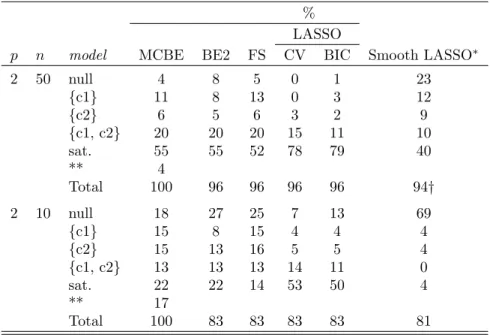
TABLE 1. Percentages of final models found;p= 2, in 100 simulated tables. CV: 5-fold cross-validation. BIC: BIC criterion with a LASSO penalty. The Smooth LASSO approximation is used withω= 1 and 5-fold cross-validation.

% LASSO

p n model MCBE BE2 FS CV BIC Smooth LASSO∗

2 50 null 4 8 5 0 1 23 {c1} 11 8 13 0 3 12 {c2} 6 5 6 3 2 9 {c1, c2} 20 20 20 15 11 10 sat. 55 55 52 78 79 40 ** 4 Total 100 96 96 96 96 94† 2 10 null 18 27 25 7 13 69 {c1} 15 8 15 4 4 4 {c2} 15 13 16 5 5 4 {c1, c2} 13 13 13 14 11 0 sat. 22 22 14 53 50 4 ** 17 Total 100 83 83 83 83 81

∗ _{We removed tables whennlmdid not converge;} (2, 2 respectively in each scenario).

∗∗ _{SSM does not fit.}

3.1 Simulation Study

We simulated 100 2×2 random contingency tables (Conde, 2011, pp. 86-90, 188) and used each of the methods given above to find a final best fitting model.

The sample sizes were n= 50 andn = 10 leading to sparse tables albeit of low dimension - 21% and 79% of the tables have some zero respectively. According to MacKenzie’s theorem (Conde, 2011, pp. 37-39), there are 4

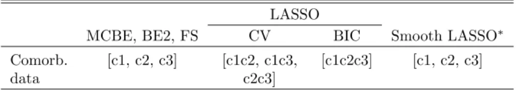
TABLE 2. Final models found with the comorbidity table. Variables mean c1: mild liver disease; c2: diabetes; c3: lung cancer.

LASSO

MCBE, BE2, FS CV BIC Smooth LASSO∗

Comorb. [c1, c2, c3] [c1c2, c1c3, [c1c2c3] [c1, c2, c3]

data c2c3]

∗ _{We removedλ}∗

= 0 from the path asnlmdid not converge.

tables in the first scenario and 22 tables in the second scenario with at least one inestimable effect; these lead to 4 and 17, respectively, tables where the sparse saturated model (SSM) does not fit, as indicated by MCBE, which is the only algorithm of the above that can detect this. We removed the tables whose SSM does not fit from these analyses.

Table 1 presents the results of the simulation study. In all the scenarios studied, the classical stepwise algorithms find sparser, i.e., more parsimo-nious models , and furthermore being in the case of MCBE, free of in-estimable effects models (for example, in the first scenario, all the other algorithms found the saturated model in the four tables whose SSM, which is smaller than the saturated, does not fit. Moreover, none of the penalised likelihood approaches take into account the hierarchical rules for model building.

We note in passing that these tables are simulated at random and we do not know the underlying true models. However, for these scenarios with 2×2 tables, the final models found from any of the classical algorithms can be very reliably taken as the true models (Conde, 2011, pp. 99-100). Fur-thermore, we note that the results are more homogeneous within methods (classical, penalized likelihood) than between methods.

3.2 Real data analysis

As a first step we constructed a three-dimensional contingency table from our comorbidity data, composed by the binary variables: mild liver disease, diabetes, and lung cancer. In Fortran standard order (and the variables in the mentioned order), the table is Y = (45426,20,2568,0,136,0,8,0). We note that according to MacKenzie’s theorem, the maximum likelihood estimates (MLEs) of the effects c1c2, c1c3, and c1c2c3 are nonexistent. Figure 1(a) displays the values of BIC along the path ofλ∗; BIC is minimum in the MLEs.

FIGURE 1. Graphs with comorbidity data and the LASSO penalty. (a) BIC along the path ofλ∗. (b) Values of the MPLEs along the path ofλ∗s. The estimates of λ∗from 5-fold cross-validation and BIC are indistinguishable (and ≈0). For both estimates we used the path following algorithm inlogilassoto maximise the penalised likelihood. The numbers of each line mean 2: c1; 3: c2, . . . , 5: c1c2, 6: c1c3, . . . , 8: c1c2c3.

Table 2 displays the final models found in this table: the three classical algo-rithms and the Smooth LASSO found the main effects model, i.e. conclude that the three comorbidities ar statistically independent. Having lung can-cer is not affected by mild liver disease and diabetes, andvice versawith all the combinations of the three comorbidities. The LASSO, in contrast, found either the all 2-ways model (CV) or the saturated model (BIC) so these approaches would conclude that there is a heavy load of interaction pattern between the comorbidities. Furthermore, the CV and BIC LASSO methods include effects which are formally inestimable in the classical paradigm in their final best fitting models. The Smooth LASSO is more successful, a re-sult which is in agreement with previous findings, perhaps as a consequence of the larger sample size.

Figure 1(b) displays the values of the estimates along the path ofλ∗. The estimates of λ∗ are very close to 0; in the case of the BIC, none of the parameters is zero and in CV, the three-way interaction is 0 (the path of this effect is not monotonic in this case, it is zero for the first λ∗s, then different from 0 untilλ∗ is close to 0.88).

4

Conclusions and discussion

The LASSO penalty is viewed as a method for finding sparse final mod-els. The findings in this paper contradict this overview, whilst comparing LASSO approaches with classical stepwise algorithms in contingency tables. While the methods in thelogilassopackage succeed in some applications (Dahinden and B¨uhlmann, 2009), it is not the case here.

The classical methods outperform all of the penalized likelihood approaches by finding the most parsimonious models which are always hierarchical , and in the case of MCBE, free of inestimable effects as those detected by MacKenzie’s theorem. The results are based on a small simulation but confirm the work carried out in the PhD thesis of the first author.

We have used the Smooth LASSO approximation consideringω= 1 and the use of a normal-based 95% confidence interval to detect a zero parameter. According to the results, it can be considered to be a contender.

Finally, we have alluded to, but not fully discussed, the issue of the nonex-istence of maximum likelihood estimates in sparse tables. Accordingly, we

hope to discuss these points in more detail at the workshop when we will present the results of a more comprehensive simulation study.

References

Conde, S. (2011).Interactions: Log-Linear Models in Sparse Contingency Tables. PhD Thesis. The University of Limerick, Ireland.

Conde, S. and MacKenzie, G. (2008). Search Algorithms for Log-Linear Mod-els in Contingency Tables: Comorbidity Data. In: Proceedings of the 23rd International Workshop on Statistical Modelling, Utrecht, 184-187. Ed.: Eilers, P.H.C.

Conde, S. and MacKenzie, G. (2011). LASSO Penalised Likelihood in High-Dimensional Contingency Tables. In:Proceedings of the 26th International Workshop on Statistical Modelling, Valencia, 127-132. Ed.: Conesa, D. and Forte, A. and L´opez-Qu´ılez, A. and Mu˜noz, F.

Dahinden, C., Parmigiani, G., Emerick, M.C. and B¨uhlmann, P. (2007). Penal-ized likelihood for sparse contingency tables with an application to full-length cDNA libraries.BMC Bioinformatics,8:476.

Dahinden, and B¨uhlmann, P. (2009). Decomposition and Model Selection for Large Contingency Tables.arXiv:0904.1510v2[stat.ME].

Eilers, P.H.C. and Marx, B.D. (1996). Flexible smoothing using B-splines and penalized likelihood (with Comments and Rejoinder). Statistical Science,

11(2)89-121.

Park, M. Y. and Hastie, T. (2008). Penalized logistic regression for detecting gene interactions.Biostatistics,9(1), 30-50.