SHALE: An Efficient Algorithm for Allocation of Guaranteed Display Advertising

Motivated by the problem of optimizing allocation in guaranteed display advertising, we develop an efficient, lightweight method of generating a compactallocation planthat can be used to guide ad server decisions. The plan itself uses justO(1)state per guaranteed contract, is robust to noise, and allows us to serve (provably) nearly optimally. The optimization method we develop is scalable, with a small in-memory footprint, and working in linear time per iteration. It is also “stop-anytime,” meaning that time-critical applications can stop early and still get a good serving solution. Thus, it is particularly useful for optimizing the large problems arising in the context of display advertising. We demonstrate the effectiveness of our algorithm using actual Yahoo! data.

Categories and Subject Descriptors

I.0 [Computing Methodologies]: General

General Terms

Algorithms, Experimentation

Keywords

Display Advertising, Online Advertising

1.

INTRODUCTION

A key problem in display advertising is how to efficiently serve in some (nearly) optimal way. As internet publishers and advertis-ers become increasingly sophisticated, it is not enough to simply make serving choices “correctly” or “acceptably”. Improving ob-jective goals by just a few percent can often improve revenue by

Permission to make digital or hard copies of all or part of this work for personal or classroom use is granted without fee provided that copies are not made or distributed for profit or commercial advantage and that copies bear this notice and the full citation on the first page. To copy otherwise, to republish, to post on servers or to redistribute to lists, requires prior specific permission and/or a fee.

KDD’12,August 12–16, 2012, Beijing, China.

tens of millions of dollars for publishers, as well as improving ad-vertiser or user experience. Serving needs to be done in such a way that we maximize the potential for users, advertisers, and publish-ers.

In this paper, we address serving display advertising in the guar-anteed display marketplace, providing a lightweight optimization framework that allows real servers to allocate ads efficiently and with little overhead. Recall that in guaranteed display advertising, advertisers may target particular types of users visiting particular types of sites over a specified time period. Publishers guarantee to serve their ad some promised number of times to users matching the advertiser’s criteria over the specified duration. We refer to this as acontract.

In [7], the authors show that given a forecast of future inven-tory, it is possible to create an optimalallocation plan, which con-sists of labeling each contract with justO(1)additional informa-tion. Since it is so compact, this allocation plan can efficiently be communicated to ad servers. It requires no online state, which re-moves the need for maintaining immediately accessible impression counts. (Animpressionis generated whenever there is an opportu-nity to display an ad somewhere on a web page for a user.) Given the plan, each ad server can easily decide which ad to serve each impression, even when the impression is one that the forecast never predicted. The delivery produced by following the plan is nearly optimal. Note that simply using an optimizer to find an optimal allocation of contracts to impressions would not produce such a result, since the solution is too large and does not generalize to un-predicted outputs.

The method to generate the allocation plan outlined in [7] relies on the ability to solve large, non-linear optimization problems; it takes as input a bipartite graph representing the set of contracts and a sample of predicted user visits, which can have hundreds of mil-lions of arcs or more. There are commercially available solvers that can be used to create allocation plans. However, they have several drawbacks. The most prominent of these is that such solvers aim towards finding good primal solutions, while the allocation plan generated is not directly tied to the quality of such solutions. (The allocation plan relies on the dual solution of the problem.) In par-ticular, there is no guarantee of how close to optimal the allocation plan really is. Hence, although creating a good allocation plan is

(2)

time critical, stopping the optimizer early with sub-optimal values can have undesirable effects for serving.

For our particular problem, the graph we wish to optimize is ex-tremely large and scalability becomes a real concern. For this rea-son, and given the other disadvantages of using complex third party software, we propose a new solution, called ‘SHALE.’ It addresses all of these concerns, having many desirable properties:

• It has the “stop anytime” property. That is, after complet-ing any iteration, we can stop SHALE and produce a good answer.

• It is a multi-pass streaming algorithm. Each iteration of SHALE runs as a streaming algorithm, reading the arcs off disk one at a time. The total online memory is proportional to the number of contracts and samples used, and is independent of the number of edges in the graph. Because of this, it is pos-sible to handle inputs that are prohibitively large for many commercial solvers without special modifications.

• It is guaranteed to converge to the true optimal solution if it runs for enough iterations. It is robust to sampling, so the input can be generated by sampling rather than using a full input.

• Each contract is annotated with justO(1)information, which can be used to produce nearly optimal serving. Thus, the solution generated creates a practical allocation plan, useable in real serving systems.

The SHALE solver uses the idea of [7] as a starting point, but it provides an additional twist that allows the solver to stop after any number of iterations and still produce a good allocation plan. For this reason, SHALE is often five times faster than solving the full problem using a commercial solver.

1.1

Related Work

The allocation problem facing a display advertising publisher has been the subject of increased attention in the past few years. Often modeled as a special version of a stochastic optimization, several theoretical solutions have been developed [4, 6]. A similar for-mulation of the problem was done by Devanur and Hayes [2],who added an assumption that user arrivals are drawn independently and identically from some distribution, and then proceed to develop al-location plans based on the learned distribution. In contrast, Vee et al. [7] did not assume independence of arrivals, but require the knowledge of the user distributions to formulate the optimization problem.

Bridging the gap between theory and practice, Feldman et al. [3] demonstrated that primal-dual methods can be effective for solv-ing the allocation problem. However, it is not clear how to scale their algorithm to instances on billions of nodes and tens of billions of edges. A different approach was given by Chen et al. [1] who used thestructureof the allocation problem to develop control the-ory based methods to guide the online allocation and mitigate the impact of potential forecast errors.

Finally, a crucial piece of all of the above allocation problems is the underlying optimization function. Ghosh et al [5] define repre-sentative allocations, which minimize the average`22distance

be-tween an allocation given to a specific advertiser, and the ideal one which allocates every eligible impression with equal probability. Feldman et al. [3] define a similar notion offairallocations, which attempt to minimize an`1distance between the achieved allocation

and a similarly defined ideal.

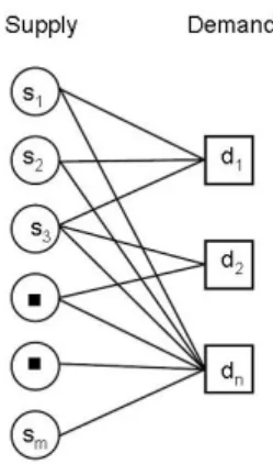
Figure 1: Example bipartite graph

2.

PROBLEM STATEMENT

In this section, we begin by defining the notion of an optimal allocation of ads to users/impressions (Section 2.1). Our goal will then be to serve as close as possible to this optimal allocation. In Section 2.2, we describe the notion of generating an allocation plan, which will be used to produce nearly optimal serving.

2.1

Optimal Allocation

In guaranteed display advertising, we have a large number of forecast impressions together with a number of contracts. These contracts specify ademandas well as a target; we must deliver a number of impressions at least as large as the specified demand, and further, each impression must match the target specified by the contract. We model this as a bipartite graph. On one side are supply nodes, representing impressions. On the other side are de-mand nodes, representing contracts. We add an arc from a given supply node to a given demand node if and only if the impression that the supply node represents iseligible(i.e. matches the target profile) for the contract represented by the demand node. Further, demand nodes are labeled with ademand, which is precisely the amount of impressions guaranteed to the represented contract. In general, supply nodes will represent several impressions each, thus each supply node is labeled with a weightsi, leading to a weighted

graph (see [7] for more details). Figure 1 shows a simple example. An optimal allocation must both be feasible and minimize some objective function. Here, our objective balances two goals: mini-mizing penalty, and maximini-mizingrepresentativeness. Each demand node/contractjhas an associated penalty,pj. Letujbe the

under-delivery, i.e. the number of impressions delivered less thandj.

Then our total penalty isP jpjuj.

Representativeness is a measure of how close our allocation is to some target. For each impressioniand contractj, we define a target, θij. In this paper, we set θij = dj/Sj, whereSj = P

i∈Γ(j)si, the total eligible supply for contractj. This has the

effect of aiming for an equal mix of all possible matching impres-sions. (Here,Γ(j)is the neighborhood ofj, likewise, we denote the neighborhood ofiby Γ(i).) The non-representativeness for contractjis the weightedL2 distance from the targetθijand the

proposed allocation,xij. Specifically, 1 2 X i∈Γ(j) si Vj θij (xij−θij)2,

whereVjis the relative priority of the contractj; a largerVjmeans

that representativeness is more important. Notice that we weight bysito account for the fact that some sample impressions have

(3)

more weight than others. Representativeness is key for advertiser satisfaction. Simply giving an advertiser the least desirable type of users (say, three-year-olds with a history of not spending money) or attempting to serve out an entire contract in a few hours decreases long-term revenue by driving advertisers away. See [5] for more discussion on this idea.

Given these goals, we may write our optimal allocation in terms of a convex optimization problem:

Minimize 1₂P j,i∈Γ(j)si Vj θij(xij−θij) 2 + X j pjuj s.t. P i∈Γ(j)sixij+uj≥dj ∀j (1) P j∈Γ(i)xij≤1 ∀i (2) xij, uj≥0 ∀i, j (3)

Constraints 1 are calleddemand constraints. They guarantee that

ujprecisely represents the total underdelivery to contractj.

Con-straints 2 aresupply constraints, and they specify that we serve no more than one ad for each impression. Constraints 3 are simply non-negativity constraints.

Theoptimal allocationfor the guaranteed display ad problem is the solution to the above problem, where the input bipartite graph represents the full set of contracts and thefull set of impressions! Of course, generating the full set of impressions is impossible in practice. The work of [7] shows that using a sample of impressions still produces an approximately optimal fractional allocation. We interpret the fractions as theprobabilitiesthat a given impression should be allocated to a given contract. Since there are billions of impressions, this leads to serving that is nearly identical.

Although this paper focuses on the above problem, we note that our techniques can be extended to more general objectives. For example, in related work, [8] described a multi-objective model for the allocation of inventory to guaranteed delivery, which combined penalties and representativeness (as above) with revenue made on the non-guaranteed display (NGD) spot market and the potential revenue gained from supplying clicks to contracts. SHALE can easily be extended to handle these variants.

2.2

Compact Serving

In the previous subsection, we defined the notion of optimal al-location. However, serving such an allocation is itself a different problem. Following [7], we define the problem of online serving with forecasts as follows.

We are given as input a bipartite graph, as described in the previ-ous subsection. (We assume this graph is an approximation of the future inventory, although it is not necessary for this definition.) We proceed in two phases.

• Offline Phase: Given the bipartite graph as input, we must

annotate each demand node (corresponding to a contract) withO(1)information. This information will guide the allo-cation during the online phase.

• Online Phase: During the online phase, impressions arrive

one at a time. For each impression, we are given the set of eligible contracts, together with the annotation computed during the offline phase of each returned contract. Using only this information, we must decide which contract to serve to the impression.

Theonline allocationis the actual allocation of impressions to con-tracts given during the online phase. Our goal is to produce an online allocation that is as close to optimal as possible.

Remarkably, the work of [1] shows that there is an algorithm that solves the above problem nearly optimally. If the input bipartite graph exactly models the future impressions, then the online allo-cation produced is optimal. If the input bipartite graph is generated by sampling from the future, then the online allocation produced is provably approximately optimal.

However, the previous work simply assumed that an optimal so-lution can be found during the Offline Phase. Although this is true, it does not address many of the practical concerns that come with solving large-scale non-linear optimization problems. In the fol-lowing sections, we describe our solution, which in addition to solving the problem of compact serving, is fast, simple, and robust.

3.

ALGORITHMS

3.1

Plan creation using full solution

The proposal of [7] to create an allocation plan was to solve the problem of Section 2.1 using standard methods. From this, we can compute theduals of the problem. In particular, we may write the problem in terms of its Lagrangian (more formally, we use the KKT conditions). Every constraint then has a corresponding dual variable. (Intuitively, the harder a constraint is to satisfy, the larger its dual variable in the optimal solution.)

The allocation plan then consists of the demand duals of the problem, denotedα. So each contractjwas labeled with the de-mand dual from the corresponding dede-mand constraint,αj. The

supply duals, denotedβ, and the non-negativity duals were simply thrown out.

A key insight of this earlier work is that we can reconstruct the optimal solution using only theαvalues. When impressioni ar-rives, the value ofβican be found online by solving the equation P

j∈Γ(i)gij(αj −βi) = 1, resettingβi = 0if the solution is

less than 0. Here,gij(z) = max{0, θij(1 +z/Vj)}. We then set xij=gij(αj−βi)for eachj∈Γ(i). Somewhat surprisingly, this

yields an optimal allocation. (And when the value ofαis obtained by solving a sampled problem, it is approximately optimal.)

As mentioned in the introduction, although this solution has many nice properties, solving the optimization problem using standard methods is slower than desirable. Thus, we have a need for faster methods.

3.2

Greedy solution (HWM)

An alternate approach to solving the allocation problem is the High Water Mark(HWM) algorithm, based on a greedy heuristic. This method first orders all the contracts by theirallocation order. Here, the allocation order puts contracts with smallerSj(i.e. total

eligible supply) before contracts with largerSj. Then, the

algo-rithm goes through each contract one after another, trying to allo-cate an equal fraction from all the eligible ad opportunities. This fraction is denotedζfor each contract, and corresponds roughly to its demand dual. Contractjis given fractionζjfrom each eligible

impression,unlessprevious contracts have taken more than a1−ζj

fraction already. In this case, contractjgets whatever fraction is left (possibly 0).

If there is very little contention (or contractjcomes early in the allocation order), thenζj=dj/Sj. This will give exactly the right

amount of inventory to contractj. However, if a lot of inventory has already been allocated whenjis processed, itsζjvalue may be

larger than this to accommodate the fact that it gets less thanζjfor

some impressions. Settingζ = 1will give a contract all inventory that has not already been allocated. We do this in the case that there is not enough remaining inventory to satisfy the demand ofj.

(4)

1. Order all demand nodes in decreasing contention order (dj/Sj).

2. For each supply nodei, initialize the available weights˜i = si.

3. For each demand nodej, in allocation order: (a) Findζjsuch that

X

i∈Bj

min{s˜i, ζjsi}=dj,

settingζj=∞if the above has no solution.

(b) For each matching supply nodesi∈Bj

Updates˜i= ˜si−min{s˜i, ζjsi}.

We note that the computation in Step 3a can be done in time linear in the size of|Bj|. Hence, the total runtime of the HWM algorithm

is linear in the number of arcs in the graph.

3.3

SHALE

Obtaining a full solution using traditional methods is too slow (and more precise than needed), while the HWM heuristic, although very fast, sacrifices optimality. SHALE is a method that spans the two approaches. If it runs for enough iterations, it produces the true optimal solution. Running it for 0 iterations (plus an additional step at the end) produces the HWM allocation. So we can easily balance precision with running time. In our experience (see Sec-tion 4), just 10 or 20 iteraSec-tions of SHALE yield remarkably good results; for serving, even using 5 iterations works quite well since forecast errors and other issues generally dwarf small variations in the solution. Further, SHALE is amenable to “warm-starts,” using the previous allocation plan as a starting point. In this case, it is even better.

SHALE is based on the solution using optimal duals. The key innovation, however, is the ability to takeany dual solution and convert it into a good primal solution. We do this by extending the simple heuristic HWM to incorporate dual values. Thus, the SHALE algorithm has two pieces. The first piece finds reasonable duals. This piece is an iterative algorithm. On each iteration, the dual solution will generally improve. (And repeated iterations con-verge to the true optimal.) The second piece converts the reasonable set of duals we found (more precisely, theαvalues, as described earlier) into a good primal solution.

The optimization for SHALE relies heavily on the machinery provided by the KKT conditions. Interested readers may find a more detailed discussion in the Appendix. Here, we note the fol-lowing. Ifα∗andβ∗are optimal dual values, then

1. The optimal primal solution is given byx∗ij=gij(α∗j−β

∗

i),

wheregij(z) = max{0, θij(1 +z/Vj)}.

2. For all j, 0 ≤ α∗j ≤ pj. Further, either α∗j = pj or P

i∈Γ(j)six

∗

ij=dj.

3. For alli,βi≥0. Further, eitherβi= 0orPj∈Γ(i)x

∗

ij= 1.

The pseudo-code for SHALE is shown below.

• Initialize. Setαj= 0for allj.

• Stage One. Repeat until we run out of time:

1. For each impressioni, findβithat satisfies X

j∈Γ(i)

gij(αj−βi) = 1

Ifβi<0or no solution exists, updateβi= 0.

2. For each contractj, findαjthat satisfies X

i∈Γ(j)

sigij(αj−βi) =dj

Ifαj> pjor no solution exists, updateαj=pj.

• Stage Two.

1. Initializes˜i= 1for alli.

2. For each impressioni, findβithat satisfies X

j∈Γ(i)

gij(αj−βi) = 1

Ifβi<0or no solution exists, updateβi= 0.

3. For each contractj, in allocation order, do: (a) Findζjthat satisfies

X

i∈Γ(j)

min{˜si, sigij(ζj−βi)}=dj,

settingζj=∞if there is no solution.

(b) For each impressionieligible forj, updates˜i = ˜

si−min{s˜i, sigij(ζj−βi)}.

• OutputTheαjandζjvalues for eachj.

Our implementation of SHALE runs in linear time (in the num-ber of arcs in the input graph) per iteration.

During Stage One, we iteratively improve theαvalues by assum-ing that theβvalues are correct and solving the equation forα. Re-call thatxij=gij(αj−βi). Thus, we are simply solving the

equa-tionP

i∈Γ(j)sixij =djforαj. In order to find betterβvalues,

we assume theαis correct and solve forβusingP

j∈Γ(i)xij= 1.

The following theorem shows that this simple iterative technique converges, and yields anεapproximation in polynomial steps.

More precisely, definedj(α) =P_i∈Γ(j)sigij(αj−βi), where

βis determined as in Step 1 of Stage One of SHALE. (We think of this as the projected delivery for contractjusing only Stage One of SHALE.) We say a givenαsolution produces anε-approximate deliveryif for allj, eitherαj =pjordj(α) ≥(1−ε)dj. Note

that an optimalαjis at mostpj; the intuitive reason for this is that

growingαjany larger will cause the non-representativeness of the

contract’s delivery to be even more costly than the under-delivery penalty. Thus, anε-approximate delivery means that every contract is projected to deliver withinεof the desired amount, or itsαjis

“maxed-out.”

We can now state our theorem. Its proof is in the appendix. THEOREM 1. Stage One of SHALE converges to the optimal solution of the guaranteed display allocation problem. Further, let

ε > 0. Then within 1_εnmaxj{pj/Vj}iterations, the outputα

produces anε-approximate delivery.

Note that Stage One is effectively a form of coordinate descent. In general, it could be replaced with any standard optimization technique that allows us to recover a set of approximate dual val-ues. However, the form we use is simple to understand, use, and debug. Further, it works very well in practice.

In Stage Two, we calculateζvalues in a way similar to HWM. We calculateβvalues based on theαvalues generated from Stage One. Using these, we calculateζ values to givedjallocation (if

possible) to each contract. Notice that in Stage Two, we must be cognizant of the actual allocation. Thus, we maintain a remaining fraction left,˜si, that we cannot exceed. Thus, contracts allocated

(5)

latest may not be able to get the full amount specified bygij, if the

fraction taken from impressioniis too great.

We note that in our actual implementation, we use a two-pass version of Stage Two. In the first pass, we boundζjbyαjfor each j. In the second pass, we find a second set ofζ values (with no upper bounds), utilizing any left-over inventory. This is somewhat “truer” to the allocation produced by SHALE in Stage One, and gives slightly better online allocation.

3.3.1

Online Serving with SHALE

Recall that SHALE produces two values for each contractj, namelyαjandζj. Given impressioni, theαvalues for eligible

contracts are used to calculate theβivalue, which is used together

with the ζvalues to produce the allocation. The pseudo-code is below.

Input:Impressioniand the set of eligible contracts.

1. Set˜si= 1and findβisuch that X

j∈Γ(i)

gij(αj−βi) = 1

Ifβi<0or no solution exists, setβi= 0.

2. For each matching contractj, in allocation order, compute

xij= min{s˜i, gij(ζi−βi)}and updates˜i←˜si−xij.

3. Select contractjwith probabilityxij. (IfP_j_Γ(_i₎xij < 1,

then there is some chance that no contract is selected.)

4.

EXPERIMENTS

We have implemented both the HWM and SHALE algorithms described in Section 3 and benchmarked their performance against the full solution approach (known hereafter as XPRESS) on his-torical booked contract sets. First we describe these datasets and our chosen performance metrics and then present our evaluation results.

4.1

Experimental setup

In order to test the “real-world” performance of all three algo-rithms we considered 6 sets of real GD contracts booked and active in the recent past. In particular, we chose three periods of time as described in Table 1 and two ad positions LREC and SKY for each of these time periods.

Contracts Contracts Booked before Active between

11/16/09 11/16/09 - 11/30/09 01/03/10 01/03/10 - 01/17/10 04/13/10 04/13/10 - 04/20/10

Table 1: Contract Time Periods

We considered US region contracts booked to the aforementioned positions and time periods and also excluded all frequency capped contracts and all contracts with time-of-day and other custom tar-gets. Also, all remaining contracts that were active for longer than the specified date ranges were truncated and their demands were proportionally reduced. Next, we generated a bipartite graph for each contract set as in Figure 1; by sampling50eligible impres-sions for each contract in the set. This sampling procedure is de-scribed in detail in [7]. We then ran HWM, SHALE and XPRESS on each of the 6 graphs and evaluated the following metrics.

1. Under-delivery Rate: This represents the total under-delivered

impressions as a proportion of the booked demand, i.e.,

U = P juj P jdj (4)

2. Penalty Cost: This represents the penalty incurred by the

publisher for failing to deliver the guaranteed number of im-pressions to booked GD contracts. Note that the true long-term penalty due to under-delivery is not known since we cannot easily forecast how an advertiser’s future business with the publisher will change due to under-delivery on a booked contract. Here we define the total penalty cost to be

P = X j

pjuj (5)

whereuj is the number of under-delivered impressions to

contractjandpjis the cost for each under-delivered

impres-sion. For our experiments, we setpjto bepj= 0.005 + qj

whereqjis the revenue per delivered impression from

con-tractj. Indeed, it is intuitive and reasonable to expect that contracts that are more valuable to the advertiser incur larger penalties for under-delivery. The offset (here$5CP M) serves to ensure that our algorithms attempt to fully deliver even the contracts with low booking prices.

3. L2 Distance: This metric shows how much the generated

allocation deviates from a desired allocation (for example a perfectly representative one). In particular, the L2 distance is the non-representativeness function1₂P

i∈Γ(j)si

Vj

θij(xij−

θij)2, the first term of the objective function in Section 2,

corresponding to the weighted`2

2distance between target and

allocation.

4.2

Experiment 1

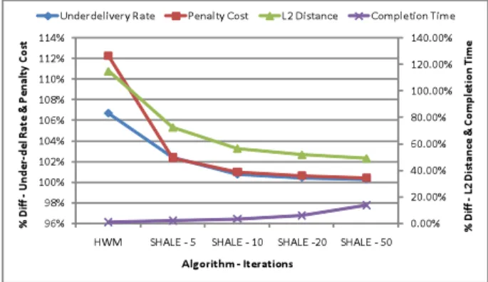
As we mentioned earlier, SHALE was designed to provide a trade-off between the speed of execution of HWM and the quality of solutions output by XPRESS. Accordingly in our first experi-ment we measured the performance of SHALE (run for 0, 5, 10, 20 and 50 iterations) as compared to XPRESS against our chosen met-rics. Since SHALE at 0 iterations is the same as HWM, we label it as such. Figure 2 shows the penalty cost, under-delivery rate, L2

Figure 2: Performance Vs. Completion time

distance and completion for HWM and SHALE run for 5, 10, 20 and 50 iterations respectively as a percentage of the corresponding metric for XPRESS, averaged over our 6 chosen contract sets. Note that the y-axis labels for the under-delivery rate and penalty cost are on the left, while the labels for the L2 distance and completion time are on the right.

(6)

It is immediately clear that SHALE after only 10 iterations is within 2% of XPRESS with respect to penalty cost and under-delivery rate. Further, note that SHALE after 10 iterations is able to provide an allocation whose L2 distance is less than half that of XPRESS. (Recall smaller L2 distance means the solution is more representative, so SHALE is doing twice as well on this metric.) Remarkably, SHALE is able to generate a high quality solution while requiring less than 20% of the time taken by XPRESS.

4.3

Experiment 2

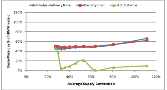
Next, we decided to fix the iteration count for SHALE at 20 and test its performance under varying supply levels. Specifically, for each of our 6 contract sets, we artificially reduced the supply weight on each of the supply nodes while keeping the graph structure fixed in order to simulate the increasing scarcity of supply. We define the average supply contention (ASC) metric to represent the scarcity of supply, as follows ASC = P isi P j∈i dj Sj P isi (6) wheresirepresents the supply weight anddjandSjrepresent the

demand and eligible supply for contractj. In Figure 3, we show the under-delivery rate, penalty cost and L2 distance for SHALE as a percentage of the corresponding metric for HWM for various levels of ASC. First we note that each of our metrics for SHALE is lower

Figure 3: SHALE Vs. HWM

than the corresponding metric for HWM for all values of ASC. In-deed, the SHALE L2 distance is less than 50% of that for HWM. Also note that the SHALE penalty cost consistently improves com-pared to HWM as the ASC increases.

4.4

Experiment 3

Recall that the allocation plan produced by SHALE or HWM in production is expected to be used not on the input graph itself but on real impressions as they arrive. Thus, the graph on which the primal solution is reconstructed could potentially be very different from the sampled graph used for optimization. Whereas a “true” test of SHALE in production is out of the scope of this work, we did compare the robustness of SHALE (run for 20 iterations) and HWM by reconstructing the allocation plan generated be each al-gorithm on graphs different from those used for optimization. In particular, corresponding to each of our 6 contract sets, we first ran SHALE and HWM on corresponding 50 sample graphs to gener-ate allocation plans. Then, for each contract set, we genergener-ated 6 different 200 sample graphs using 6 different random seeds. We also varied the ASC in the same fashion as in Experiment 2 in each

of these 6 graphs. We then reconstructed primal solutions from the plans generated by HWM and SHALE on these graphs and evaluated our chosen metrics. Figure 4 shows the comparison of

Figure 4: SHALE Vs. HWM reconstructed

under-delivery rate, penalty cost and L2 distance for SHALE as a percentage of the corresponding metric for HWM averaged over 36 graphs (6 different contract sets and 6 graphs for each contract set) for various values of ASC. Here, we can clearly see that SHALE performs significantly better than HWM on all three metrics. It turns out that the HWM allocation plan resulted in much higher under-delivery rates, penalty costs and L2 distances when recon-structed on the new 200 sample graphs as compared to the primal solution on the original 50 sample graph; whereas the SHALE allo-cation plan did not suffer such a degradation in the solution quality upon reconstruction on the 200 sample graphs. Finally, note that the L2 distance ratio, unlike penalty cost and under-delivery date is not monotonic in the ASC. We would like to point out that in fact, the L2 distance for SHALE was monotonically increasing in the ASC; whereas the L2 distance for HWM varied erratically. This caused the SHALE L2 distance as a percentage of the HWM L2 distance to be non-monotonic.

4.5

Experiment 4

The experiments above compare how SHALE performs with re-spect to the optimal algorithm under knowledge of supply land-scape of the contracts. In this experiment we compare how these algorithms perform when the solution is used to serve real world sampled impressions from actual server logs. This experiment uses real contracts and real adserver logs (downsampled) for performing the complete offline simulation.

4.5.1

Setup

Here we take three new datasets which consists of real guaran-teed delivery contracts from Yahoo! active during different one to two week periods in the past year. We run our optimization al-gorithms and serve real downsampled serving logs for two hours using the solution computed. Then after collecting the serving stats we reoptimize the contracts with updated goal and supply forecasts as the contract demands would have reduced after two hours of serving. This cycle continues where we optimize, serve adlogs and update stats every two hour for the entire test period of one two two weeks.

4.5.2

Algorithms compared

At the end of the simulation, we look at the contracts that start and end within the simulation period and compare how metrics of under delivery and penalty across HWM, SHALE and "Optimal"

(7)

algorithms. HWM algorithm is essentially SHALE algorithm with 0 iterations. The SHALE algorithms are run with setting of 5, 10 and 20 iterations. Here the "Optimal" solution is obtained by run-ning a coordinate gradient descent algorithm till the objective func-tion convergence.

We performed serving using the reconstruction algorithm de-scribed in Section 3.3.1.

4.5.3

Metrics

The metrics include the underdelivery metric and penalty metrics as defined in Equation 4 and in Equation 5 For these set of experi-ments, we setpjto bepj= 0.002 + 4∗qjwhereqjis the revenue

per delivered impression from contractj.

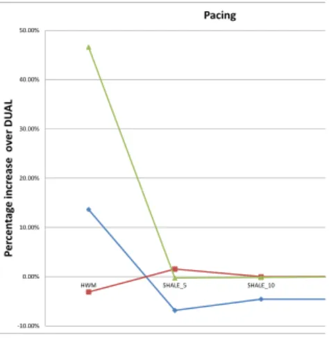
We also compare another metric called pacing between these al-gorithms. This captures how representative contracts are with re-spect to time dimension while delivering these contracts. Pacing is defined as the percentage of contracts that are within 12% of the linear delivery goal atleast 80% of their active duration.

4.5.4

Results

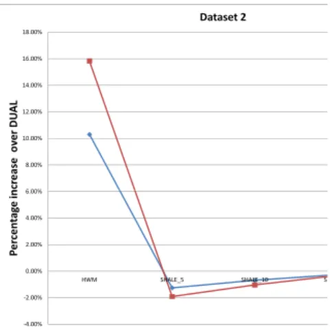
Figures 5, 6 and 7 show that the under delivery and penalty cost for HWM (SHALE with 0 iterations) algorithm is the worst. Fur-ther as the number of SHALE iterations increase it gets very close to the "Optimal" algorithm. Note that even SHALE with 5 or 10 iterations performs as good or sometimes slightly better than the "Optimal" algorithm. This can be attributed to different reasons; one being the fact that there are forecasting errors intrinsic to using real serving logs. The other reason might be the fact that the ob-jective function of "Optimal" algorithm is not just optimizing for these two metrics.

0.00% 0.20% 0.40% 0.60% 0.80% 1.00% 1.20% 1.40% 1.60%

HWM SHALE_5 SHALE_10 SHALE_20

P e rc e n tag e i n cr e as e o v e r D U A L Dataset 1 UnderDelivery Penalty Cost

Figure 5: Dataset 1: Under Delivery and Penalty Cost Compar-ison

Figure 8 shows how these algorithm perform with respect to pac-ing. The pacing is pretty similar for all three datasets SHALE with 5, 10 and 20 iterations when compared with "Optimal" algorithm but HWM has better pacing than SHALE and "Optimal" for the other two datasets. The possible reasons here can be that SHALE and "Optimal" algorithm gives better under delivery and penalty cost compromising some pacing. Also note that time dimension is just one of the possible dimensions for the representativeness part f the objective function and SHALE and "Optimal" algorithm opti-mizes for all possible dimensions.

6.00% 8.00% 10.00% 12.00% 14.00% 16.00% 18.00% P e rc e n tag e i n cr e as e o v e r D U A L Dataset 2 UnderDelivery Penalty Cost -4.00% -2.00% 0.00% 2.00% 4.00% 6.00%

HWM SHALE_5 SHALE_10 SHALE_20

P e rc e n tag e i n cr e as e o v e r D U A L

Figure 6: Dataset 2: Under Delivery and Penalty Cost Compar-ison 0.00% 1.00% 2.00% 3.00% 4.00% 5.00% P e rc e n tag e i n cr e as e o v e r D U A L Dataset 3 UnderDelivery Penalty Cost -4.00% -3.00% -2.00% -1.00% 0.00%

HWM SHALE_5 SHALE_10 SHALE_20

P e rc e n tag e i n cr e as e o v e r D U A L

Figure 7: Dataset 3: Under Delivery and Penalty Cost Compar-ison

5.

CONCLUSION

We described the SHALE algorithm, which is used to generate compact allocation plans leading to near-optimal serving. Our al-gorithm is scalable, efficient, and has the stop-anytime property, making it particularly useful in time-sensitive applications. Our ex-periments demonstrate that it is many times faster than using com-mercially available general purpose solvers, while still leading to near-optimal solutions. On the other side, it produces a much bet-ter and more robust solution than the simple HWM heuristic. Due to its stop-anytime property, it can be configured to give the de-sired tradeoff between running time and optimality of the solution. Furthermore, SHALE can handle “warm starts,” using a previous allocation plan as a starting point for future iterations.

SHALE is easily modified to handle additional goals, such as maximizing revenue in the non-guaranteed market or click-through rate of advertisement. In fact, the technique appears to be amenable to other classes of problems involving many users with supply

(8)

con-20.00% 30.00% 40.00% 50.00% P e rc e n tag e i n cr e as e o v e r D U A L Pacing Dataset 1 Dataset 2 Dataset 3 -10.00% 0.00% 10.00%

HWM SHALE_5 SHALE_10 SHALE_20

P e rc e n tag e i n cr e as e o v e r D U A L Dataset 3

Figure 8: Pacing Comparisons on all three datasets

straints (e.g. each user is shown only one item). Thus, although SHALE is particularly well-suited to optimizing guaranteed display ad delivery, it is also an effective lightweight optimizer. It can han-dle huge, memory-intensive inputs, and the underlying techniques we use provide a useful method of mapping non-optimal dual solu-tions into nearly optimal primal results.

6.

ADDITIONAL AUTHORS

7.

REFERENCES

[1] Y. Chen, P. Berkhin, B. Anderson, and N. R. Devanur. Real-time bidding algorithms for performance-based display ad allocation. In C. Apté, J. Ghosh, and P. Smyth, editors, KDD, pages 1307–1315. ACM, 2011.

[2] N. R. Devenur and T. P. Hayes. The adwords problem: online keyword matching with budgeted bidders under random permutations. In J. Chuang, L. Fortnow, and P. Pu, editors, ACM Conference on Electronic Commerce, pages 71–78. ACM, 2009.

[3] J. Feldman, M. Henzinger, N. Korula, V. S. Mirrokni, and C. Stein. Online stochastic packing applied to display ad allocation. In M. de Berg and U. Meyer, editors,ESA (1), volume 6346 ofLecture Notes in Computer Science, pages 182–194. Springer, 2010.

[4] J. Feldman, A. Mehta, V. S. Mirrokni, and S. Muthukrishnan. Online stochastic matching: Beating 1-1/e. InFOCS, pages 117–126. IEEE Computer Society, 2009.

[5] A. Ghosh, P. McAfee, K. Papineni, and S. Vassilvitskii. Bidding for representative allocations for display advertising. In S. Leonardi, editor,WINE, volume 5929 ofLecture Notes in Computer Science, pages 208–219. Springer, 2009. [6] V. S. Mirrokni, S. O. Gharan, and M. Zadimoghaddam.

Simultaneous approximations for adversarial and stochastic online budgeted allocation. In D. Randall, editor,SODA, pages 1690–1701. SIAM, 2012.

[7] E. Vee, S. Vassilvitskii, and J. Shanmugasundaram. Optimal online assignment with forecasts. In D. C. Parkes,

C. Dellarocas, and M. Tennenholtz, editors,ACM Conference on Electronic Commerce, pages 109–118. ACM, 2010.

[8] J. Yang, E. Vee, S. Vassilvitskii, J. Tomlin,

J. Shanmugasundaram, T. Anastasakos, and O. Kennedy. Inventory allocation for online graphical display advertising. CoRR, abs/1008.3551, 2010.

Appendix

Recall that our optimization problem is Minimize 1₂P j,i∈Γ(j)si Vj θij(xij−θij) 2 + X j pjuj s.t. P i∈Γ(j)sixij+uj≥dj ∀j (7) siP_j_∈_Γ(_i₎xij≤si ∀i (8) xij, uj≥0 ∀i, j (9)

Notice that we have multiplied the supply constraints bysito aid

our mathematics later.

The KKT conditions generalize the somewhat more familiar La-grangian. Letαjdenote the demand duals. Letβidenote the

sup-ply duals. Letγijdenote the non-negativity duals forxij, and let ψj denote the non-negativity dual foruj. For our problem, the

KKT conditions tell us the optimal primal-dual solution must sat-isfy the following

Stationarity: For alli, j, si Vj θij (xij−θij)−siαj+siβi−γij For alli, pj−αj−ψj= 0 Complementary slackness:

For allj, eitherαj= 0orP_i∈Γ(j)sixij+uj=dj.

For alli, eitherβi= 0orP_j∈Γ(i)sixij=si.

For alli, j, eitherγij= 0orxij= 0.

For allj, eitherψj= 0oruj= 0.

The dual feasibity conditions also tell us thatαj ≥ 0,βi ≥ 0, γij ≥ 0, andψj ≥ 0for alli, j. (While the primal feasibility

conditions tell us that the constraints in the original problem must be satified.) Since our objective is convex, and primal-dual solution satisfying the KKT conditions is in fact optimal.

Notice that the stationarity conditions are effectively like taking the derivative of the Lagrangian. The first of these tells us that

xij=θij(1 +

αj−βi+γij/si Vj

)

The complementary slackness condition for the γij tells us that γij = 0unlessxij = 0. This has the effect that when the

ex-pressionθij(1 + αj−βi

Vj )is negative,γijwill increase just enough

to makexij= 0. In particular, this implies xij= max{0, θij(1 +

αj−βi Vj

)}=gij(αj−βi)

The second stationarity condition shows αj = pj −ψj. Since ψj ≥0, this immediately shows thatαj ≤pj. Further, the

com-plementary slackness condition forψjimplies thatψ = 0unless uj= 0. That is, eitherαj=pjorP_i∈Γ(j)sixij≥dj. By

com-plementary slackness ofαj, we see in fact that equality must hold

(i.e. P

i∈Γ(j)sixij=dj) unlessαj = 0. But whenαj= 0,

in-spection reveals thatP

i∈Γ(j)sixij=

P

i∈Γ(j)sigij(−βi)≤dj.

(9)

Finally, the complementary slackness condition onβi implies

eitherβi= 0orP_j_∈_Γ(_i₎xij= 1. Putting all of this together, we

see that

1. The optimal primal solution is given byx∗ij=gij(α∗j−βi∗),

wheregij(z) = max{0, θij(1 +z/Vj)}.

2. For allj,0≤α∗j≤pj. Further, eitherα∗j=pjor P

i∈Γ(j)six∗ij=dj.

3. For alli,βi≥0. Further, eitherβi= 0orPj∈Γ(i)x

∗

ij= 1.

as we claimed in Section 3.

PROOF OFTHEOREM1. First, note that αj is bounded above

bypj. We will show thatαjis non-decreasing on each iteration.

Letαtrefer to the value of alpha computed during thet-th iteration, whereα0j = 0for allj. We show by induction thatdj(αt)≤dj

for allt≥0. The base case follows by definition, sinceβi≥0for

alli:dj(α0)≤Pi∈Γ(j)sigij(0−0) =Pi∈Γ(j)siθij=dj.

So assume for somet≥0thatdj(αt)≤djfor allj. Letβtbe

the value computed in Step 1 of Stage One of SHALE, givenαt. We see that dj(αt) = X i∈Γ(j) sigij(αtj−β t i) = X i∈Γ(j) simax{0, θij(1 + αtj−βit Vj )}

Further, by the way in which αt+1 is calculated (in Stage One, Step 2), we have thatαt_j+1must either bepjor satisfy the

follow-ing: dj= X i∈Γ(j) sigij(αtj+1−β t i) = X i∈Γ(j) simax{0, θij(1 + αt+1 j −β t i Vj )}

Using the fact that for any numbers a ≥ b that max{0, a} −

max{0, b} ≤ a−b(which can be shown by an easy case anal-ysis), we have dj−dj(αt) = X i∈Γ(j) simax{0, θij(1 + αtj+1−β t i Vj )} − X i∈Γ(j) simax{0, θij(1 + αtj−βit Vj )} ≤ X i∈Γ(j) siθij(αtj+1−α t j)/Vj =dj(αtj+1−α t j)/Vj

That is, eitherαt_j+1=pjor αtj+1=α t j+Vj(1− dj(αt) dj ) (10)

Sincedj(αt)≤djby assumption, this shows thatαtj+1≥α t jfor

eachj. We must still prove thatdj(αt+1)≤dj. To this end, note

that theβt+1generated in Step 1 for the givenαt+1must greater than or equal toβt , sinceαt+1_≥_αt . That is,βt+1 i ≥β t ifor alli. Thus, dj(αt+1) = X i∈Γ(j) simax{0, θij(1 + αt_j+1−β_it+1 Vj )} ≤ X i∈Γ(j) simax{0, θij(1 + αtj+1−β t i Vj )} =dj as we wanted.

In general, we can use the fact thatdj(αt)≤djfor allt, together

with Equation 10, to see that theαjvalues are non-decreasing at

each iteration. From this (together with the fact thatαjis bounded

bypj), it immediately follows that the algorithm converges.

To see that the algorithm converges to the optimal solution, we note that the dual values generated by SHALE satisfy the KKT conditions at convergence: for allj, eitherαj=pjordj(α) =dj

(i.e.pj−αj−ψj= 0with eitherψj= 0oruj= 0), with similar

arguments holding for the other duals. Since the problem we study is convex, this shows that the primal solution generated must be the optimal.

As for our second claim, suppose that there is somejfor which

αtj6=pjbutdj(αtj)≤(1−ε)dj. Then by Equation 10, we see αtj+1=α t j+Vj(1− dj(αt) dj )≥αtj+Vjε

That is,αt_j+1increases (overαjt) by at leastεVj. Sinceαtjstarts

at 0, is bounded bypj, and never decreases, we see that this can

happen at mostpj/(εVj)times for eachj. In this worst case, this