Comparing selfh healing techniques in approximate MAC accelerators

(1)

January 27, 2019

BACHELOR ASSIGNMENT

K. Raben s1568426

Faculty of Electrical Engineering, Mathematics and Computer Science (EEMCS) Computer Architecture for Embedded Systems

Exam committee:

G.A. Gillani, A. B. J. Kokkeler, M.S. Oude Alink

COMPARING

SELF-HEALING TECHNIQUES IN

APPROXIMATE MAC

(2)

Abstract

Approximate computing is the technique of trading in accuracy for efficiency in calculations. This efficiency can come in many forms such as reduction in used hardware area or reduced power consump-tion. To even further these methods, circuits can be designed that introduce self-healing, where some portion of the reduced accuracy can get internally compensated by letting different errors cancel each other out. One of these circuits is a Multiply Accumulate (MAC) circuit, where a multiplication is made and then added to the total result.

(3)

1 Introduction

Approximate computing is the technique of computing with a smaller degree of precision which creates opportunities for improving systems in terms of used area, power consumption and performance efficiency. This technique can be uti-lized in applications which can tolerate approximation errors and will still out-put information that is useful. Examples of these applications are deep learning networks, machine learning, web searches and image and video processing[1].

To increase efficiency even further, error balancing can be introduced in cer-tain structures that will reduce the average error of these structures. One of these structures is a Multiply-Accumulate Circuit (MAC), which is often used in radio astronomy[2].

A MAC calculates the dot product of two input vectors, meaning that every element of vector−→A gets multiplied with the corresponding element of vector

− →

[image:5.612.200.409.341.390.2]

B and the results get added up, as illustrated by Fig. 1.

Figure 1: MAC block diagram[3]

When building a MAC with approximate multipliers, there is a chance that the multiplier will make an error, sayδm. Thisδmcan however be compensated

in the accumulator stage if another error was made with the same magnitude, only with a different sign, i.e.,−δm.

Using this compensating ability, configurations for a MAC can be found that have lower measures of error than when using conventional approximate com-puting techniques while still using the same amount of resources.

Different techniques utilizing this Self-Healing ability have been developed. One technique focuses on balancing the error internally by configuring the multiplier in such a way that the produced errors can be healed[4]. The other technique uses an additional ”mirror” multiplier that balances the first multiplier[5]. In this work, the goal is to answer the question: What approximate multiplier technique using an FPGA is best when used in accumulation based accelerators? A model is build to evaluate approximate multiplier configurations. The model outputs results for different quality metrics and an estimation for the resource costs. This work will discuss the subjects of approximate multipliers and Self-Healing techniques more extensively and will show the method for creating the model and obtaining the parameters used in it.

(6)

2 Background

2.1 Approximate Multipliers

[image:6.612.226.387.228.342.2]

One can create a multiplier of n×n-bits by constructing it using multiple elemen-tary 2×2 multipliers. The realization of an accurate 2×2 multiplier in hardware can be found in Fig. 2. The corresponding truth table of Fig. 2 can be found in Fig. 3.

Figure 2: Accurate 2×2-bit multiplier

Figure 3: Truth table of an accurate 2×2 multiplier[3]

Using four of these multipliers and some adder logic a 4×4-bit multiplier can be build. The functioning of the logic can be seen in Fig. 4. The 4-bit inputs get divided into two 2-bit elements, after which every possible 2-bit multiplication is made. Adding these partial products with Shifting the products of the more significant bits as shown in Fig. 4 will conclude in an 8-bit result of the 4×4-bit multiplier.

This same process can be repeated to create a 8×8-bit multiplier using four 4-bit multipliers, a 16×16-bit multiplier with four 8-bit multipliers etc.

[image:6.612.222.392.387.459.2]

(7)

[image:7.612.218.397.137.235.2]

Figure 4: Design of a 4×4-bit multiplier[5]

Figure 5: Approximate multiplier M2[4]

been generated[4]. Conventional approximate computing builds bigger multipli-ers out of these elemental multiplimultipli-ers to create systems that have a certain error probability but where the gains in hardware area and power consumption make up for this sacrifice.

When using approximate elementary 2×2 multipliers inside of a larger mul-tiplier like an 8×8 multiplier a certain error is introduced. Important to note is that the significance of that error is dependant on where the elementary 2×2 multiplier is placed in the larger multiplier. In Fig. 6 the functioning of an 8×8 multiplier build from elementary 2×2 multipliers can be seen. In an×n

multiplier, wherenalways is a power of 2, there aren2_/_{4 elementary 2}_×₂

mul-tipliers needed. In the case of a 4×4 multiplier like in Fig. 4 that results in 4 elementary multipliers, and in the case of a 8×8 multiplier like in Fig. 6, 16 elementary multipliers are used. The outputO8×8of the 8×8 multiplier is given

in Eq.(1), from which it can be seen how significant a certain multiplier, and the possible error made, is to the end result.

[image:7.612.224.389.278.366.2]

(8)

[image:8.612.178.431.122.307.2]

Figure 6: A 8×8-bit Multiplier Using 2×2-bit multiplier elements[5].

O8×8= 4096(AHHBHH)

+ 1024(AHLBHH+AHHBHL)

+ 256(AHLBHL+AHHBLH+ALHBHH)

+ 64(AHHBLL+AHLBLH+ALHBHL+ALLBHH)

+ 16(ALLBHL+AHLBLL+ALHBLH)

+ 4(ALHBLL+ALLBLH)

+ALLBLL

(1)

From this the mean error of a conventional approximate multiplier can be described as in Eq.(2), whereiis one of the 2×2 multipliers,Siis the shift factor

of that multiplier,Eiis the error magnitude that can occur with that multiplier

andP(Ei) is the probability that an error will occur in that multiplier.

EM U L=

n2/4

X

i=1

|(Si∗Ei∗P(E)i)| (2)

(9)

are handled. After this the MAC will output a single number. This output of a MAC is given in Eq.(3). HereM is the number of elements in the input vectors andAmandBmare themth elements of the input vectors

− →

A and−→B.

OM AC= − →

A·−→B =

M

X

m=1

(Am∗Bm) (3)

Using the field of approximate computing both stages can be reduced in cost by using approximate multipliers and approximate adders. This work solely focuses on the implementation of approximate multipliers in a MAC and all used adders in this work are accurate.

2.3 Self-Healing Techniques

Using an approximate multiplier, the quality of the result is decreased in sacrifice for a more efficient circuit. In case of a MAC, errors will start to accumulate and the output will start to deviate from the accurate answer. The mean error of a MAC is described in Eq.(4).

EM AC =

M

X

m=1

EM U L

=

M

X

m=1

n2_/₄

X

i=1

(Si∗Ei∗P(E)i)

=M

n2_/₄

X

i=1

(Si∗Ei∗P(E)i)

(4)

An important aspect to note is that the absolute value is taken after the summation of all the multiplications, which differs from Eq.(2) for just a mul-tiplier. This is because the accumulation stage offers an opportunity to reduce the total error made by a MAC[4]. This Self-Healing effect occurs when the multiplier stage makes errors with opposing signs, which then can cancel (part of) another error in the accumulator stage. To achieve this effect, more types of approximate elementary 2×2-bit multipliers need to be used. For instance for the multiplier M2, which makes the error 3×3 = 7 the multiplier M3 from [4] can be introduced, which makes the error 3×3 = 11 and thus has an error of +2 that can balance the -2 error of M2. The circuit for M3 and the corresponding truth table can be found in Fig. 7.

2.3.1 Internal Self-Healing

Using multiple elementary approximate multipliers with opposing errors a cir-cuit can be build that can achieve the Self-Healing effect. One option proposed

(10)

[image:10.612.137.472.133.224.2]

(a) Circuit Layout (b) Truth Table

Figure 7: Approximate multiplier M3[4] and the corresponding truth table[5]

by [5] is to configure a larger multiplier to use both types of elementary multi-pliers inside of its multiplication stage. The created multiplier stage will then functions as is described in Fig. 8, where both errors of magnitude +δand−δ

will occur, which will cancel each other in the accumulator stage.

Figure 8: Internal Self-Healing methodology[5]

For example, looking at Fig. 6 again, if the multiplier ALH∗BLL is set to

use M2 (which has an error magnitude of -2) andALL∗BLH is set to use M3

(which has an error magnitude of +2), the errors can cancel each other once the results get accumulated. In a situation where the input vectors would have infinite elements that are uniformly distributed, Eq.(5) would then hold, where the mean error of the MAC becomes zero since the sum of the multiplier errors becomes zero.

EM AC =M

n2_/₄

X

i=1

(Si∗Ei∗P(E)i)

= 0

[image:10.612.170.442.325.419.2]

(11)

2.3.2 Mirror Self-Healing

The technique suggested in [4] proposes to instead of balancing the error in one multiplier internally, an additional multiplier is constructed which produces the same error, but with an opposite sign. When the results of the approximate multiplier and the ”mirror” multiplier are added by the accumulator section,

errors would be canceled. The technique is also described in Fig. 9. The

mathematical description of the error for this technique is given in Eq.(6), where

[image:11.612.191.423.249.337.2]

iandjare the different elementary 2×2 multipliers in the two larger multipliers.

Figure 9: Mirror Self-Healing methodology[5]

EM AC =

M/2

X

m=1

EM U L1+EM U L2

EM AC =

M/2

X

m=1

 

n2_/₄

X

i=1

(Si∗Ei∗P(E)i) + n2_/₄

X

j=1

(Sj∗Ej∗P(E)j)

 

=M

2

 

n2_/₄

X

i=1

(Si∗Ei∗P(E)i) + n2_/₄

X

j=1

(Sj∗Ej∗P(E)j)

 

(6)

In the case when the input vectors would have infinite elements that are uniformly distributed, Eq.(7 would hold whereEM U L1would converge toδand

EM U L2would converge to−δ, which would result in the total mean error of the

MAC to reduce to zero.

EM U L1=

n2/4

X

i=1

(Si∗Ei∗P(E)i) = +δ

EM U L2=

n2/4

X

j=1

(Sj∗ −Ej∗P(E)j) =−δ

=⇒ EM AC =δ−δ

= 0

(7)

(12)

Since two multipliers are used, the resources needed for the multiplier stage doubles in comparison with the internal self-healing technique. However, since the elements of the input vectors are divided over the two multipliers the throughput is also doubled, resulting in the same performance as two internal self-healing MACs in parallel.

2.4 Error Analysis

To analyze the two self-healing techniques there are different measures for qual-ity that can be used. A straightforward error metric is the mean error which is given in Eq.(8) whereOacc(n) is thekth accurate output of a MAC andOapp(n)

the approximate output.

ME = 1

K

X

k=1

|Oacc(k)−Oapp(k)| (8)

Another commonly used error metric is the Mean Squared Error (MSE). Because of the square the MSE is less forgiving to larger errors than it is to smaller errors resulting in more distinction between different designs. The MSE is calculated as given in Eq.(9).

MSE = 1

K

X

k=1

(Oacc(k)−Oapp(k))2 (9)

A problem with the mean error and mean squared error is that the outcome highly depends on how large the results from the MAC are. A MAC which uses an input vector of 200 elements with a uniform distribution will have a much smaller output than a MAC which uses an input vector of 1000 elements with that same distribution. To be able to still compare these results, another error metric is introduced, the mean percentage error.

The mean percentage error (MPE) is calculated as shown in Eq.(10). Since every error is divided by the accurate result the size of the result is compensated for.

MPE = 100∗ 1

K

X

k=1

|Oacc(k)−Oapp(k)|

Oacc(k)

(13)

3 Method

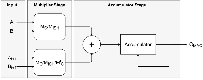
To be able to compare the different techniques, they are evaluated in the same setup. The conventional approximation technique, the internal self-healing tech-nique and the mirror self-healing techtech-nique are implemented in a MAC with 2 multipliers in the multiplier stage, the results of these multiplications are added and given to the accumulator. This setup can be seen in Fig. 10. Where the techniques differ in setup is in the configurations of the multipliers. For both the conventional approximate computing methodology (Where approxi-mate multipliers are used without a possibility for error balancing) and the internal self-healing methodology the two multipliers will use the exact same configurations, Mc and MISH in Fig. 10. The mirror self-healing

methodol-ogy however will have one multiplier configured with multipliers used by the conventional methodology (Mc) and will mirror that multiplier in the second

multiplier used(M_c0). Using this setup, all techniques will use the same amount of multipliers.

MC/MISH

MC/MISH/M

'

C

+

Accumulator

A_i Bi

Ai+1

Bi+1

OMAC

[image:13.612.141.471.326.456.2]

Input Multiplier Stage Accumulator Stage

Figure 10: MAC design under evaluation

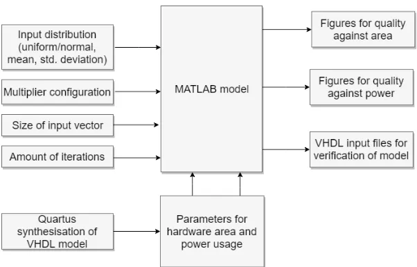
To evaluate the techniques, a model is build in MATLAB that outputs fig-ures for quality against hardware area and quality against power usage for a certain chosen multiplier configuration. A block diagram of the functioning of the model is given in Fig. 11. The model computes these figures for quality from parameters given as input, such as the chosen input distribution, the amount of elements in the input vector and the configuration of the elementary multipli-ers. From these inputs the model computes an estimation for the used hardware area and power consumption for FPGA, based on parameters synthesized by the Quartus tooling and quality metrics as described in section 2.4 are calculated.

(14)

[image:14.612.155.456.121.314.2]

Figure 11: Block overview of the used MATLAB model

3.1 Multiplier Creation

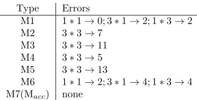
For this work a total of seven multiplier designs are used, one accurate and six approximate. The error cases of these designs can be seen in Table 1. The circuits and corresponding truth tables can be found in appendix A. M1[7] is a multiplier with three error cases of magnitude -1, M2[6] is the multiplier al-ready described in section 2.1. These two multipliers are often used for building conventional approximate multipliers, where there is no error balancing. M3 is introduced by [4] as a mirror multiplier for M2 as discussed in section 2.3. M4 is the multiplier introduced by [5] to compensate the bit overflow in adders that M3 can cause.

(15)

Type Errors

M1 1∗1→0; 3∗1→2; 1∗3→2

M2 3∗3→7

M3 3∗3→11

M4 3∗3→5

M5 3∗3→13

M6 1∗1→2; 3∗1→4; 1∗3→4

[image:15.612.208.402.122.220.2]

M7(Macc) none

Table 1: Elementary 2×2 multipliers used

3.2 Overflow in the multiplier

When introducing approximate circuits which can have a higher maximum result than the accurate case, like M3 and M5, the problem arises that within a larger multiplier (build of these elementary 2×2 multipliers) overflow can occur. For instance if a 4×4 multiplier is build using only the M3 multiplier, the maximum output that can occur is 275, which exceeds the maximum for an 8-bit number, which is 255. Therefore this should be taken into account when picking designs as designs that overflow are not usable.

3.3 Design Space Exploration

To see which self-healing technique functions better, the best configurations for these techniques are needed. To find these configurations the design space ex-ploration algorithm from [5] is used. This algorithm will evaluate every possible configuration from a given set of multiplier types and will output the Pareto op-timal configurations that have the smallest mean error as calculated by Eq.(2)

for a given area or power consumption. The algorithm can calculate these

Pareto optimal configurations for conventional approximate multipliers and for approximate multipliers that use the internal self-healing technique. The algo-rithm also computes if a configuration will have the possibility to overflow, and if so, it will discard that configuration.

3.4 Cost Analysis using Quartus

To get figures for the cost in hardware area and power consumption on an FPGA the Quartus tooling is used. The VHDL code can be found in appendix B. This VHDL code is largely based on the work of [3], where the code for a MAC with configurable multipliers was already created. The addition made to this code enables it to synthesize a configurable MAC with two 8×8 multipliers comply-ing to the mirror self-healcomply-ing methodology. The Register Transfer Level (RTL) view of the synthesis can be seen in appendix C. Another addition is the code for the newly created multipliers from section 3.1.

The outcomes of these simulations are discussed in section 4. From these out-comes for hardware area and power consumption parameters are obtained that

(16)

are used in the MATLAB model to create cost estimations for multiplier con-figurations.

3.4.1 Area Calculation

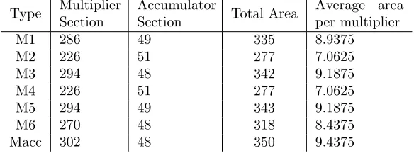
In Table 2 the hardware area costs are shown for an FPGA of the Cyclone IV E family, EP4CE115F29C8. To find the hardware area for all the types of mul-tipliers used in the MATLAB model, a MAC is synthesized that always uses a multiplier section consisting of 2 8-bit multipliers. This means that in total 32 elementary 2×2 multipliers are used. The area used by the larger multipliers consists of combinational logic and adders. Synthesis optimizes the resource usage of the setup and therefore is not always using exactly the same amount of logic cells, which is the hardware building block of an FPGA, for every elemen-tary multiplier. To compensate for this deviation an 8-bit MAC is synthesized which uses only 1 type of multiplier. From the area report of that MAC the amount of logic cells used for the accumulator section is subtracted, leaving the amount of logic cells used by the 2 multipliers. This number is divided by 32 to conclude the value for 1 multiplier. In this value the accompanying adder logic is also taken into account. The areas are also shown for the accumulator section. For the MATLAB model an average of all the accumulator areas is used as a parameter.

Type Multiplier

Section

Accumulator

Section Total Area

Average area

per multiplier

M1 286 49 335 8.9375

M2 226 51 277 7.0625

M3 294 48 342 9.1875

M4 226 51 277 7.0625

M5 294 49 343 9.1875

M6 270 48 318 8.4375

[image:16.612.160.452.386.494.2]

Macc 302 48 350 9.4375

Table 2: Hardware area of different multiplier types expressed in logic cells

3.4.2 Power Analysis

(17)

vector with 496 elements or 4960 elements and a uniform or normal input dis-tribution with mean 128 and a standard deviation of 40. The clock speed is set to 50 MHz, which came close to the maximum clock speed Quartus indicated was possible for this circuit on this FPGA. The results for power usage with the different input vectors can be found in appendix E. In Table 3 the results are shown which were computed with an input vector of 4960 elements, uniformly distributed. The results shown are the dynamic power consumption numbers as computed by Quartus, meaning that these results report on the power con-sumption caused by switching activities of the circuit when it is performing calculations. Therefore certain aspects like static power consumption to keep the FPGA running are not taken into account, which gives us a clearer view on the functioning of the circuit configuration.

Type Multiplier

Section

Accumulator Section

Total Dynamic Power

Average Power per Multiplier

M1 1.33 1.15 2.48 0.04156

M2 1.26 1.09 2.35 0.03938

M3 1.52 1.10 2.62 0.04750

M4 1.46 1.19 2.65 0.04563

M5 1.52 1.24 2.76 0.04750

M6 1.38 1.18 2.56 0.04313

[image:17.612.161.454.280.400.2]

Macc 1.51 1.23 2.74 0.04719

Table 3: Power usage (in mW) of different multiplier types, computed with an input vector of 4960 uniformly distributed elements.

From these results a few observations are made. When comparing the results for different input distributions in appendix E it can be seen that the difference between results obtained from uniform and normal distributions is minimal. The consistency in the results holds not only in case of a uniform or normal distribution, but also for the different input sizes. The deviation in power usage between different types of multipliers tends to be bigger than the deviation in power usage between the different sizes of input vectors, which can be seen as a positive indication for the accuracy of the results.

Another observation is that unlike the situation for area, the influence of the accumulator section on the total result is much higher for the case of power usage. For example, the accumulator section for M1 in terms of hardware area takes up 14.6% of the total area. In the case of power, the dynamic power usage of the accumulator section of M1 takes up 46% of the total dynamic power usage of the MAC.

(18)

3.5 MATLAB Model

The MATLAB model calculates the quality of a MAC configuration and plots that quality against the hardware area or power usage of that configuration. The code for the entire model can be found in appendix D.

3.5.1 Error Analysis

(19)

Algorithm 1Pseudo-code for quality evaluation

Input:

VecAmount: The amount of input vectors that are made, increasing this number increases the accuracy of the result.

VecSize: The amount of elements in the input vectors.

Config: The configuration of the elementary multipliers in the MAC, given in a matrix with one configuration on every row.

InputType: Whether the configuration should be evaluated with a uni-form or normal input distribution.

Mean: The mean to use when evaluating with a normal distribution.

Dev: The standard deviation to use when evaluating with a normal dis-tribution.

Mirrored: Whether the MAC uses the mirror Self-Healing methodology or not.

Variables:

Area: Vector with the hardware area costs calculated by the model for every configuration.

Power: Vector with the power usage costs calculated by the model for every configuration.

Input: Variable to store the created inputs.

App Result: Vector that accumulates the outputs of the approximate multiplier.

Acc Result: Vector that accumulates the outputs of the accurate multi-plier.

1: fori ={1,...,rows(Config)}do

2: Area(i) = CalculateArea(Config row(i),Mirrored)

3: Power(i) = CalculatePower(Config row(i),Mirrored)

4: forj = {1,...,VecAmount}do

5: if InputType = ’Uniform’then

6: Input = CreateUniformInput(VecSize)

7: else

8: if InputType = ’Normal’then

9: Input = CreateNormalInput(VecSize, Mean, Dev)

10: End if

11: fork ={1,...,VecSize}do

12: App Result(j) = App Result(j) +

13: App Multiplication(Config row(i), Input(k),Mirrored)

14: Acc Result(j) = Acc Result(j) + Acc Multiplication(Input(k))

15: End for

16: End for

17: ME(i) = Calculalte ME(App Result, Acc Result)

18: MPE(i) = Calculalte MPE(App Result, Acc Result)

19: MSE(i) = Calculalte MSE(App Result, Acc Result)

20: End for

21: Plot(ME, MPE, MSE, Area)

22: Plot(ME, MPE, MSE, Power)

(20)

3.5.2 Input Creation

The quality of an approximate multiplier is dependant on the distribution of the input it receives. Uniform and normal distributed inputs are created to evaluate a MAC on how it behaves in different circumstances since the input vectors in practical situations will often have a certain distribution. This can highly effect the performance of a MAC since different multipliers handle different sections of the input numbers. For instance looking at Fig. 6 again, if a normal distribution is used with a mean of 128, the probability that a multiplier calculating the highest significance multiplication, soAHH ∗BHH, will have to multiply 3∗3

is very slim. Making it less prone to errors if an approximate multiplier is used in that position.

For the creation of input vectors the model uses the function randi and

randn, where randi creates random uniformly distributed integers in a certain

number range andrandncreates standard normal distributed random numbers.

The standard normal distribution has a mean of 0 and a standard deviation of 1. These random numbers are multiplied by the desired standard deviation given as input to the model and shifted to create a distribution that has a mean value as that specified as input. Sincerandndoes not output integers, but only integer values are used in the system, the numbers are rounded to the nearest integer. Any value that is out of the range of the multiplier is rounded to either 2n _{for an}_n_{-bits multiplier, or to 0, depending on what side the number is out of}

(21)

[image:21.612.138.473.133.232.2]

(a) Uniform Distribution (b) Normal Distribution

Figure 12: Distribution of input vectors with 248 elements to simulate radio astronomy applications [1]

3.6 Model Verification

To ensure the validity of the created MATLAB model, verification using Mod-elsim is performed. The MATLAB model can output automatically generated VHDL, code where input vectors created by the MATLAB model are written down. This VHDL testbench file is then opened in Modelsim and executed on the VHDL model of the MAC. This way, the MATLAB model and the model in Modelsim will receive the exact same inputs. The output of Modelsim is then compared to that of MATLAB to verify it behaves in the same way.

(22)

4 Results

4.1 Area and power of 2

×

2 multipliers

[image:22.612.167.445.227.379.2]

Through Quartus synthesis results are found for the amount of hardware area used by the different multipliers in a MAC setup. A table of the results is already shown in section 3.4.1. These average area results are also graphically displayed in Fig. 13.

Figure 13: Area in logic cells of different multiplier types

These results show that all constructed multipliers use a smaller amount of logic cells in comparison with the accurate multiplier with M2 and M4 standing out as having the lowest area. M3, M5 and M6 use a significantly larger area, but are used as mirror pairs for other multipliers and therefore are still relevant. The mirror pair of M1 and M6 are different in that the circuit produces a low error magnitude but with a higher error frequency and therefore interesting as comparison to the other circuits which have a high error magnitude but a low error rate.

(23)

[image:23.612.167.444.123.277.2]

Figure 14: Power in mW of different multiplier types

4.2 Error Analysis of Self-Healing Configurations

Using the created MATLAB model several configurations are evaluated. Pareto optimal configurations are found using the design space exploration algorithm designed by [5]. This algorithm outputs configurations for conventional approx-imate multipliers and configurations for the Internal Self-Healing methodology. On the configurations for the conventional approximate multiplier the mirror self-healing methodology is applied and thus every approximate multiplier is mirrored. For example, if a conventional configuration for a 4×4 multiplier would be [M2,M2,M1,M4], the configuration for the mirror multiplier would then be [M3,M3,M6,M5]. This results in configurations for the three methodol-ogy’s: Conventional, Internal Self-Healing and Mirror Self-Healing.

The elementary multiplier parameters found by the Quartus synthesis as discussed in section 4.1 are implemented into the algorithm. Configurations are found that have the lowest analytic mean error for either hardware area or power consumption. Configurations are either optimized for a uniform distribution or a normal distribution. The resulted configurations can be found in appendix F. The results of the quality evaluation for all the evaluated configurations can be found in appendix H. In this section, a selection of these plots are discussed. In Fig. 15 an enlarged graph can be seen of a single result plot. This graph shows the results for Pareto optimal configurations computed for the least area and using a uniform input. The vector size in this case is 4960.

Overflow configurations

A very important thing to note in Fig. 15 is that many designs of the mirror self-healing technique will cause an overflow. In the graph the distinction is made between designs that overflow (black) and designs that do not (magenta). These overflow designs are caused by the fact that the mirror self-healing tech-nique exactly mirrors the conventional healing configurations. The conventional healing technique can use multiplier types M1, M2 and the accurate multiplier. But since the M1 multiplier is using significantly more resources than M2 the

(24)

270 280 290 300 310 320 330 340 350 10-5

10-4

10-3

10-2

10-1

100

101

MPE (%)

Uniform distribution

Conventional Pareto Optimal Internal SH Pareto Optimal Mirror SH (Overflow) Mirror SH

[image:24.612.161.449.128.283.2]

Area (LC)

Figure 15: Results optimized for area and uniform input distribution

Pareto optimal configurations use only M2 and the accurate multiplier. This re-sults in that the mirror self-healing configurations use only M3 and the accurate multiplier, and creates many cases where there are too many M3 multipliers in one 4×4 multiplier creating the possibility for overflow as described in section 3.2. To remedy this problem for these configurations it is possible to switch certain elementary multipliers between the two large multipliers. For instance if a certain 4×4 multiplier in the conventional setup uses only M2 multipliers and thus the mirrored 4×4 multiplier uses only M3 multipliers, one can switch the most significant elementary multiplier, resulting in 1 multiplier that uses the configuration [M3,M2,M2,M2] and one that uses [M2,M3,M3,M3] and both 4×4 multipliers will not be able to overflow. The result of a system with those configurations does not change in comparison. Doing this however is deviating from the methodology as proposed in [4]. Another option to gain more insight of the mirror self-healing methodology is to create a design space exploration specifically for the mirror self-healing technique, which would also filter out designs that overflow.

minimal cost for mirror self-healing technique

(25)

mean error as described in Eq.(2) in section 2.1 for a certain area. This means that as soon as a multiplier configuration is fully balanced it has mean error = 0. In Fig. 15 this is the point where the internal self-healing (blue) line stops. The mirror self-healing however always achieves this mean error = 0, since every conventional approximate multiplier will get mirrored.

In Fig. 16 the results are shown not for Pareto optimal configurations, but for configurations where the mean error as described in Eq.(2) is always 0. I.e., every approximate multiplier will get mirrored with another multiplier with the same significance. The configurations shown are increasing in approximation and use only the multipliers M2, M3 and the accurate multiplier. The exact configu-rations can be found in appendix G. In this case it is clearly visible that the mirror self-healing technique is superior to the internal self-healing technique. The reason for this is that with the mirror technique absolute self-healing can already happen with the least significant multiplier (multiplierALL∗BLLin Fig.

6). This gives the mirror technique an advantage as it can gain the same area reduction as the internal self-healing technique, but can place the approximate multipliers on lower significant places.

305 310 315 320 325 330 335 340 345 350

Area (LC)

10-4 10-3 10-2

10-1

100

MPE (%)

[image:25.612.157.449.347.499.2]

Internal SH Mirror SH

Figure 16: Results for configuration with increasing approximation, Vector size: 496

Difference in Area and Power Fig. 17 shows the same circumstances as

Fig. 15, only using configurations optimized for power usage. From comparing these two figures it can be seen that the results for area and power are quite alike in shape, and also the found Pareto optimal configurations do not differ drastically. The main cause for this is that like in the results for area, multiplier M2 still is the most efficient for power and is therefore used a lot.

The significance of the vector size

In Fig. 18 the results can be seen as computed for different vector sizes. The vector sizes are 496, 496∗4 and 496∗10 elements. It can be clearly seen that with the increase of the vector size, the effectiveness of both the self-healing

(26)

270 280 290 300 310 320 330 340 350 Power (mW)

10-5 10-4

10-3 10-2

10-1

100 101

MPE (%)

Conventional Pareto Optimal

Internal SH Pareto Optimal

[image:26.612.159.448.128.284.2]

Mirror SH

Figure 17: Results optimized for Power and uniform input distribution

(27)

270 280 290 300 310 320 330 340 350

Area (LC)

10-5 10-4 10-3 10-2 10-1 100 101

MPE (%)

Conventional Pareto Optimal Internal SH Pareto Optimal Mirror SH

(a) Vector Size: 496

270 280 290 300 310 320 330 340 350

Area (LC)

10-5 10-4 10-3 10-2 10-1 100 101

MPE (%)

(b) Vector Size: 1984

270 280 290 300 310 320 330 340 350

Area (LC)

10-5 10-4 10-3 10-2 10-1 100 101

MPE (%)

[image:27.612.175.435.123.478.2]

(c) Vector Size: 4960

Figure 18: MPE results for different vector sizes with a uniform distribution

(28)

5 Conclusion

In this work, two different techniques for self-healing in a MAC applied on an FPGA have been compared. From the results in section 4 can be seen that al-though both techniques have their advantages, the mirror self-healing technique as described in [4] comes with a lot of restrictions. To start, the technique is only usable in cases where there is already a need for 2 MACs to be used in parallel, otherwise using this technique would already almost double the hardware area needed. Second, the chance of a mirrored multiplier to have the possibility to overflow is quite high, rendering a lot of configurations unusable if applying the exact methodology of mirroring a conventional approximate multiplier. Third, because of this method of always mirroring, the minimal hardware cost that can be achieved by this technique is relatively high. An advantage that the mirror self-healing technique possesses is the ability to balance errors with using only the lowest significant multipliers. However, in general the quality of the results produced by the mirroring technique are not able to compensate for the restric-tions it has.

(29)

6 Discussion

Evaluating the results questions arise that were not addressed in the time per-mitted. These subjects are treated below.

Cost results for FPGA

In section 4.1 the hardware costs of a MAC on an FPGA are discussed. From these results it became apparent that the costs for multipliers on FPGA do not correspond that well with those for ASIC as discussed in [4] and [5]. For exam-ple, the newly created multiplier M6 has a lower area cost than that of multiplier M3, but uses far more gates if it would be build in ASIC and therefore use more hardware area.

Overflow in the multipliers

As discussed in section 4.2 a lot of the found configurations using the mirror self-healing technique are able to overflow. This problem arises because the design space exploration used is build for finding Pareto optimal configurations for the conventional and internal self-healing techniques without overflow cases. Using the conventional configurations and mirroring them is the technique as described in [4]. However, this technique is build for a Square Accumulator (SAC) and within a SAC bit overflow is a much smaller problem since a SAC utilizes a number of 2×2 squarers which compensate for overflow. Using this exact same technique on a MAC therefore is much harder. The technique can however be adjusted, as discussed in theoverflow configurationspart of section 4.2.

Comparing the different self-healing techniques

When comparing the internal self-healing technique and the mirror self-healing technique the problem arises that the mirror self-healing methodology is severely limited in area reduction by the fact that every approximate multiplier should be mirrored. This increases the minimal hardware costs when using this technique and can more easily result in configurations with bit overflow.

(30)

7 Future Work

In the field of approximate computing there is still a lot of room for future investigations, focusing on the subjects treated in this work, the following items are still worth investigating:

• As mentioned in section 6, optimization for FPGA can still improve a

great deal. The conventional methodology uses certain approximate mul-tipliers because they use less gates and therefore make less hardware cost, which makes sense when working in a ASIC environment. For an FPGA environment however, it does not, and further investigation could be done on which multiplier setups are more efficient for FPGA. This was out of scope for this work, since the goal is to compare the self-healing techniques as they were presented.

• The mirror self-healing technique is severely limited in performance since the methodology restricts itself to only exactly mirror a conventional mul-tiplier, creating problems like bit overflow and a high minimal resource cost. In future work, an adjusted methodology could be developed that works around these restrictions by not simply mirroring the conventional multiplier, but adjust both multipliers in a way that the multipliers bal-ance each other but do not overflow.

• Since the design space exploration algorithm used in this work only com-puted the Pareto optimal configurations for the conventional technique and the internal self-healing technique, not all possible mirror self-healing options are evaluated and overflow cases are not filtered out. In future work, the design space exploration algorithm could be expanded to also consider mirror self-healing configurations, which will allow a better com-parison between the different techniques.

(31)

References

[1] M. Shafique, R. Hafiz, S. Rehman, W. El-Harouni and J. Henkel, ”Invited: Cross-layer approximate computing: From logic to architectures,” 2016 53nd ACM/EDAC/IEEE Design Automation Conference (DAC), Austin, TX, 2016, pp. 1-6.

[2] L. D’Addario and D. Wang. ”An integrated circuit for radio astronomy cor-relators supporting large arrays of antennas,” Journal of Astronomical In-strumentation, 2016.

[3] B. Verstoep. ”Approximate multipliers for MAC,” Bachelor assignment, Uni-versity of Twente, Faculty of Electrical Engineering, Mathematics and Com-puter Science, April 2018.

[4] G. A. Gillani, M. A. Hanif, M. Krone, S. H. Gerez, M. Shafique, and A. B. J. Kokkeler, ”Squash: Approximate Square-Accumulate With Self-Healing,” IEEE Access, 6, 49112-49128. 2018.

[5] G. A. Gillani et al. ”MACISH: Designing Approximate MAC Accelerators with Internal-Self-Healing,” [Still to be published] 2019.

[6] P. Kulkarni, P. Gupta, M. Ercegovac, “Trading Accuracy for Power with an Underdesigned Multiplier Architecture,” 24th International Conference on VLSI Design (VLSI Design), pp. 346 – 351, 2011.

[7] Semeen Rehman, Walaa El-Harouni, Muhammad Shafique, Akash Kumar, and Jorg Henkel, ”Architectural-space exploration of approximate multipli-ers,” In Frank Liu, editor, ICCAD, page 80. ACM, 2016.

[8] A. Marcovitz. ”The Karnaugh Map,” in Introduction to Logic Design,

McGraw-Hill, 2009, pp. 111-199.

[9] S. Gerez. ”Power Analysis with Quartus II and Modelsim,” University of Twente, Faculty of Electrical Engineering, Mathematics and Computer Sci-ence, March 2015.

(32)

Appendices

A

Multiplier Circuits and Truth Tables

(a) Circuit M1 (b) Truth table M1

(c) Circuit M2 (d) Truth table M2

(e) Circuit M3 (f) Truth table M3

[image:32.612.159.456.195.583.2]

(g) Circuit M4 (h) Truth table M4

(33)

(a) Circuit M5

(b) Truth table M5

(c) Circuit M6

[image:33.612.172.437.116.660.2]

(d) Truth table M6

Figure 20: Created approximate multipliers M5 and M6 as synthesized by Quar-tus and the corresponding truth tables

(34)

B

VHDL Code

The VHDL code is based on that used by [3], with additions made so it describes a MAC with 2 8-bit multipliers and the new multipliers are added.

B.1 MAC Using 2 8-bit Multipliers

1 LIBRARY IEEE ;

2 USE IEEE . s t d l o g i c 1 1 6 4 .ALL; 3 USE IEEE . n u m e r i c s t d .ALL;

4 USE work .ALL;

5

6 e n t i t y A c c e i g h t P a r a l l e l M A C i s

7 p o r t( i 1 , i 2 , i 3 , i 4 : i n s t d l o g i c v e c t o r ( 7 downto 0 ) ;

8 CLK: i n s t d l o g i c ;

9 r e s u l t : o u t u n s i g n e d ( 2 4 downto 0 ) −−Max o u t p u t when u s i n g a v e c t o r s i z e o f 496 n e e d s 25 b i t s t o be s t o r e d

10 ) ;

11 end A c c e i g h t P a r a l l e l M A C ; 12

13 a r c h i t e c t u r e bhv o f A c c e i g h t P a r a l l e l M A C i s

14 COMPONENT e i g h t b i t m u l t i p l i e r i s −−M u l t i p l i e r 1 15 p o r t( i 1 , i 2 : i n s t d l o g i c v e c t o r ( 7 downto 0 ) ;

16 r e s u l t : o u t s t d l o g i c v e c t o r ( 1 5 downto 0 )

17 ) ;

18 end COMPONENT;

19

20 s i g n a l Ri1 , Ri2 , Ri3 , Ri4 : s t d l o g i c v e c t o r ( 7 downto 0 ) ; 21 s i g n a l mul1 , mul2 : s t d l o g i c v e c t o r ( 1 5 DOWNTO 0 ) ;

22 s i g n a l t o t a l , R t o t a l : u n s i g n e d ( 2 4 downto 0 ) := (o t h e r s => ’ 0 ’ ) ; 23

24 b e g i n

25 −−e i g h t b i t m u l t i p l i e r :

26 Mult1 : e i g h t b i t m u l t i p l i e r PORT MAP( i 1 => s t d l o g i c v e c t o r ( Ri1 ) , i 2

=> s t d l o g i c v e c t o r ( Ri2 ) , r e s u l t => mul1 ) ;

27 Mult2 : e i g h t b i t m u l t i p l i e r PORT MAP( i 1 => s t d l o g i c v e c t o r ( Ri3 ) , i 2

=> s t d l o g i c v e c t o r ( Ri4 ) , r e s u l t => mul2 ) ;

28 −−sum up a l l i n p u t s :

29 t o t a l <= R t o t a l + r e s i z e ( u n s i g n e d ( mul1 ) , 2 5 ) + r e s i z e ( u n s i g n e d ( mul2

) , 2 5 ) ;

30

31 PROCESS(CLK)

32

33 BEGIN

34 IF r i s i n g e d g e (CLK) THEN

35 Ri1 <= i 1 ; −−u p d a t e i n p u t r e g i s t e r s 36 Ri2 <= i 2 ;

(35)

B.2 8-bit multiplier

1 LIBRARY IEEE ;

4 USE work .ALL;

5

6 e n t i t y e i g h t b i t m u l t i p l i e r i s

7 p o r t( i 1 , i 2 : i n s t d l o g i c v e c t o r ( 7 downto 0 ) ; 8 r e s u l t : o u t s t d l o g i c v e c t o r ( 1 5 downto 0 )

9 ) ;

10 end e i g h t b i t m u l t i p l i e r ; 11

12 a r c h i t e c t u r e e i g h t t o f o u r o f e i g h t b i t m u l t i p l i e r i s 13 COMPONENT f o u r b i t m u l t i p l i e r i s

14 p o r t( i 1 , i 2 : i n s t d l o g i c v e c t o r ( 3 downto 0 ) ; 15 r e s u l t : o u t s t d l o g i c v e c t o r ( 7 downto 0 )

16 ) ;

17 end COMPONENT;

18

19 s i g n a l temp1 , temp2 , temp3 , temp4 : s t d l o g i c v e c t o r ( 7 downto 0 ) ; 20

21 b e g i n

22 mul1 : f o u r b i t m u l t i p l i e r PORT MAP( i 1 => i 1 ( 3 downto 0 ) , i 2 => i 2 ( 3

downto 0 ) ,

23 r e s u l t => temp1 ) ; −−LSB

downto 4 ) ,

25 r e s u l t => temp2 ) ; −−MidSB

downto 0 ) ,

27 r e s u l t => temp3 ) ; −−MidSB

downto 4 ) ,

29 r e s u l t => temp4 ) ; −−MSB

30 r e s u l t <= s t d l o g i c v e c t o r ( r e s i z e ( u n s i g n e d ( temp1 ) , 1 6 ) + s h i f t l e f t

( r e s i z e ( u n s i g n e d ( temp2 ) , 1 6 ) , 4 ) + s h i f t l e f t ( r e s i z e ( u n s i g n e d ( temp3 ) , 1 6 ) , 4 ) +

31 s h i f t l e f t ( r e s i z e ( u n s i g n e d ( temp4 ) , 1 6 ) , 8 ) ) ; −−s h i f t t h e r e s u l t s and add up

32 end a r c h i t e c t u r e;

B.3 4-bit multiplier

1 LIBRARY IEEE ;

4 USE work .ALL;

5

6 e n t i t y f o u r b i t m u l t i p l i e r i s

9 ) ;

10 end f o u r b i t m u l t i p l i e r ; 11

12 a r c h i t e c t u r e f o u r t o t w o o f f o u r b i t m u l t i p l i e r i s 13 COMPONENT t e s t m u l t i p l i e r i s

(36)

16 ) ;

17 end COMPONENT;

18

19 s i g n a l temp1 , temp2 , temp3 , temp4 : s t d l o g i c v e c t o r ( 3 downto 0 ) ; 20

21 b e g i n

22 mul1 : M? m u l t i p l i e r PORT MAP( i 1 => i 1 ( 1 downto 0 ) , i 2 => i 2 ( 1 downto 0 ) , r e s u l t => temp1 ) ; −−LSB

23 mul2 : M? m u l t i p l i e r PORT MAP( i 1 => i 1 ( 1 downto 0 ) , i 2 => i 2 ( 3 downto 2 ) , r e s u l t => temp2 ) ; −−MidSB

24 mul3 : M? m u l t i p l i e r PORT MAP( i 1 => i 1 ( 3 downto 2 ) , i 2 => i 2 ( 1 downto 0 ) , r e s u l t => temp3 ) ; −−MidSB

25 mul4 : M? m u l t i p l i e r PORT MAP( i 1 => i 1 ( 3 downto 2 ) , i 2 => i 2 ( 3 downto 2 ) , r e s u l t => temp4 ) ; −−MSB

26

27 r e s u l t <= s t d l o g i c v e c t o r ( r e s i z e ( u n s i g n e d ( temp1 ) , 8 ) + s h i f t l e f t (

r e s i z e ( u n s i g n e d ( temp2 ) , 8 ) , 2 ) + s h i f t l e f t ( r e s i z e ( u n s i g n e d ( temp3 ) , 8 ) , 2 ) + s h i f t l e f t ( r e s i z e ( u n s i g n e d ( temp4 ) , 8 ) , 4 ) ) ;

28

B.4 Approximate Multipliers

M1

1 LIBRARY IEEE ;

2 USE IEEE . s t d l o g i c 1 1 6 4 .ALL; 3 USE IEEE . n u m e r i c s t d .ALL; 4

5 e n t i t y M 1 m u l t i p l i e r i s

8 ) ;

9

10 end M 1 m u l t i p l i e r ; 11

12 a r c h i t e c t u r e a p p r o x i m a t e o f M 1 m u l t i p l i e r i s 13 s i g n a l temp : s t d l o g i c v e c t o r ( 3 downto 0 ) ; 14

15 b e g i n

16 temp ( 0 ) <= i 1 ( 0 ) and i 2 ( 1 ) ; 17 temp ( 1 ) <= i 1 ( 1 ) and i 2 ( 0 ) ; 18 temp ( 2 ) <= temp ( 0 ) and temp ( 1 ) ; 19 temp ( 3 ) <= i 1 ( 1 ) and i 2 ( 1 ) ; 20

21 r e s u l t <= temp ( 2 ) & ( temp ( 2 ) x o r temp ( 3 ) ) & ( temp ( 0 ) x o r temp ( 1 ) ) &

temp ( 2 ) ;

22

(37)

8 ) ;

9

15 b e g i n

16 temp ( 0 ) <= i 1 ( 0 ) and i 2 ( 1 ) ; 17 temp ( 1 ) <= i 1 ( 1 ) and i 2 ( 0 ) ;

18 r e s u l t <= ’ 0 ’ & ( i 1 ( 1 ) and i 2 ( 1 ) ) & ( temp ( 0 ) o r temp ( 1 ) ) & ( i 1 ( 0 ) and i 2 ( 0 ) ) ;

19 end a r c h i t e c t u r e; M3

1 LIBRARY IEEE ;

8 ) ;

9

15 b e g i n

16 temp ( 0 ) <= i 1 ( 0 ) and i 2 ( 0 ) ; 17 temp ( 1 ) <= i 1 ( 0 ) and i 2 ( 1 ) ; 18 temp ( 2 ) <= i 1 ( 1 ) and i 2 ( 0 ) ; 19 temp ( 3 ) <= i 1 ( 1 ) and i 2 ( 1 ) ;

20 r e s u l t <= ( temp ( 3 ) and temp ( 0 ) ) & ( temp ( 3 ) and (n o t temp ( 0 ) ) ) & (

temp ( 1 ) o r temp ( 2 ) ) & temp ( 0 ) ;

1 LIBRARY IEEE ;

8 ) ;

9

12 a r c h i t e c t u r e a c c u r a t e o f M 4 m u l t i p l i e r i s 13 s i g n a l temp : s t d l o g i c v e c t o r ( 9 downto 0 ) ; 14

15 b e g i n

16

(38)

17 temp ( 0 ) <= i 1 ( 1 ) and i 2 ( 1 ) ; −−AC−> O2 18 temp ( 1 ) <= i 1 ( 0 ) and i 2 ( 0 ) ; −−DB−> O0 19 temp ( 6 ) <= i 2 ( 0 ) and n o t i 1 ( 0 ) ;

20 temp ( 2 ) <= temp ( 6 ) and i 1 ( 1 ) ; −−DB‘ A 21 temp ( 7 ) <= i 2 ( 1 ) and n o t i 1 ( 1 ) ; 22 temp ( 3 ) <= temp ( 7 ) and i 1 ( 0 ) ; −−CA‘ B 23 temp ( 8 ) <= temp ( 1 ) and i 1 ( 1 ) ;

24 temp ( 4 ) <= temp ( 8 ) and n o t i 2 ( 1 ) ; −−DBAC‘ 25 temp ( 9 ) <= temp ( 1 ) and n o t i 1 ( 1 ) ;

26 temp ( 5 ) <= temp ( 9 ) and i 2 ( 1 ) ; −−DBA‘ C 27

28 r e s u l t <= ( temp ( 0 ) and temp ( 1 ) ) & ( temp ( 0 ) ) & ( temp ( 2 ) o r temp ( 3 ) o r temp ( 4 ) o r temp ( 5 ) ) & ( temp ( 1 ) ) ;

29

30

1 LIBRARY IEEE ;

8 ) ;

9

12 a r c h i t e c t u r e a c c u r a t e o f M 5 m u l t i p l i e r i s 13 s i g n a l temp : s t d l o g i c v e c t o r ( 9 downto 0 ) ; 14

15 b e g i n

16

17 temp ( 0 ) <= i 1 ( 1 ) and i 2 ( 1 ) ; −−AC−> O2 18 temp ( 1 ) <= i 1 ( 0 ) and i 2 ( 0 ) ; −−DB−> O0 19 temp ( 6 ) <= i 2 ( 0 ) and n o t i 1 ( 0 ) ; −−DB’ 20 temp ( 2 ) <= temp ( 6 ) and i 1 ( 1 ) ; −−DB‘ A 21 temp ( 7 ) <= i 2 ( 1 ) and i 1 ( 0 ) ; −−CB 22 temp ( 3 ) <= temp ( 7 ) and n o t i 2 ( 0 ) ; −−BCD’ 23 temp ( 8 ) <= temp ( 1 ) and i 1 ( 1 ) ; −−DBA 24 temp ( 4 ) <= temp ( 8 ) and n o t i 2 ( 1 ) ; −−DBAC‘ 25 temp ( 9 ) <= temp ( 1 ) and n o t i 1 ( 1 ) ; −−DBA’ 26 temp ( 5 ) <= temp ( 9 ) and i 2 ( 1 ) ; −−DBA‘ C 27

28 r e s u l t <= ( temp ( 0 ) and temp ( 1 ) ) & ( temp ( 0 ) ) & ( temp ( 2 ) o r temp ( 3 ) o r temp ( 4 ) o r temp ( 5 ) ) & ( temp ( 1 ) ) ;

29

30

(39)

8 ) ;

9

12 a r c h i t e c t u r e a c c u r a t e o f M 6 m u l t i p l i e r i s 13 s i g n a l temp : s t d l o g i c v e c t o r ( 1 4 downto 0 ) ; 14

15 b e g i n

16 temp ( 0 ) <= i 1 ( 1 ) and i 2 ( 1 ) ; −−AC

17 temp ( 1 ) <= temp ( 0 ) and n o t i 2 ( 0 ) ; −−ACD˜ 18 temp ( 2 ) <= temp ( 1 ) and n o t i 1 ( 0 ) ; −−ACB˜ 19 temp ( 3 ) <= i 1 ( 0 ) and i 2 ( 1 ) ; −−BC

20 temp ( 4 ) <= temp ( 3 ) and i 2 ( 0 ) ; −−BCD 21 temp ( 5 ) <= temp ( 4 ) and n o t i 1 ( 1 ) ; −−BCDA˜ 22 temp ( 6 ) <= i 1 ( 0 ) and i 1 ( 1 ) ; −−AB

23 temp ( 7 ) <= temp ( 6 ) and i 2 ( 0 ) ; −−ABD 24 temp ( 8 ) <= temp ( 7 ) and n o t i 2 ( 1 ) ; −−ABC˜D 25 temp ( 9 ) <= i 1 ( 1 ) and i 2 ( 0 ) ; −−AD

26 temp ( 1 0 ) <= temp ( 9 ) and n o t i 1 ( 0 ) ; −−AB˜D 27 temp ( 1 1 ) <= temp ( 3 ) and n o t i 2 ( 0 ) ; −−BCD˜ 28 temp ( 1 2 ) <= i 1 ( 0 ) and n o t i 1 ( 1 ) ; −−A˜B 29 temp ( 1 3 ) <= i 2 ( 0 ) and n o t i 2 ( 1 ) ; −−C˜D 30 temp ( 1 4 ) <= temp ( 1 2 ) and temp ( 1 3 ) ; −− A˜BC˜D 31

32 r e s u l t <= ( i 1 ( 0 ) and i 1 ( 1 ) and i 2 ( 0 ) and i 2 ( 1 ) ) & ( temp ( 1 ) o r

temp ( 2 ) o r temp ( 5 ) o r temp ( 8 ) ) & ( temp ( 1 1 ) o r temp ( 1 4 ) o r temp ( 1 0 ) ) & ( i 1 ( 0 ) and i 1 ( 1 ) and i 2 ( 0 ) and i 2 ( 1 ) ) ;

33

34

(40)

C

RTL View

C.1 MAC Using 2 8-bit Multipliers

C.2 8-bit Multiplier

(41)

D

MATLAB Code

D.1 Main

1 %S c r i p t t o c o l l e c t r e s u l t s o f a p p r o x i m a t e m u l t i p l i e r s u s i n g t h e f u n c t i o n s

2 %E v a l u a t e C o n f i g , E v a l u a t e M u l t , C r e a t e I n p u t s , C a l c u l a t e A r e a ,

C a l c u l a t e P o w e r , ParallelMACMir and SequentialMAC , which i n t u r n u s e s t h e

3 %( v e r y s l i g h t l y m o d i f i e d ) lpACLib ( Low Power Approximate Computing L i b r a r y ) by Vanshika Baoni and

4 %Muhammad S h a f i q u e .

5

6 %

−−−−−−−−−−−−−−−−−−−−−−−−−−−−−−−−−−−−−−−−−−−−−−−−−−−−−−−−−−−−−−−−−−−−−−−−−

7 % I n p u t a r g u m e n t s

8 % Mean : S p e c i f i e d mean when normal d i s t r i b u t i o n i s u s e d

9 % Dev : S p e c i f i e d s t a n d a r d d e v i a t i o n when normal d i s t r i b u t i o n i s u s e d

10 % Inputamount : Amount o f i n p u t v e c t o r s , s o how many t i m e s t h e MAC r u n s

11 % b e f o r e t h e ME, MSE, and MPE a r e c a l c u l a t e d .

12 %

13 % V e c S i z e : amount o f e l e m e n t s i n i n p u t v e c t o r s , o f t e n s e t t o 496 t o

14 % c o r r e s p o n d w i t h r a d i o astronomy p u r p o s e s . S i n c e t h e r e a r e

15 % a l w a y s 2 N x N m u l t i p l i e r s t h e amount o f e l e m e n t s g e t s s p l i t

16 % between t h e 2 s e t s o f i n p u t v e c t o r s , s o t h e s i z e s h o u l d be

17 % d i v i d e d by 2 .

18 %

19 % ChosenMult : An a r r a y o f c h o s e n m u l t i p l i e r s t h a t w i l l be u s e d by t h e MAC.

20 % Every row c o n t a i n s t h e t y p e o f m u l t i p l i e r s f o r 1 MAC.

21 % The m u l t i p l i e r s a r e u s e d from LSB t o MSB, s o t h e

f i r s t i t e m

22 % i n t h e row i s u s e d i n t h e m u l t i p l i e r f o r t h e l e a s t

23 % s i g n i f i c a n t b i t s .

24

25

26

27

28 mean8bit = 1 2 8 ;

29 d e v 8 b i t = 4 0 ;

30 Inputamount = 1 0 0 ;

31 V e c S i z e = 4 9 6∗5 ; 32

33 mean4bit = 7 . 5 ;

34 d e v 4 b i t = 2 . 2 ; 35

36

37

38

39 MultPareConUniArea = ConvertMult ( P 1 6 x 1 6 u n i f c o n f i g c o n v e n t A r e a 3 )

;

(42)

40 MultPareISHUniArea = ConvertMult ( P 1 6 x 1 6 u n i f c o n f i g i s h A r e a 3 ) ;

41 MirMultPareConUniArea = MirMult ( MultPareConUniArea ) ;

42

43

44 MultPareConNormArea = ConvertMult ( P 1 6 x 1 6 n o r m c o n f i g c o n v e n t A r e a 3

) ;

45 MultPareISHNormArea = ConvertMult ( P 1 6 x 1 6 n o r m c o n f i g i s h A r e a 3 ) ;

46 MirMultPareConNormArea = MirMult ( MultPareConNormArea ) ;

47

48 MultPareConUniPow = ConvertMult ( P 1 6 x 1 6 u n i f c o n f i g c o n v e n t p o w 3 ) ; 49 MultPareISHUniPow = ConvertMult ( P 1 6 x 1 6 u n i f c o n f i g i s h p o w 3 ) ;

50 MirMultPareConUniPow = MirMult ( MultPareConUniPow ) ;

51

52 MultPareConNormPow = ConvertMult ( P 1 6 x 1 6 n o r m c o n f i g c o n v e n t p o w 3 )

;

53 MultPareISHNormPow = ConvertMult ( P 1 6 x 1 6 n o r m c o n f i g i s h p o w 3 ) ;

54 MirMultPareConNormPow = MirMult ( MultPareConNormPow ) ;

55

56

57 % The c h o s e n m u l t i p l i e r s can be d e f i n e d by u s i n g a m a t r i x . Every row

58 % i n l u d e s t h e m u l t i p l i e r s f o r one f u l l MAC.

59

60 %T e s t M u l t i p l i e r c o n f i g u r a t i o n which i n c r e a s e s i n a p p r o x i m a t i o n (ME = 0 ) f o r 8−b i t MAC

61 T e s t 8 b i t = [ 7 , 2 , 3 , 2 , 3 , 2 , 3 , 7 , 7 , 2 , 3 , 2 , 3 , 2 , 3 , 7 ;

62 7 , 2 , 3 , 2 , 3 , 2 , 3 , 7 , 7 , 2 , 3 , 2 , 3 , 7 , 7 , 7 ;

63 7 , 2 , 3 , 2 , 3 , 2 , 3 , 7 , 7 , 2 , 3 , 7 , 7 , 7 , 7 , 7 ;

64 7 , 2 , 3 , 2 , 3 , 2 , 3 , 7 , 7 , 7 , 7 , 7 , 7 , 7 , 7 , 7 ;

65 7 , 2 , 3 , 2 , 3 , 7 , 7 , 7 , 7 , 7 , 7 , 7 , 7 , 7 , 7 , 7 ;

66 7 , 2 , 3 , 7 , 7 , 7 , 7 , 7 , 7 , 7 , 7 , 7 , 7 , 7 , 7 , 7 ;

67 7 , 7 , 7 , 7 , 7 , 7 , 7 , 7 , 7 , 7 , 7 , 7 , 7 , 7 , 7 , 7 ] ;

68

69

70

71 %The model a l s o works f o r a 4−b i t MAC and a 16−b i t MAC

72 %T e s t M u l t i p l i e r c o n f i g u r a t i o n which i n c r e a s e s i n a p p r o x i m a t i o n (ME = 0 ) f o r 4−b i t MAC

73 T e s t 4 b i t = [ 2 , 2 , 2 , 3 ;

74 2 , 2 , 2 , 7 ;

75 2 , 2 , 7 , 7 ;

76 2 , 7 , 7 , 7 ;

77 7 , 7 , 7 , 7 ] ;

78

79

80

81 % Computing t h e r e s u l t s f o r c o n f i g u r a t i o n s from t h e t e s t c o n f i g u r a t i o n s

82 % Uniform I n p u t d i s t r i b u t i o n

(43)

87 [ METest8bitNorm , MSETest8bitNorm , MPETest8bitNorm , AreaTest8bitNorm ,

PowerTest8bitNorm ] = E v a l u a t e C o n f i g ( 2 , mean8bit , d e v 8 b i t , V e c S i z e , Inputamount , T e s t 8 b i t , 1 ) ;

88 [ METest4bitNorm , MSETest4bitNorm , MPETest4bitNorm , AreaTest4bitNorm ,

PowerTest4bitNorm ] = E v a l u a t e C o n f i g ( 2 , mean4bit , d e v 4 b i t , V e c S i z e , Inputamount , T e s t 4 b i t , 1 ) ;

89

90

91 %

−−−−−−−−−−−−−−−−−−−−−−−−−−−−−−−−−−−−−−−−−−−−−−−−−−−−−−−−−−−−−−−−−−−−−−−−

92 %Example P l o t p l o t t i n g ME a g a i n s t a r e a

93 f i g u r e( 1 ) ;

94 R e s u l t P l o t 1 = s u b p l o t( 3 , 2 , 1 ) ;

95 p l o t( R e s u l t P l o t 1 , A r e a T e s t 8 b i t , METest8bit ,’−o r ’, A r e a T e s t 4 b i t ,

METest4bit ,’−+b ’) ;

96 t i t l e( R e s u l t P l o t 1 ,’ Uniform d i s t r i b u t i o n ’) 97 x l a b e l( R e s u l t P l o t 1 ,’ Area (LC) ’)

98 y l a b e l( R e s u l t P l o t 1 ,’ME’) 99 s e t(gca, ’ Y S c a l e ’, ’ l o g ’)

100 l e g e n d(’ 8−b i t m u l t i p l i e r ’, ’ 4−b i t m u l t i p l i e r ’) ; 101

102 R e s u l t P l o t 2 = s u b p l o t( 3 , 2 , 2 ) ;

103 p l o t( R e s u l t P l o t 2 , AreaTest8bitNorm , METest8bitNorm ,’−o r ’,

AreaTest4bitNorm , METest4bitNorm ,’−+b ’) ;

104 t i t l e( R e s u l t P l o t 2 ,’ Normal d i s t r i b u t i o n ’) 105 x l a b e l( R e s u l t P l o t 2 ,’ Area (LC) ’)

106 y l a b e l( R e s u l t P l o t 2 ,’ME’) 107 s e t(gca, ’ Y S c a l e ’, ’ l o g ’)

108 l e g e n d(’ 8−b i t m u l t i p l i e r ’, ’ 4−b i t m u l t i p l i e r ’) ;

D.2 EvaluateConfig

1 f u n c t i o n [ MEConfig , MSEConfig , MPEConfig , A r e a C o n f i g , P ow e r Co n fi g ]

= E v a l u a t e C o n f i g ( d i s t r , mean, dev , V e c S i z e , Inputamount , ChosenMult , t y p e)

2 %A l l o c a t i n g memory f o r t h e v e c t o r s

3 A r e a C o n f i g = z e r o s( 1 ,s i z e( ChosenMult , 1 ) ) ; 4 P ow e r Co n f ig = z e r o s( 1 ,s i z e( ChosenMult , 1 ) ) ;

5 [ MEConfig , MSEConfig , MPEConfig ] = d e a l (z e r o s( 1 ,s i z e( ChosenMult , 1 ) )

) ;

6

7 %For e v e r y c o n f i g u r a t i o n g i v e n i n t h e ChosenMult m a t r i x

8 f o r i = 1 :s i z e( ChosenMult , 1 ) 9

10 %C a l c u l a t e e s t i m a t e d hardware c o s t s

11 A r e a C o n f i g ( i ) = C a l c u l a t e A r e a ( ChosenMult ( i , : ) , t y p e) ; 12 P ow e r Co n f ig ( i ) = C a l c u l a t e P o w e r ( ChosenMult ( i , : ) , t y p e) ; 13

14 % C a l c u l a t e r e s u l t s f o r g i v e n d i s t r i b u t i o n ( can a l s o o u t p u t f i l e w i t h

15 % u s e d i n p u t s s o v e r i f i c a t i o n i n ModelSim can be done )

16 [ MEConfig ( i ) , MSEConfig ( i ) , MPEConfig ( i ) ] = E v a l u a t e M u l t ( d i s t r ,mean,

dev , V e c S i z e , Inputamount , ChosenMult ( i , : ) , t y p e) ;

17 end

(44)

D.3 CalculateArea

1 f u n c t i o n A r e a S i z e = C a l c u l a t e A r e a ( ChosenMult , t y p e)

2 %C a l c u l a t i n g d i m e n s i o n o f t h e c o n f i g u r a t i o n un der e v a l u a t i o n

3 dim = 2∗s q r t(s i z e( ChosenMult , 2 ) ) ; 4

5 %Find t h e amounts u s e d o f e a c h m u l t i p l i e r t y p e

6 a c c = f i n d( ChosenMult == 7 ) ;

7 a p p r o x 1 = f i n d( ChosenMult == 1 ) ; %M u l t i p l i e r t h a t h a s 3 e r r o r c a s e s o f 1 magnitude

8 a p p r o x 2 = f i n d( ChosenMult == 2 ) ; %M u l t i p l i e r t h a t h a s 1 e r r o r c a s e

o f 2 magnitude ( 3∗3 = 7 )

9 a p p r o x 3 = f i n d( ChosenMult == 3 ) ; %M i r r o r p a i r o f a p p r o x 2 s o 3∗3 = 11

11 a p p r o x 5 = f i n d( ChosenMult == 5 ) ; 12 a p p r o x 6 = f i n d( ChosenMult == 6 ) ; 13

14 %%A r e a s o f d i f f e r e n t m u l t i p l i e r t y p e s

15 M1 = 8 . 9 3 7 5 ; 16 M2 = 7 . 0 6 2 5 ; 17 M3 = 9 . 1 8 7 5 ; 18 M4 = 7 . 0 6 2 5 ; 19 M5 = 9 . 1 8 7 5 ; 20 M6 = 8 . 4 3 7 5 ; 21 MAcc = 9 . 4 3 7 5 ; 22

23 %C a l c u l a t e t h e m u l t i p l i e r s e c t i o n a r e a f o r t h e d i f f e r e n t t e c h n i q u e s

24 M u l t i p l i e r A r e a = s i z e( acc , 2 )∗MAcc + s i z e( approx1 , 2 )∗M1 + s i z e(

approx2 , 2 )∗M2 + s i z e( approx3 , 2 )∗M3 + s i z e( approx4 , 2 )∗M4 +

s i z e( approx5 , 2 )∗M5 + s i z e( approx6 , 2 )∗M6 ;

25 M i r M u l t i p l i e r A r e a = s i z e( acc , 2 )∗MAcc + s i z e( approx1 , 2 )∗M6 + s i z e(

26 %M i r M u l t i p l i e r A r e a a s s u m e s e v e r y a p p r o x i m a t e m u l t i p l i e r g e t s m i r r o r e d w i t h

27 %a n o t h e r a p p r o x i m a t e m u l t i p l i e r .

28

29 OverheadArea = 0 ;

30 s w i t c h ( dim )

31 %Checks how b i g t h e m u l t i p l i e r i s ( e g . 2 x2 , 4 x4 , 8 x8 ) and g i v e s t h e

32 %c o r r e s p o n d i n g o v e r h e a d a r e a f o r t h a t MAC.

33 c a s e 2

34 OverheadArea = 1 6 ;

35 c a s e 4

37 c a s e 8

(45)

p a r a l l e l m u l t i p l i e r s

46 A r e a S i z e = M u l t i p l i e r A r e a∗2 + OverheadArea ;

47 c a s e 2 %I f t h e m i r r o r s e l f h e a l i n g t y p e i s used , s o t h e 2nd m u l t i p l i e r u s e s a s e t o f m i r r o r e d m u l t i p l i e r s

48 A r e a S i z e = OverheadArea + M u l t i p l i e r A r e a +

M i r M u l t i p l i e r A r e a ;

49 end

50

51

52 end

D.4 CalculatePower

1 f u n c t i o n PowerUsage = C a l c u l a t e P o w e r ( ChosenMult , t y p e) 2

3 %F u n c t i o n s m o s t l y t h e same a s t h e C a l c u l a t e A r e a f u n c t i o n , but w i t h t h e p a r a m e t e r s f o r power

4 a c c = f i n d( ChosenMult == 7 ) ;

5 a p p r o x 1 = f i n d( ChosenMult == 1 ) ; %M u l t i p l i e r t h a t h a s 3 e r r o r c a s e s o f 1 magnitude

7 a p p r o x 3 = f i n d( ChosenMult == 3 ) ; %M i r r o r p a i r o f a p p r o x 2 s o 3∗3 = 11

9 a p p r o x 5 = f i n d( ChosenMult == 5 ) ; 10 a p p r o x 6 = f i n d( ChosenMult == 6 ) ; 11

12 %%Power c o n s u m p t i o n o f d i f f e r e n t m u l t i p l i e r t y p e s

13 M1 = 1 . 3 3 / 3 2 ; 14 M2 = 1 . 2 7 / 3 2 ; 15 M3 = 1 . 5 2 / 3 2 ; 16 M4 = 1 . 4 6 / 3 2 ; 17 M5 = 1 . 5 2 / 3 2 ; 18 M6 = 1 . 3 8 / 3 2 ; 19 MAcc = 1 . 5 2 / 3 2 ; 20

21

22 M u l t i p l i e r P o w e r = s i z e( acc , 2 )∗MAcc + s i z e( approx1 , 2 )∗M1 + s i z e(

23 M i r M u l t i p l i e r P o w e r = s i z e( acc , 2 )∗MAcc + s i z e( approx1 , 2 )∗M6 + s i z e

( approx2 , 2 )∗M3 + s i z e( approx3 , 2 )∗M2 + s i z e( approx4 , 2 )∗M5 +

24 %M i r M u l t i p l i e r P o w e r a s s u m e s e v e r y a p p r o x i m a t e m u l t i p l i e r g e t s m i r r o r e d w i t h

25 %a n o t h e r a p p r o x i m a t e m u l t i p l i e r .

26

27 s w i t c h (t y p e)

28 c a s e 1 %I f t h e same s e t o f m u l t i p l i e r s i s u s e d f o r both o f t h e p a r a l l e l m u l t i p l i e r s

29 PowerUsage = M u l t i p l i e r P o w e r∗2 ;

30 c a s e 2 %I f t h e m i r r o r s e l f h e a l i n g t y p e i s used , s o t h e 2nd m u l t i p l i e r u s e s a s e t o f m i r r o r e d m u l t i p l i e r s

31 PowerUsage = M u l t i p l i e r P o w e r + M i r M u l t i p l i e r P o w e r ;

32 end

Comparing selfh healing techniques in approximate MAC accelerators

COMPARING

SELF-HEALING TECHNIQUES IN

APPROXIMATE MAC

Contents

1

Introduction

2

Background

2.1

Approximate Multipliers

2.3

Self-Healing Techniques

2.4

Error Analysis

3

Method

'

+

3.1

Multiplier Creation

3.2

Overflow in the multiplier

3.3

Design Space Exploration

3.4

Cost Analysis using Quartus

3.5

MATLAB Model

3.6

Model Verification

4

Results

4.1

Area and power of 2

×

2 multipliers

4.2

Error Analysis of Self-Healing Configurations

5

Conclusion

6

Discussion

7

Future Work

References

Appendices

A

Multiplier Circuits and Truth Tables

B

VHDL Code

B.1

MAC Using 2 8-bit Multipliers

B.2

8-bit multiplier

B.3

4-bit multiplier

B.4

Approximate Multipliers

C

RTL View

C.1

MAC Using 2 8-bit Multipliers

C.2

8-bit Multiplier

D

MATLAB Code

D.1

Main

D.2

EvaluateConfig

D.3

CalculateArea

D.4

CalculatePower