arXiv:math/0612616v2 [math.CO] 21 Dec 2006
Mis`ere Games and Mis`ere Quotients
Version 1.0
Aaron N. Siegel
October 30, 2018
These notes are based on a short course offered at the Weizmann Institute of Science in Rehovot, Israel, in November 2006. The notes include an introduction to impartial games, starting from the beginning; the basic mis`ere quotient construction; a proof of the Guy–Smith–Plambeck Periodicity Theorem; and statements of some recent results and open problems in the subject.
First and foremost, I wish to thank the scribes for the course: Gideon Amir, Shiri Chechik, Omer Kadmiel, Amir Kantor, Dan Kushnir, Shai Lubliner, Ohad Manor, Leah Nutman, Menachem Rosenfeld, and Rivka Taub. I also wish to thank Professor Aviezri Fraenkel for inviting me to the Weizmann Institute and suggesting this course, and thereby making these notes possible. Finally, I wish to thank Thane Plambeck, for recognizing the importance of mis`ere quotients and inventing this beautiful and fascinating theory.
Introduction
This course is concerned with impartial combinatorial games, and in particular with mis`ere play of such games. Loosely speaking, a combinatorial game is a two-player game with no hidden information and no chance elements. We usually impose one of two winning conditions on a combinatorial game: undernormal play, the player who makes the last move wins; and under mis`ere play, the player who makes the last move loses. We will shortly give more precise definitions.
The study of combinatorial games began in 1902, with C. L. Bouton’s published solution to the game of
Nim[1]. Further progress was sporadic until the 1930s, when R. P. Sprague [17, 18] and P. M. Grundy [6]
independently generalized Bouton’s result to obtain a complete theory for normal-play impartial games. In a seminal 1956 paper [8], R. K. Guy and C. A. B. Smith introduced a wide class of impartial games known asoctal games, together with some general techniques for analyzing them in normal play. Guy and Smith’s techniques proved to be enormously powerful in finding normal-play solutions for such games, and they are still in active use today [4].
At exactly the same time (and, in fact, in exactly the same issue of the Proceedings of the Cambridge Philosophical Society), Grundy and Smith published a paper on mis`ere games [7]. They noted that mis`ere play appears to be quite difficult, in sharp contrast to the great success of the Guy–Smith techniques.
Despite these complications, Grundy remained optimistic that the Sprague–Grundy theory could be gen-eralized in a meaningful way to mis`ere play. These hopes were dashed in the 1970s, when Conway [2] showed that the Grundy–Smith complications are intrinsic. Conway’s result shows that the most natural mis`ere-play generalization of the Sprague–Grundy theory is hopelessly complicated, and is therefore essentially useless in all but a few simple cases.1
The next major advance occurred in 2004, when Thane Plambeck [10] recovered a tractable theory by localizing the Sprague–Grundy theory to various restricted sets of mis`ere games. Such localizations are known asmis`ere quotients, and they will be the focus of this course. While some of the ideas behind the quotient construction are present in Conway’s work of the 1970s, it was Plambeck who recognized that the construction can be made systematic—in particular, he showed that the Guy–Smith Periodicity Theorem can be generalized to the local setting.
This course is a complete introduction to the theory of mis`ere quotients, starting with the basic definitions of combinatorial game theory and a proof of the Sprague–Grundy Theorem. We include a full proof of the Guy–Smith–Plambeck Periodicity Theorem and many motivating examples. The final lecture includes a discussion of major open problems and promising directions for future research.
1Despite its apparentuselessness, Conway’s theory is actually quiteinterestingfrom a theoretical point of view. We will not say much about it in this course, but it is well worth exploring; see [2] for discussion.
Mis`ere Games and Mis`ere Quotients November 26, 2006
Lecture 1: Normal Play
Instructor: Aaron Siegel Scribes: Leah Nutman & Dan Kushnir
Impartial Combinatorial Games—A Few Examples
A combinatorial game is a two player game with no hidden information (i.e. both players have full information of the game’s position) and no chance elements (given a player’s move, the next position of the game is completely determined). Let us demonstrate this notion with a few useful examples.
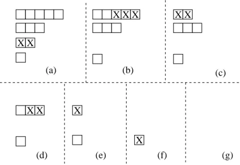
Example: Nim. A position of Nimconsists of several strips, each containing several boxes. A move consists
of removing one or more boxes from a singlestrip. Whoever takes the last box (from the last remaining strip) wins. A sample game of Nimis illustrated in Figure 1.
(a)
X X
X
(g)
(f)
(e)
(d)
X
X
X
X
X
X
(b)
(c)
X
X
Figure 1: The seven sub-figures represent seven consecutive positions in a play of a game of Nim. The last
position is the empty one (with no boxes left and thus no more possible moves). The first six mini-figures also indicate the move taken next (which transforms the current position into the next position): a box marked with ‘X’ is a box that was selected to be taken by the player whose turn it is to play.
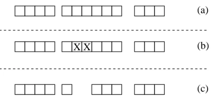
Example: Kayles. A position of Kayles consists of several strips, each containing several boxes, as in Nim. A move consists of removing one or twoadjacent boxes from a single strip. If the player takes a box
(or two) from the middle of a strip then this strip is split into twoseparate strips. In particular, no future move can affect both sides of the original strip. (See Figure 2 for an illustration of one such move.)
Whoever takes the last box (from the last remaining strip) wins.
Example: Dawson’s Kayles. This game is identical toKaylesup to two differences: (1) A move consists
of removingexactly twoadjacent boxes from a single strip. (2) The winning condition is flipped: Whoever makes the last moveloses.
(a)
(b)
X X
(c)
Figure 2: (a) The position before the move – consists of three strips. (b) The move – the selected boxes are marked with ‘X’. (c) The new position – the middle strip was split, leaving four strips.
Winning Conditions and the Difficulty of a Game
All three examples above share some common properties. They are:
Finite. For any given first position, there are only finitely many possible positions that the game may take (throughout its execution).
Loopfree. No position can occur twice in an execution of a game. Once we leave a position, this position will never repeat itself.
Impartial. Both players have the same moves available at all times.
All of the games we will consider in this course have these three properties. As we will further discuss below, the first two properties (finite and loopfree) imply that one of the players must have a perfect winning strategy—that is, a strategy that guarantees a win no matter what his opponent does.
Main Goal: Given a combinatorial game Γ, find an efficient winning strategy for Γ.2
We will consider in this course two possible winning conditions for our games: Normal Play: Whoever makes the last move wins.
Mis`ere Play: Whoever makes the last move loses.
The different winning conditions of the aforementioned games turn out to have a great effect on their difficulty. Nimwas solved in 1902 and Kayleswas solved in 1956. By contrast, the solution toDawson’s Kaylesremains an open problem after 70 years. (That is, we still do not know an efficient winning strategy
for it.)
What makesDawson’s Kaylesso much harder? It is exactly the fact that the last player to move loses.
In general, games with mis`ere play tend to be vastly more difficult. The themes for this course are: 1. Why is mis`ere play more difficult?
2. How can we tackle this difficulty?
2More precisely, we seek a winning strategy that can be computed in polynomial time (measured against the size of asuccinct
description of a game position). In general, any use of the word “efficient” in this course can be safely interpreted to mean “polynomial-time,” though we will be intentionally vague about issues of complexity.
Game Representations and Outcomes
We have mentioned that our goal is to obtain efficient winning strategies for impartial combinatorial games. We will in fact be even more concerned with the structure of individual positions. Therefore, by a “game”
G, we will usually mean an individual position in a combinatorial game.
Sometimes we will shamelessly abuse terminology and use the term “game” to refer to a system of rules. It will (hopefully) always be clear from the context which meaning is intended. To help minimize confusion, we will always denote individual positions by roman letters (G,H,. . .) and systems of rules by Γ.
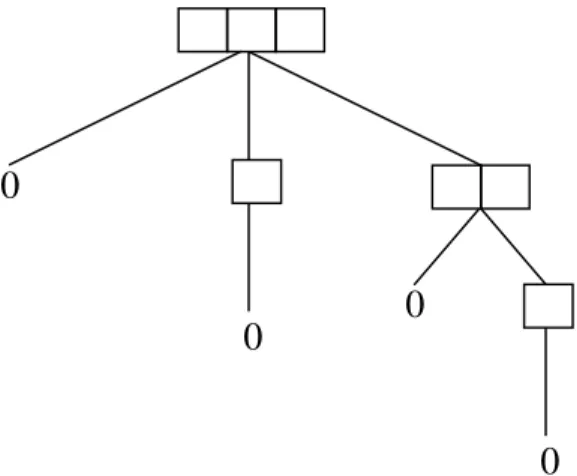
One way to formally represent a game is as a tree. For example, theNimpositionGwhich contains three
boxes in a single strip can be represented by the tree given in Figure 3.
0
0
0
0
Figure 3: Tree representation of theNimpositionGwhich contains three boxes in a single strip
Definition 1.1. Two gamesGandH are identical (isomorphic) if they have isomorphic trees. IfGandH
are identical, we writeG∼=H.
We can also think of theNimpositionGfrom Figure 3 as aset: ={0,,}, where 0 denotes the game{}with no possible moves. We call the positions we can move to directly from a game Gtheoptions ofG. So we are identifyingGwith the set of its options.
We will now introduce some notation that will make it easier to discuss the value of any given position of a game and in particular, the values of Nimpositions.
Definition 1.2. For everyn≥0we denote by∗na strip in Nimof lengthn. We write0and∗as shorthand
for ∗0 and∗1, respectively. Formally, we have
∗n={0,∗,∗2,∗3, . . . ,∗(n−1)}.
As we mentioned above, every game with the properties we have specified has a well-defined outcome (indicating who will win when both players play perfectly). Assuming both players play perfectly, either:
1. The first player has a winning move, or
2. Any move the first player may make will move to a position where he loses. In this case the second player can win.
Definition 1.3. Let Gbe a game. The normal outcomeo+(G)is defined by
• o+(G) =P if second player can winG, assuming normal play;
Likewise, the mis`ere outcome o−
(G)is defined by • o−
(G) =P if second player can winG, assuming mis`ere play;
• o−(G) =N if first player can winG, assuming mis`ere play.
We sayG is a normalP-positionif o+(G) =P, etc.
Note that o+ ando−
have simple recursive descriptions:
o+(G) =P ⇐⇒ o+(G′
) =N for every optionG′ ofG.
o−
(G) =P ⇐⇒ G6= 0 ando−(G′) =N for every optionG′ ofG. P andN are short for previous player andnext player, respectively.
For example, we can consider Nim played with a single strip and see which positions are P-positions
and which areN -positions:
• o+(0) =P: If there are no more boxes, then the previous move was the winning move (the previous
player took the last box).
• o+(∗n) = N for every n > 0: When there is only one strip left, the next player can take all the
remaining boxes and thus win. What about the mis`ere outcomes? • o−
(0) =N : If there are no more boxes, then the previous player took the last box and lost. So the
next player is the winning one. • o−
(∗) =P: When there is only one box left, the next player must take it and lose, so the previous
player is the winning one. • o−(∗
n) =N for everyn >1: Here the winning move is to take all boxes but one.
We now revise our main goal.
Main Goal (Revised): Given a position Gin a combinatorial game, find an efficient way to compute the outcome of G.
In all the examples we consider in this course, the two goals are equivalent: efficient methods for com-puting the outcomes of positions will instantly yield efficient winning strategies.
Disjunctive Sums
The positions in each of our examples naturally decompose. InNim, no single move may affect more than
one strip, so each strip is effectively independent. Both Kaylesand Dawson’s Kayles exhibit an even
stronger form of decomposition: a typical move cuts a strip into two components, and since the components are no longer adjacent, no subsequent move can affect them both.
These observations motivate the following definition.
Definition 1.4. Let Gand H be games. The (disjunctive) sumof Gand H, denoted G+H, is the game played as follows. Place copies ofGandH side-by-side. A move consists of choosing exactly one component and making a move in that component.
Formally, we can defineG+H as the direct sum of the trees forGandH. Or, thinking in terms of sets,
G+H ={G′
+H :G′
is an option ofG} ∪ {G+H′
:H′
is an option ofH}.
In combinatorial game theory, it is customary to be lazy in our use of notation and write simply
G+H ={G′
+H, G+H′
The Strategy for Nim
Here is the strategy for Nim, assuming normal play: write the size of each strip in binary, and then do a
bitwise XOR.Gis aP-position if and only if the result is identically 0. For example, the starting position
of Figure 1(a) has strips of sizes 5, 3, 2 and 1, so we can write 101 = 5 ⊕ 11 = 3 ⊕ 10 = 2 ⊕ 1 = 1
101
The result is nonzero, so Figure 1(a) is anN -position (in normal play).
We will shortly prove a stronger statement that implies this strategy.
Equivalence
We would like to regard two games as equivalent if they behave the same way in any disjunctive sum. For now assume normal play.
Definition 1.5. We say GandH are equal, and write G=H, iff
o+(G+X) =o+(H+X)for every combinatorial gameX.
Note that if G∼=H, then necessarilyG=H, but we will see that nonisomorphic games can be equal. Example. G+ 0 =Gfor any gameG.
Proof. Adding 0 does not change the structure ofGat all. (In fact,G+ 0∼=G.)
Example. G+G= 0 for any gameG.
Proof. We need to show thatX andG+G+X have the same outcome, for anyX.
First suppose o+(X) = P. Second player can win G+G+X as follows. Whenever first player moves
on X, just use the winning strategy there. If first player ever moves on one of the copies of G, make the identical move on the other copy. Second player will get the last move on X because she is following the winning strategy there, and she will get the last move onG+Gby symmetry.
Conversely, ifo+(X) =N, then onG+G+X, just make a winning move onXand proceed as before.
Example. Here is a simple example to show how disjunctive sums can be useful for studying combinatorial games. Consider a Nimposition with strips of sizes 19, 23, 16, 45, 23 and 19. By the previous argument,
the two strips of size 19 together equal 0, as do the two strips of size 23. So this is equivalent toNimwith
strips of sizes 16 and 45.
Exactly the same argument works forKaylesorDawson’s Kayles.
Proposition 1.6.
(a) =is an equivalence relation. (b) IfG=H, thenG+K=H+K.
Proof. (a) is immediate, since equality of outcomes is an equivalence relation. For (b), ifG=H then
o+(G+X) =o+(H+X) for allX,
so in particular
o+(G+ (K+X)) =o+(H+ (K+X)) for allX.
Proposition 1.7. The following are equivalent, for games G, H: (i) G=H
(ii) o+(G+H) =P
Proof. (i)⇒(ii): IfG=H, thenG+G=G+H. ButG+G= 0, soo+(G+H) =o+(0) =P.
(ii) ⇒ (i): By a symmetry argument (just like a previous example), X and G+H +X have the same outcome, for allX. ThereforeG+H = 0, soG+H+H =H. But H+H = 0.
The Sprague–Grundy Theorem
Theorem 1.8 (Sprague–Grundy). For any gameG, there is somem such thatG=∗m. We will in fact prove the following stronger statement.
Definition 1.9. Let S be a finite set of non-negative integers. We define the minimal excludant of S, denoted mex(S), to be the least integer not inS.
Theorem 1.10(Mex Rule). SupposeG∼={∗a1, . . . ,∗ak}. ThenG=∗m, where
m= mex{a1, . . . , ak}.
Proof. By a previous proposition, it suffices to show thatG+∗mis a P-position. There are two cases.
Case 1: First player moves in G. This leaves the position ∗a+∗m, where ∗a is some option of G. Since
m6∈ {a1, . . . , ak}, we necessarily havea6=m. If a > m, second player can move to∗m+∗m; ifa < m, she can move to∗a+∗a. In either case, she leaves aP-position.
Case 2: First player moves in∗m. This leavesG+∗a, for somea < m. Sincemis theminimal excludant of {a1, . . . , ak}, we must havea=aifor somei. Therefore second player can move to∗a+∗a, aP-position.
The Sprague–Grundy theorem follows from one more ingredient.
Exercise. Prove the replacement lemma: suppose G = {G1, . . . , Gk} and suppose G1 =H for some H.
Then
G={H, G2, . . . , Gk}.
Proof of Sprague–Grundy Theorem. WriteG={G1, . . . , Gk}. Inductively, we may assume that G1 =∗a1,
Mis`ere Games and Mis`ere Quotients November 27, 2006
Lecture 2: Octal Games and Mis`ere Play
Instructor: Aaron Siegel Scribes: Omer Kadmiel & Shai Lubliner
We introduce a broad class of games known asoctal games, and then give the definition of mis`ere quotient.
Grundy Value
In the previous lecture we showed:
• Assuming normal play, if G is any game, then G = ∗m for some m. If G = {∗a1, . . . ,∗ak} then
m= mex{a1, . . . , ak}.
• For anyG, H, o+(G+H) =P if and only ifG=H.
We denote byG(G) the unique integermsuch thatG=∗min normal play. G(G) is called the Grundy
value ofG.
XOR and a Winning Strategy for (Normal-Play) Nim
Ifm, nintegers thenm⊕ndenotes the binary XOR of mandn. Theorem 2.1. Let a, b, cbe integers.
o+(∗a+∗b+∗c) =P⇐⇒a⊕b⊕c= 0.
“Proof by Example”. Consider the following example:
11101001 a
⊕ 01101111 b
⊕ 00000111 c
10000001
As the XOR of these values6= 0, we must show that this is anN-position. The first player simply finds
the most significant bit marked 1 in the XOR and chooses any component in which this bit is a 1. In this example, that component is a. He then makes an appropriate move in athat switches the most significant bit to 0, and sets all lower-order bits as needed to make the sum equal 0. Here the winning move is froma
toa′
= 01101000, changing just the first and last bits. a′
⊕b⊕c= 0, so by induction it is aP-position.
Corollary 2.2. ∗a+∗b=∗(a⊕b)
Proof. a⊕b⊕(a⊕b) = 0, so∗a+∗b+∗(a⊕b) = 0.
Example: Dawson’s Kayles
Recall that in Dawson’s Kayles, a move consists of removing exactly two adjacent boxes. We defined Dawson’s Kaylesas a mis`ere-play game, but we can just as easily consider it in normal play. Denote by
Hn a single strip of Lengthn. Then the moves fromHn are to Ha+Hn−2−a, where 1≤a≤n−2.
We can use the Sprague–Grundy theorem and the Nim addition rule to compute normal-play values
H0={}= 0 H1={}= 0 H2={H0}={0}=∗ H3={H1}={0}=∗ H4={H1+H1, H2+H0}={0 + 0,∗+ 0}={0,∗}=∗2 H5={H2+H1, H3+H0}={∗+ 0,∗+ 0}={∗,∗}= 0 H6={H2+H2, H3+H1, H4+H0}={∗+∗,∗+ 0,∗2 + 0}={0,∗,∗2}=∗3
This rapidly becomes tedious, and it’s easily implemented on a computer. The results of a computer calculation are shown in Figure 4. Each row represents a block of 34 Grundy values: the first row shows
G(H0) throughG(H33); the next row showsG(H34) throughG(H67); etc. The number 34 was obviously not
chosen by accident; after a few initial anomalies, a strong regularity quickly emerges with period 34. We now prove a theorem that shows, for a wide class of games, that if such periodicity is observed for “sufficiently long” (in a sense to be made precise) then it must continue forever.
0 0 0 0 0 0 0 0 0 010 0 0 0 0 0 0 0 02 0 0 0 0 0 0 0 0 03 0 1 2 3 4 5 6 7 8 9 0 1 2 3 4 5 6 7 8 9 0 1 2 3 4 5 6 7 8 9 0 1 2 3 0+ 0 0 1 1 2 0 3 1 1 0 3 3 2 2 4 0 5 2 2 3 3 0 1 1 3 0 2 1 1 0 4 5 2 7 34+ 4 0 1 1 2 0 3 1 1 0 3 3 2 2 4 4 5 5 2 3 3 0 1 1 3 0 2 1 1 0 4 5 3 7 68+ 4 8 1 1 2 0 3 1 1 0 3 3 2 2 4 4 5 5 9 3 3 0 1 1 3 0 2 1 1 0 4 5 3 7 102+ 4 8 1 1 2 0 3 1 1 0 3 3 2 2 4 4 5 5 9 3 3 0 1 1 3 0 2 1 1 0 4 5 3 7 136+ 4 8 1 1 2 0 3 1 1 0 3 3 2 2 4 4 5 5 9 3 3 0 1 1 3 0 2 1 1 0 4 5 3 7 170+ 4 8 1 1 2 0 3 1 1 0 3 3 2 2 4 4 5 5 9 3 3 0 1 1 3 0 2 1 1 0 4 5 3 7
Figure 4: Grundy values of Dawson’s Kaylesin normal play.
Octal Games and Octal Codes
Definition 2.3. An octal code is a sequence of digits0.d1d2d3. . . where0≤di<8 for alli.
An octal code specifies the rules for a particular octal game. An octal game is played with strips of boxes, and the code describes how many boxes may be removed and under what circumstances. The digitdk specifies the conditions under whichkboxes may be removed.
Let us consider the bit representation of eachdk: Denotedk =ǫ0+ǫ1·2 +ǫ2·4, where eachǫi= 0 or 1. • We can remove an entire strip of lengthkiffǫ0= 1.
• We can removekboxes from theend of a strip (leaving at least one box) iffǫ1= 1.
• We can removekboxes from themiddle of a strip (leaving at least one box on each end) iffǫ2= 1.
Therefore:
• Dawson’s Kayles is represented by 0.07 as you have to remove exactly two blocks every time from
anywhere in the strip, and you can remove an entire strip of length 2.
• Kaylesis represented by 0.77 as you can remove one or two boxes from a single strip.
• Nim is represented by the infinite sequence 0.3333333. . . as you are allowed to take any number of
boxes from the end or to take an entire strip of any length (but you are not allowed to separate the original strip into two strips).
Guy–Smith Periodicity Theorem
Theorem 2.4(Guy–Smith Periodicity Theorem). Consider an octal game with finitely manynon-zero code digits, and letkbe largest withdk6= 0. Denote byHn a strip of lengthn. Suppose that for somen0>0and
p >0 we have
G(Hn+p) =G(Hn)for everyn withn0≤n <2n0+p+k.
Then
G(Hn+p) =G(Hn)for alln≥n0.
Proof. Note that a move fromHn is always toHa+Hb, wheren−k≤a+b < n. (In taking a whole strip, or from the end of the strip, we may take one or both ofa, bto be 0.)
Now proceed by induction on n. The base case n < 2n0+p+k is given by hypothesis, so assume
n≥2n0+p+k. A move fromHn+p is toHa+Hb wherea+b≥n+p−k.
Sincen≥2n0+p+k, we haven+p−k≥2n0+ 2p, so without loss of generalityb≥n0+p. (Since the
suma+b is greater than or equal to 2(n0+p), at least one of the elements must be at leastn0+p.) By
inductionG(Hb−p) =G(Hb), so
G(Ha+Hb−p) =G(Ha)⊕G(Hb−p) =G(Ha)⊕G(Hb) =G(Ha+Hb).
Here is the picture:
× Hn →Ha+Hb−p
× Hn+p→Ha+Hb
| {z } | {z }
a b
Now Ha +Hb−p is an option of Hn, so we conclude that the options of Hn+p have exactly the same
G-values as those ofHn. Since theG-values ofHn+p andHn both observe the mex rule, we have
G(Hn+p) =G(Hn).
Whenpand n0are as small as possible, we say that Γ has (normal-play)period pandpreperiod n0.
Examples. In normal play: • Kayles(0.77) has period 12.
• Dawson’s Kayles(0.07) has period 34.
• 0.106 has period 328226140474. (See [4].) • 0.007 is not known to be periodic.
Open Problem. Does there exist a finite octal code (i.e., an octal code with finitely many non-zero digits) that yields an aperiodic game?
Mis`
ere Nim
We now considerNim in mis`ere play. It is not hard to show the following. If Gconsists of heaps of sizes
a1, . . . , ak, then
o−(G) =P ⇐⇒a1⊕a2⊕ · · · ⊕ak= 0,
unless everyai is equal to 0 or 1. In that case,o−(G) =P ⇐⇒a1⊕ · · · ⊕ak= 1.
So the strategy for mis`ere Nimis: play exactly like in normalNim, unless your move would leave only
Mis`
ere Equality
We now make the exact same definition of equality as before (cf. Definition 1.5), this time assuming mis`ere play.
Definition 2.5.
G=H⇐⇒o−(G+X) =o−(H +X)for allX
Recall that in normal play any two P-positions are equal (and in particular, anyP-position is equal to
0). We shall see that this is not the case in mis`ere play. In mis`ere play:
• 0 is an N-position.
• ∗ is aP-position.
• ∗2 is anN -position.
This we have already seen. Note that∗2 +∗2 is also aP-position. No matter what first player does, second
player can always respond by moving to∗: ∗2 +∗2 % % K K K K K K K K K K * * U U U U U U U U U U U U U U U U U U ∗2 + 0 y y ssss ssss ss ∗2 +∗ t t iiiiii iiiiii iiiiii i ∗+ 0
This immediately shows that∗2 +∗26= 0, since∗2 +∗2 is aP-position but 0 is anN -position. In fact, we
will now show that∗2 +∗26=∗, thus exhibiting two distinct P-positions.
Proposition 2.6. ∗+∗= 0.
Proof. Whoever can winX can also winX+∗+∗: he follows the winning strategy onX, and if his opponent ever moves on one copy of∗, he responds by moving on the other. This guarantees that his opponent will make the last move onX, leaving either 0 or∗+∗. But both of these areN -positions.
Now∗+∗2 +∗2 is anN -position, since it has a move to ∗2 +∗2. The following proposition therefore
shows that∗ 6=∗2 +∗2.
Proposition 2.7. ∗2 +∗2 +∗2 +∗2 is aP-position.
Proof. The options are∗2 +∗2 +∗2 + 0 and∗2 +∗2 +∗2 +∗. But these have moves to∗2 +∗2 + 0 + 0 and ∗2+∗2+∗+∗, respectively. By the previous proposition, both of these are equal to∗2+∗2, aP-position.
In fact, it is possible to show that∗2 +∗26=∗mfor anym. So even among sums ofNim-heaps, we have
games that are not equivalent to anyNim-heap. This contrasts sharply with the situation in normal play,
whereevery game is equivalent to aNim-heap.
We have seen that ∗+∗= 0. There are very few other identities we can establish in mis`ere play. Here are really the only two:
Exercise (Mis`ere Mex Rule). SupposeG∼={∗a1, . . . ,∗ak}. ThenG=∗m, where
m= mex{a1, . . . , ak},
Exercise. For anym, we have ∗m+∗=∗(m⊕1). (cf. Corollary 2.2) The mis`ere mex rule is spectacularly false if everyai≥2. For example, let
G={∗2},
the game whose only option is ∗2. (G is sometimes called∗2#.) Gis aP-position, so right away we have
G6= 0. As an exercise, show that G is not equal to any∗m. In fact, it is possible to show that G is not equal to anysum of Nim-heaps, but we won’t do that in this course.
Birthdays
Clearly, things are more complicated in mis`ere play than in normal play. We now state a result that shows just how much worse they are.
Definition 2.8. The birthdayof a game Gis the height of its game tree.
Innormal play there are just six games with birthday≤5: 0,∗,∗2,∗3,∗4, and∗5. In mis`ere play, there are 4171780. On day 6 there are more than 24171779. . .
The theory of mis`ere games modulo = is beautiful and fascinating, but these results suggest that it is not terribly useful: we very quickly run into seemingly intractable complications. We will not say much more about this “global theory” in this course; the interested reader is referred to [2].
Mis`
ere Quotients
IfG=H, then G+X and H+X have the same outcomes, for any gameX. As we’ve just observed, this equality relation gives rise to a virtually intractable theory. The problem is that G = H is too strong a relation—we are requiring thatGandH behave identically in any context, which is asking a bit too much.
Key Idea: Suppose we just want to know how to playKayles(for example). We just need to
specify how a KaylespositionGinteracts with other positions that actually occur inKayles.
With this in mind, fix a setA of games (usually,A will be the set of positions that occur in some octal
game). Assume thatA is closed under addition.
Definition 2.9. Let A be a set of games, closed under addition. Then forG, H∈A,
G≡A H ⇐⇒o−(G+X) =o−(H+X)for allX ∈A.
Compare this to Definition 2.5: we are restricting the domain of games that can be used to distinguish
Gfrom H. This coarsens the equivalence and allows us to recover a tractable theory. Very often, the set of equivalence classes modulo ≡A is finite, even when A is infinite. (It is trivial to see that ≡A is an
equivalence relation, since outcome-equality is an equivalence relation.) Now, think of normal-play Grundy values as elements of the group
D=M
N
Z2,
a (countably) infinite direct sum of copies of Z2 (one for each binary digit). The Sprague–Grundy theory
maps each game G to an element of D, thus representing the normal-play structure of G in terms of the group structure of D. We will show that the equivalence classes modulo≡A function as a localized mis`ere analogue of the Sprague–Grundy theory.
We will make a slightly stronger assumption onA than closure under addition.
Definition 2.10. A set of games A is hereditarily closedif, for any G∈A and any option G′ of G, we
Definition 2.11. A is closed if it is both hereditarily closed and closed under addition.
Note that ifA is the set of positions that occur in an octal game, thenA is closed. In fact, virtually all
sets of games that are interesting to us are closed, so there is little harm in making this assumption. Example. LetA ={all sums of ∗and∗2}, that is,
A ={m· ∗+n· ∗2 :m, n∈N}.
Let’s compute the equivalence classes modulo≡A.
• ∗ 6≡A 0, since∗ is aP-position and 0 is anN -position.
• Likewise,∗26≡A ∗since∗2 is anN -position. Further,∗26≡A 0: letX =∗2; then∗2 +X=∗2 +∗2 is
a P-position, but 0 +X =∗2 is an N-position.
• Finally,∗2 +∗ 6≡A ∗ since it’s anN -position;∗2 +∗ 6≡A 0, since they’re distinguished byX =∗; and
∗2 +∗ 6≡A ∗2, since they’re distinguished byX =∗2. This gives four equivalence classes:
[0] [∗] [∗2] [∗2 +∗]
N P N N
Are there others?
• Yes! ∗2 +∗2 is aP-position, so it’s either equivalent to∗, or a new equivalence class. But:
– ∗+ (∗2 +∗2) is anN-position, since it has a move to∗2 +∗2, which isP;
– ∗2 +∗2 + (∗2 +∗2) is aP-position (Proposition 2.7).
Therefore∗ 6≡A ∗2 +∗2.
• Similar reasoning shows that ∗2 +∗2 +∗ gives yet another equivalence class. So we have six equivalence classes total:
[0] [∗] [∗2] [∗2 +∗] [∗2 +∗2] [∗2 +∗2 +∗]
N P N N P N
We now show that these are the only six.
Lemma 2.12. Let n≥1. Thenn· ∗2is aP-position iffn is even.
Proof. Ifnis even, then second player’s strategy is to cancel out copies of∗2 (using the fact that∗+∗= 0) until we get down to∗2 +∗2, which is known to be aP-position.
Ifnis odd,n≥3, then first player can win by moving to (n−1)· ∗2. Finally, ifn= 1, then first player simply moves to∗.
Lemma 2.13. Let n≥1. Thenn· ∗2 +∗ is always anN -position.
Proof. Ifnis even, then the winning move is ton· ∗2, which is aP-position by the previous Lemma.
Ifnis odd, n≥3, then the winning move is to (n−1)· ∗2 +∗+∗, which again is aP-position, since
∗+∗= 0.
Finally, if n= 1, then the winning move is to 0 +∗. Corollary 2.14. SupposeG=m· ∗+n· ∗2 andX=m′· ∗
+n′· ∗2. If
n≥1, then the outcome ofG+X
Proof. Follows immediately from the previous two Lemmas and the fact that∗+∗= 0. Corollary 2.15. LetG=m· ∗+n· ∗2 andH =m′· ∗
+n′· ∗2.
Ifn, n′≥1, m≡m′ (mod2), andn≡n′ (mod2), thenG≡A H.
Corollary 2.16. There are exactly six equivalence classes modulo≡A.
Proof. By the previous corollary, everyG∈A is equivalent to m· ∗+n· ∗2, for some m <2 and n <3.
There are only six such possibilities, and we’ve already shown that all six are mutually inequivalent. Warning. We’ve just shown that∗2 +∗2 +∗2≡A ∗2. However, equality doesnot hold:
Exercise. Show that∗2 +∗2 +∗26=∗2. (Hint: tryX =∗2#1, defined by ∗2#1 ={∗2#,∗}={{∗2},∗}.)
This shows that the equivalence≡A is a genuine coarsening of equality. There exist unequal games that are equivalent moduloA.
This finishes our example. We now return to the general context.
Lemma 2.17. Let A be any closed set of games andG, H∈A. IfG≡A H andK∈A, thenG+K≡A
H+K.
Proof. ForX∈A, we have
o−
((G+K) +X) =o−
(G+ (K+X)) ando−
(H+ (K+X)) =o−
((H+K) +X).
But A is closed, so K+X ∈ A. Since G ≡A H, we have o−(G+ (K+X)) = o−(H + (K+X)), as
needed.
Moreover, sinceA is hereditarily closed, we have 0∈A. So the equivalence class of 0 is an identity, and
in fact we have a monoid.
Definition 2.18. Asemigroupis a set S equipped with an associative binary operation ·. That is, • If x, y∈S, then x·y∈S;
• If x, y, z∈S, thenx·(y·z) = (x·y)·z.
A semigroupS is a monoidif it has an identity, and commutativeif its operation is commutative. We’ve shown that the equivalence classes ofA modulo≡A form a commutative monoidQ.
Q={[G]≡A :G∈A}.
Furthermore, ifG≡A H, then sinceo−
(G+ 0) =o−
(H+ 0), we have
Gis aP-position⇐⇒H is a P-position.
So we can define a subsetP ⊂ Qby
P={[G]≡A :G∈A is aP-position}.
Example. Let’s sketch the structure ofQ(A) for our example A ={sums of ∗ and ∗2}.
Denote by Φ :A → Qthe quotient map
Φ(G) = [G]≡A.
NowA is generated (as a monoid) by∗and∗2. Put
1 = Φ(0) = [0] a= Φ(∗) = [∗] b= Φ(∗2) = [∗2].
We know that∗+∗= 0, so in facta2 = 1. Furthermore, we’ve seen that∗2 +∗2 +∗2 ≡A ∗2, so we have
b3=b. But we also know that the six elements
A [0] [∗] [∗2] [∗2 +∗] [∗2 +∗2] [∗2 +∗2 +∗]
↓
Q 1 a b ab b2 ab2
are all distinct. ThusQ={1, a, b, ab, b2, ab2} and we have the presentation
Q ∼=ha, b|a2= 1, b3=bi.
Since ∗ and ∗2 +∗2 are the only P-positions (up to equivalence), we also have P = {a, b2}. This mis`ere
Mis`ere Games and Mis`ere Quotients November 28, 2006
Lecture 3: The Periodicity Theorem
Instructor: Aaron Siegel Scribes: Amir Kantor & Gideon Amir
Definition 3.1 (Definitions). Let A be any set of games. Define
hcl(A),{subpositions of all games in A},
cl(A),Closure under addition of hcl(A).
Remark. cl(A) is hereditarily closed. To see this, let G = G1+G2+. . .+Gk where Gi ∈ hcl(A).
W.l.o.g.G′
=G′
1+G2+. . .+Gk. We know thatG′1∈hcl(A) since the latter is hereditarily closed.
Example. cl({∗2}) ={sums of∗,∗2}={i· ∗+j· ∗2 :i, j∈N}. Exercise.
• If A ⊆B andBis closed, then cl(A)⊆B.
• cl(cl(A)) = cl(A).
Definition 3.2. If A is not closed,Q(A),Q(cl(A)). We sometimes write Q(G),Q(cl ({G})). Example. T2∼=Q(∗2).
Quotients of Octal Games
Let’s consider the context of a specific octal game, such asKayles. Denote byHn aKaylesheap of sizen
and letA be the set of allKaylespositions; that is,
A = cl(H0, H1, H2, H3, . . .).
Let (Q,P) be the mis`ere quotient forKaylesand consider the quotient map Φ :A → Q.
Remark. If we know Φ(Hn) for all n, then if G = Hn1 +· · ·+Hnk we can easily compute Φ(G) =
Φ(Hn1)· · ·Φ(Hnk). So, in order to specify Φ, it suffices to specify the single-heap values Φ(Hn).
Themain point is:
Suppose we knowQ(A), together with Φ(Hn) for alln. If we want to knowo−
(G) forG∈A, we
can writeG=Hn1+· · ·+Hnk, compute Φ(G) = Φ(Hn1)· · ·Φ(Hnk), and simply look up whether
Φ(G)∈ P. If the quotient is finite, we’ve reduced the problem of findingo−
(G) to a small number of operations on a finite multiplication table. This yields an efficient way to compute o−
(G).
So we direct our energies at computing the values of Φ(Hn) for alln. In practice, we can construct good algorithms for computing quotients of a finite number of heaps. (We won’t have time to discuss them in this course; see [13, Appendix A].) If we run these algorithms onKaylesto heap 120, we get the result shown
in Figure 5.
Now examine the Φ-values Φ(Hn)∈ Q. We observe that
Φ(Hn+12) = Φ(Hn), for 716n6120−12.
This situation is much like the periodicity ofG-values that we observed in normal play.
The following notation will be very useful; it applies toKaylesas well as to an arbitrary octal game Γ.
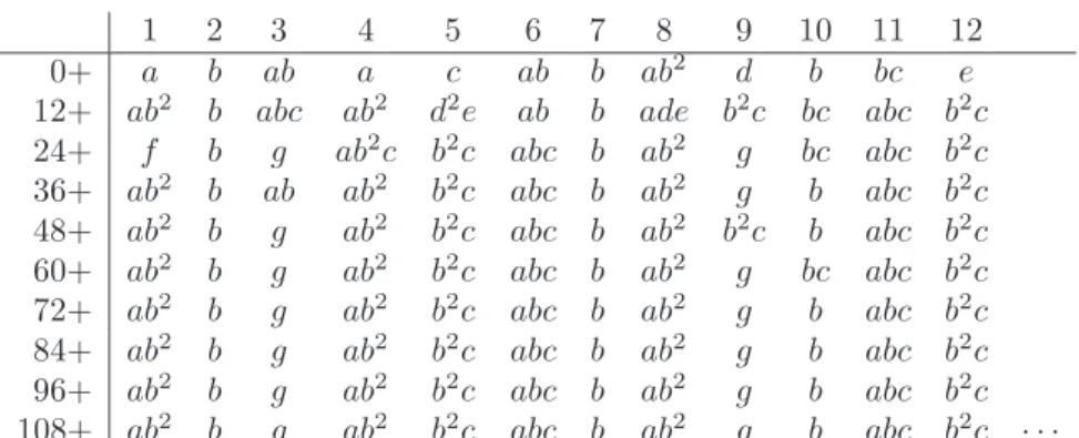
Q(H0, H1, H2, . . . , H120)∼=ha, b, c, d, e, f, g |a2= 1, b3=b, bc2=b, c3=c, bd=bc,
cd=b2, d3=d, be=bc, ce=b2, e2=de,
bf=ab, cf =ab2c, d2f =f , f2=b2, b2g=g,
c2g=g, dg=cg, eg=cg, f g=ag, g2=b2i
P ={a, b2, ac, ac2, d, ad2, e, ade, adf}
1 2 3 4 5 6 7 8 9 10 11 12
0+ a b ab a c ab b ab2 d b bc e
12+ ab2 b abc ab2 d2e ab b ade b2c bc abc b2c
24+ f b g ab2c b2c abc b ab2 g bc abc b2c 36+ ab2 b ab ab2 b2c abc b ab2 g b abc b2c 48+ ab2 b g ab2 b2c abc b ab2 b2c b abc b2c 60+ ab2 b g ab2 b2c abc b ab2 g bc abc b2c 72+ ab2 b g ab2 b2c abc b ab2 g b abc b2c 84+ ab2 b g ab2 b2c abc b ab2 g b abc b2c 96+ ab2 b g ab2 b2c abc b ab2 g b abc b2c 108+ ab2 b g ab2 b2c abc b ab2 g b abc b2c · · ·
Figure 5: Quotient presentation and pretending function for mis`ereKaylesto heap 120.
• A the set of all positions,A = cl(H0, H1, . . .).
• Q(Γ) =Q(A).
• An the set of all positions with no heap larger than n,An= cl(H0, . . . , Hn).
• Qn(Γ) =Q(An), the nth partial quotient for Γ.
We’ve computed Q120(Kayles), and the quotient map Φ120:A120−→ Q120, and found that it is periodic
past a certain point.
A Brief Digression
In a moment we will state a mis`ere version of the periodicity theorem. We first pause to consider some potential difficulties.
Remark. Suppose we computed Qn. Now we throw Hn+1 into the quotient. There might be games
G, K∈Ansuch thatG≡AnKbut are distinguished byHn+1. When this happens, we have Φn(G) = Φn(K),
but Φn+1(G)6= Φn+1(K).
This remark shows that we must be careful not to confuse the partial quotients of Γ with its full quotient. Note that in normal play, there is no such concern. Given a set of gamesA, it is possible to definenormal
equivalence modulo A in exactly the same way we’ve defined mis`ere equivalence modulo A. However, in
normal play it will always be the case thatG≡A Kif and only if G=K. That is, in normal play, local and global equivalence coincide. (To see this, observe that if G6=K in normal play, then Gand K must have different Grundy values, soG+GandG+K have different outcomes. So ifGandK are distinguished by anything, then they must be distinguished locally, byGitself.) So, although the sorts of localizations we’re discussing are perfectly applicable to normal play, they don’t provide any further resolution (and in a sense, they don’t need to, because normal play is simple enough to begin with).
Let us consider another difference between normal play and mis`ere play. Consider a finitely generated set A. Innormal play, there can be only finitely many G-values represented. To see this, letH1, . . . , Hn
generateA. Then theG-values represented byA are bitwise exclusive-or’s ofG(H1), . . . ,G(Hn), but these
What about mis`ere play? IsQ(A) finite? Answer: Not in general. Later in this course we will see an
example of an infinite, finitely generated quotient. Our picture of such quotients is still very hazy. In fact, the following question is still open.
Open Problem. Specify an algorithm to determine whether Q(A)is infinite, assumingA is finitely
gen-erated.
We’ll say more about this later in the course. Finally, now is as good a time as any to interject the following remark:
Remark. All monoids we consider in this course are commutative. Sometimes I will slip and say “monoid” when I really mean “commutative monoid.”
Periodicity
We now return to the setting of an octal game Γ with heapsHn. Recall: Periodicity theorem for normal play:
Let Γ be an octal game with last non-zero code digit k. Suppose there are integers n0, p such
that G(Hn+p) =G(Hn) forn0≤n <2n0+p+k. Then in fact G(Hn+p) =G(Hn) for alln≥n0.
Theorem 3.3 (Periodicity Theorem for Mis`ere Play). Let Γ be an octal game with last non-zero code digit k. Fix n0, p and letM = 2n0+ 2p+k. Let(QM,PM) =QM(Γ). Suppose that ΦM :AM −→ QM, and that ΦM(Hn+p) = ΦM(Hn) for n0≤n <2n0+p+k. Then in fact
Q(Γ)∼=QM(Γ), and
Φ(Hn+p) = Φ(Hn)for all n≥n0.
Proof. Recall the proof for normal play. By induction onn:
× Hn
× Hn+p
| {z } | {z }
a b
Hn+p −→Ha+Hb is a typical move fromHn+p. We chose the upper bound of our induction base case
to be large enough that one of a, b ≥ n0+p. Assume w.l.o.g that it’s b. But then G(Hb−p) = G(Hb),
so G(Ha+Hb) = G(Ha +Hb−p). We conclude that the options of Hn and Hn+p represent exactly the
sameG-values. ButG-values are computed by the mex rule, so this impliesG(Hn+p) =G(Hn).
To prove the periodicity theorem for mis`ere play, we can use exactly the same argument to show that the options ofHn, Hn+prepresent exactly the same ΦM-values. So the proof now depends only on the following lemma.
Lemma 3.4. SupposeA is a closed set of games, andGis a game all of whose options are inA. Assume
that, for someH ∈A,
{Φ(G′) :G′ is an option of G}={Φ(H′) :H′ is an option ofH}.
Assuming Lemma 3.4, the proof of the periodicity theorem is complete. For we can go by induction to show that
QM(Γ)∼=QM+1(Γ)∼=QM+2(Γ)∼=. . . ,
and that the resulting Φ-values are periodic.
Bipartite Monoids
Although we could prove Lemma 3.4 directly, it will be easier after we introduce a suitable abstraction of the mis`ere quotient construction. Since the abstract setting is also useful in other situations, this is worth the effort.
Definition 3.5. Abipartite monoidis a pair(Q,P)whereQis a commutative monoid, andP ⊂ Qis some subset. We will usually write b.m. for bipartite monoid.
Definition 3.6. Let (Q,P)be a b.m. x, y∈ Q are said to be indistinguishableif, for all z∈ Q,
xz ∈ P ⇐⇒yz∈ P.
Definition 3.7. A b.m. (Q,P)is reducedif the elements ofQare pairwise distinguishable. We write r.b.m. for reduced bipartite monoid.
Example. Every mis`ere quotient is a r.b.m.
Proof. Suppose [G]≡A and [H]≡A are indistinguishable. Then for anyX ∈A,
[G] + [X]∈ P ⇐⇒[H] + [X]∈ P.
Thereforeo−
(G+X) =o−
(H+X) for allX ∈A, so [G] = [H].
Example. If A is a closed set of games, andB is the set of mis`ereP-positions ofA, then (A,B) is a
bipartite monoid. The same is true if we takeBto be the set of normalP-positions ofA.
Definition 3.8. A function f : (Q,P)→ (S,R) is a bipartite monoid homomorphism if f : Q → S is a monoid homomorphism, and for everyx∈ Q, we have x∈ P iff f(x)∈ R.
Definition 3.9. Let (Q,P) and(S,R) be bipartite monoids. (S,R) is a quotient of (Q,P) iff there is a surjective homomorphism f : (Q,P)→(S,R).
Definition 3.10. Let (Q,P)be a b.m. Define a relation ρonQ byxρy iffxandy are indistinguishable. Exercise. Show thatρis an equivalence relation, and that the equivalence classes modulo ρform a bipartite monoid.
Definition 3.11. The reduction of (Q,P) is the bipartite monoid of equivalence classes modulo ρ. We denote it by(Q′,P′).
Exercise. Show that(Q′,P′)is reduced and is a quotient of (Q,P).
Example. Let A be a closed set of games, and let B be the set of mis`ereP-positions in A. Then the
mis`ere quotientQ(A) is the reduction of (A,B).
Proposition 3.12. Suppose(Q,P)is a b.m. with reduction(Q′
,P′
). Let(S,R)be any quotient of(Q,P), viaf : (Q,P)→(S,R), and let(S′
,R′
)be its reduction. Then there is an isomorphismi: (Q′
,P′
)→(S′
,R′
) making the following diagram commute:
Q f / /S Q′ i S′
Proof. Letρbe the reduction relation onQ(Q′
=Q/ρ), and letτ be the reduction relation onS(S′
=S/τ). Now forx, y ∈ Q, we have:
[x]ρ= [y]ρ iff xz∈ P ⇔yz∈ Pfor allz∈ Q iff f(xz)∈ R ⇔f(yz)∈ Rfor allz∈ Q
iff f(x)w∈ R ⇔f(y)w∈ Rfor allw∈ S (sincef is surjective) iff [f(x)]τ = [f(y)]τ
So we may define the mapibyi([x]ρ) = [f(x)]τ. We just showed thati is well-defined and one-to-one. Sincef is surjective, so isi, and it follows thatiis an isomorphism. Commutativity of the diagram follows trivially from the definition ofi.
Corollary 3.13. Every bipartite monoid has exactly one reduced quotient (up to isomorphism).
Let us see why this is important. LetA be a closed set of games, andBthe set of mis`ereP-positions in A. Then the mis`ere quotientQ(A) is the reduction of (A,B). Therefore, suppose we have some putative
quotient (Q,P), and we want to assert that it isQ(A). We just need to show that:
(a) (Q,P) is reduced; and
(b) (Q,P) is a quotient of (A,B).
By Proposition 3.12, these conditions imply that (Q,P) ∼=Q(A). We can therefore avoid the exhaustive
Mis`ere Games and Mis`ere Quotients November 29, 2006
Lecture 4: More Examples
Instructor: Aaron Siegel Scribes: Shai Lubliner & Ohad Manor
Proof of Lemma 3.4
We now prove Lemma 3.4, thus completing the proof of the Periodicity Theorem.
Definition 4.1. SupposeA is a set of games, and Gis a game all of whose options are inA. Define
Φ′′G={Φ(G′) :G′ is an option ofG}.
(This definition includes the case when G∈A.)
Lemma 4.2. SupposeA is a closed set of games and(Q,P)a r.b.m. The following are equivalent:
(i) (Q,P)∼=Q(A);
(ii) There exists a surjective monoidhomomorphism Φ :A → Q, such that for allG∈A,
Φ(G)∈ P ⇐⇒ G6= 0andΦ(G′
)6∈ P for every option G′
of G.
Proof. (i)⇒(ii): Let Φ be the quotient mapA → Q(A). We know that, for allG,
Gis aP-position ⇐⇒ G6= 0 and everyG′ is anN -position.
But since Φ is a homomorphism of bipartite monoids, we have
X is aP-position ⇐⇒ Φ(X)∈ P, for allX ∈A,
and the conclusion follows immediately.
(ii) ⇒(i): By Corollary 3.13, Q(A) is the unique reduced quotient of (A,B) (where Bis the set of P
-positions inA). Thus it suffices to show that Φ is a homomorphism of bipartite monoids, since this implies
that (Q,P) is a quotient of (A,B). So we must prove the following, for allG∈A:
Gis aP-position iff Φ(G)∈ P.
Now by induction onG(i.e., on the height of the game tree ofG), we may assume that
G′
is aP-position iff Φ(G′)∈ P,
for all optionsG′ ofG. But now:
Φ(G)∈ P iff G6= 0 and Φ(G′)6∈ P for allG′ (by assumption)
iff G6= 0 and everyG′ is anN -position (by induction)
iff Gis aP-position (by definition ofP-position).
This proves the lemma.
Proof of Lemma 3.4. Assume A is a closed set of games, all options of G are in A and Φ′′G = Φ′′H for
someH ∈A. We must show thatQ(A ∪ {G})∼=Q(A) and Φ(G) = Φ(H).
• Φ+(G) = Φ(H);
• Φ+(Y) = Φ(Y) for all Y ∈A.
If we regardGas a free generator of the monoid cl(A ∪ {G}) overA, then this defines a monoid
homomor-phism. So we just need to show that Φ+satisfies condition (ii) of Lemma 4.2.
Fix X ∈ cl(A ∪ {G}). We can writeX =n·G+Y for some n ≥0 and Y ∈ A. The case n= 0 is
already known, so we can assumen≥1. LetW =n·H+Y; clearly Φ+(X) = Φ+(W).
Now consider an optionX′
ofX. We haveX′ =n·G+Y′ or (n−1)·G+G′ +Y. • IfX′ =n·G+Y′ , then Φ+(X′ ) = Φ+(n·H+Y′ ), which is an option of W. • If X′ = (n−1)·G+G′ +Y, then Φ+(X′ ) = Φ+((n−1)·H+G′ +Y). But since Φ′′ G= Φ′′ H, there must be some H′ with Φ+(H′ ) = Φ+(G′ ). So Φ+(X′ ) = Φ+((n−1)·H +H′ +Y), again an option ofW′ .
This shows that (Φ+)′′
X ⊂(Φ+)′′
W, and an identical argument shows that (Φ+)′′
W ⊂(Φ+)′′ X. But since W ∈A, we know that Φ(W)∈ P ⇐⇒ W 6= 0 and Φ(W′ )6∈ P for allW′ .
Since Φ+(X) = Φ+(W) and (Φ+)′′X = (Φ+)′′W, we have
Φ+(X)∈ P ⇐⇒ W 6= 0 and Φ+(X′
)6∈ P for allX′
.
This satisfies Lemma 4.2(ii) except for the conditionW 6= 0. But if either ofG, H is identically 0, then both must be, since Φ′′
G=∅ iff Φ′′
H =∅. ThereforeW 6= 0 iffX 6= 0, and we are done.
Further Examples
The partial quotients of Nimare fundamental examples, and we denote them byTn.
• T0=Q(0);
• T1=Q(∗);
• T2=Q(∗2);
• Tn=Q(∗2n−1).
Here are their presentations: • T0={1};P =∅
• T1=ha|a2= 1i;P ={a}
• T2=ha, b|a2= 1, b3=bi;P ={a, b2}
• T3=ha, b, c|a2= 1, b3=b, c3=c, b2=c2i;P ={a, b2}
• Tn=ha, b1, b2, . . . , bn−1 |a2= 1, b3i =bi, b21=b22=· · ·=bn2−1i;P ={a, b21}
To find Φ(∗m) (in any of theTn), write min binary, as· · ·ǫ3ǫ2ǫ1ǫ0, and we have
Φ(∗m) =aǫ0·bǫ11 ·b
ǫ2
2 · · · · ·b
ǫn
n . For example, inT4, we have
Φ(∗4) =b2, Φ(∗5) =ab2, Φ(∗6) =b1b2, Φ(∗7) =ab1b2, Φ(∗8) =b3
Notice that we always have
b2 1=b 2 2=· · ·=b 2 n−1
Denote this element byz. zrepresents the sum∗m+∗m, forany Nim-heap withm≥2. In fact, it represents
The Structure of
T
nLet’s write out the elements ofT3.
T3={1, a, b1, ab1, b2, ab2, b1b2, ab1b2, z, az}
Consider the subset
K={b1, ab1, b2, ab2, b1b2, ab1b2, z, az}
Observe thatz·z=z,z·b1=b1, andz·b2=b2. Thereforez is an identity ofK andx2=zfor allx∈ K.
SoKis a group, and we have
K ∼=Z3 2.
In factK behaves just like normal playG-values: it has eight elements, corresponding one-to-one withNim
positions ofG-value 0 through 7.
Recall the strategy for mis`ereNim: play exactly like in normalNim, unless your move would leave only
heaps of size 0 or 1. In that case, play to leave an odd number of heaps of size 1.
Kcorresponds to the “exactly like normalNim” clause of this strategy: it is isomorphic to the
normal-play quotient of∗4. The two elements 1 andacorrespond to the “unless”: they represent positions with all heaps of size≤1.
Note that everyTn, forn≥2, can be written asK ∪ {1, a}, whereK ∼=Zn
2. K is called thekernel of the
monoid, and in the next lecture we will see how to generalize it. In particular we have:
• |T0|= 1
• |T1|= 2
• |Tn|= 2n+ 2 for alln≥2
We can also define the full quotient of Nim:
T∞=Q(0,∗,∗2,∗3,∗4, . . .)∼=ha, b1, b2| a2= 1, bi3=bi, b21=b 2
2=. . .i P ={a, b 2 1}
Remember that normal-playG-values look like
M N
Z2
Well, we can writeT∞=K∞∪ {1, a}in exactly the same way, and we haveK∞∼=LNZ2.
Tame and Wild Quotients
Definition 4.3. A set A is tame iffQ(A)∼=Tn for somen∈N∪ {∞}. Otherwise it is wild.
Not all quotients are tame:
Example. LetG=Q(∗2#320), where∗2#320 ={0,∗2,∗3,∗2#} and∗2#={∗2}. We have Q(G)∼=ha, b, t |a2= 1, b3=b, t2=b2, bt=bi; P={a, b2}
This quotient is calledR8. It is very common; many octal games have quotientR8, including (for example)
0.75. In fact, it can be shown that R8 is the smallest quotient except forT0, T1, T2. The quotient map is
given by (writingz=b2, as before)
Notice thatR8 is justT2with two extra elements: Q={1, a, b, ab, z, az | {z } K | {z } T2 , t, at} NowK ∼=Z2
2, and{1, a}is a (separate) isomorphic copy ofZ2. But{t, at}is not a group, becauset2=z∈ K.
The right picture ofR8is this: it is the union
K ∪ {1, a} ∪ {t, at},
whereKand{1, a}are two disjoint groups, and{t, at}are two extra elements that are “associated” withK. We’ll say more about this in the next lecture.
General Structure
Lemma 4.4. Suppose that A is hereditarily closed, A 6=∅, andA 6={0}. Then necessarily∗ ∈A.
Proof. ∗is the only game whose only option is 0.
Proposition 4.5. Let (Q,P)be any nontrivial mis`ere quotient. Then for all x∈ Q, there is some y ∈ Q withxy∈ P.
Proof. Write (Q,P) =Q(A) and chooseG∈A with Φ(G) =x. First supposeG= 0. Thenx= 1. By the
assumption of nontriviality, we haveA 6={0}, so by the previous lemma ∗ ∈A. But Φ(∗)∈ P and 16∈ P,
so we can takey= Φ(∗).
Now assumeG6= 0, and considerG+G. If it is aP-position, then we are done, withy=x. Otherwise,
some option ofG+Gmust be aP-position, sayG+G′
. So we can takey= Φ(G′
). Proposition 4.6. For any Gand any option G′
,Φ(G)6= Φ(G′
). Proof. Exercise. (Hint: Use the previous proposition.)
Proposition 4.7. If A is nontrivial andG∈A, thenG6≡A G+∗
Proof. By Proposition 4.5, there is a gameH∈Asuch thatG+H is aP-position. But thenG+H+∗is
anN-position, soH distinguishesGfromG+∗.
Corollary 4.8. Every nontrivial mis`ere quotient has even order. Proof. Exercise. (Hint: Consider the mappingx7→ax.)
In fact, one can prove the following facts.
• T1is the only quotient of order 2. (Immediate from Lemma 4.4)
• There are no quotients of order 4. (Proved in [13]) • T2is the only quotient of order 6. (Also proved in [13])
Mis`ere Games and Mis`ere Quotients November 30, 2006
Lecture 5: Further Topics
Instructor: Aaron Siegel Scribes: Shiri Chechik & Menachem Rosenfeld
In this lecture, we will discuss four interesting problems, most of which have not yet been solved completely. We will also discuss the structure of finite commutative monoids.
Four interesting problems
1. Infinite Quotients
We can think of infinite quotients as belonging to either one of two categories: Those that are finitely generated, and those that are not. We have already seen one infinite quotient, T∞ =Q(0,∗,∗2, . . .). It is
not finitely generated. Every one of its finitely generated submonoids is finite, and it is built up from these finite quotients. It is therefore not an interesting quotient to study.
There also exist finitely generated infinite quotients. We can find an example of this by denoting
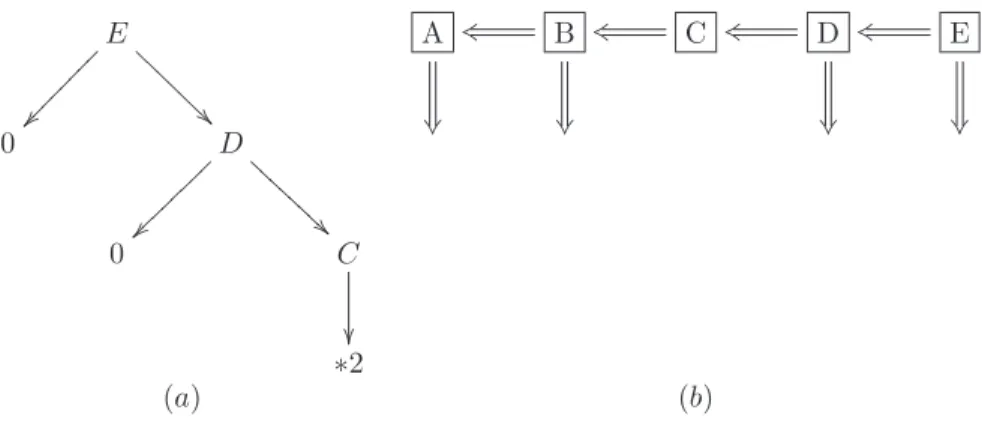
A=∗, B=∗2, C={B}=∗2#, D=∗2#0 ={C,0}, andE={D,0}=∗(2#0)0. Figure 6(a) shows the game tree ofE.
E @ @ @ @ @ @ @ 0 D ~ ~ ~~~~ ~~~~ A A A A A A A A 0 C ∗2 A B k s C k s D k s E k s (a) (b)
Figure 6: Two representations for the gameE=∗(2#0)0. (a) The game tree ofE. (b) A visual representation
of cl(E).
Denoting A = cl(E), a visual way to understand a game in A is suggested in Figure 6(b); for every
game, there are several coins in every box, and a move consists of moving a coin along an arrow (either one step to the left, or from boxes other thanC, outside the game board). The last player to move loses.
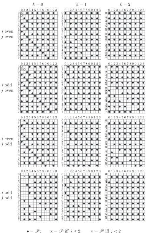
As it turns out,|Q(E)|=∞, but every game with a smaller tree has a finite quotient. So E is in some sense the simplest game that gives rise to an infinite quotient. To understand why the quotient is infinite, first note that every X ∈ A can be written as X = iA+jB +kC+lD+mE. In [13, Section 6], we
compute the outcome of every such X. It turns out that when k ≥3, the outcomes follow a simple rule:
o−
(X) =P ⇐⇒ i+l andj+mare both even. However, whenk≤2, the outcomes can be quite erratic.
See Figure 7. Each table represents the outcomes for a particular choice of (i, j, k). Within each table, there is a dot at (rowm, columnl) iff iA+jB+kC+lD+mE is aP-position.
Inspecting this figure, we can see that the structure of theP-positions is very complicated. For example,
k= 0 k= 1 k= 2 i even j even 0 1 2 3 4 5 6 7 8 9 0 1 2 3 0 1 2 3 4 5 6 7 8 9 0 1 2 3 4 5 6 7 x s s s s s s ❝ s s s s s s s s s s s s s s s s s s s s s s s s s s s s s s s s s s s s s s s s s s s s s s s s s s s s s s s s 0 1 2 3 4 5 6 7 8 9 0 1 2 3 0 1 2 3 4 5 6 7 8 9 0 1 2 3 4 5 6 7 s s s s s s s s s s s s s s s s s s s s s s s s s s s s s s s s s s s s s s s s s s s s s s s s s s s s s s s s s s s s s s 0 1 2 3 4 5 6 7 8 9 0 1 2 3 0 1 2 3 4 5 6 7 8 9 0 1 2 3 4 5 6 7 s s s s s s s s s s s s s s s s s s s s s s s s s s s s s s s s s s s s s s s s s s s s s s s s s s s s s s s s s s s s s s s i odd j even 0 1 2 3 4 5 6 7 8 9 0 1 2 3 0 1 2 3 4 5 6 7 8 9 0 1 2 3 4 5 6 7 ❝ s s s s s s x❝ s s s s s s s s s s s s s s s s s s s s s s s s s s s s s s s s s s s s s s s s s s s s s s s s s s s s s s s s s s s s s s s 0 1 2 3 4 5 6 7 8 9 0 1 2 3 0 1 2 3 4 5 6 7 8 9 0 1 2 3 4 5 6 7 s s s s s s s s s s s s s s s s s s s s s s s s s s s s s s s s s s s s s s s s s s s s s s s s s s s s s s s s s s s s s s s s 0 1 2 3 4 5 6 7 8 9 0 1 2 3 0 1 2 3 4 5 6 7 8 9 0 1 2 3 4 5 6 7 s s s s s s s s s s s s s s s s s s s s s s s s s s s s s s s s s s s s s s s s s s s s s s s s s s s s s s s s s s s s s s s i even j odd 0 1 2 3 4 5 6 7 8 9 0 1 2 3 0 1 2 3 4 5 6 7 8 9 0 1 2 3 4 5 6 7 s s s s s s s s s s s s s s s s s s s s s s s s s s s s s s s s s s s s s s s s s s s s s s s s s s s s s s s s s s 0 1 2 3 4 5 6 7 8 9 0 1 2 3 0 1 2 3 4 5 6 7 8 9 0 1 2 3 4 5 6 7 s s s s s s s s s s s s s s s s s s s s s s s s s s s s s s s s s s s s s s s s s s s s s s s s s s s s s s s 0 1 2 3 4 5 6 7 8 9 0 1 2 3 0 1 2 3 4 5 6 7 8 9 0 1 2 3 4 5 6 7 s s s s s s s s s s s s s s s s s s s s s s s s s s s s s s s s s s s s s s s s s s s s s s s s s s s s s i odd j odd 0 1 2 3 4 5 6 7 8 9 0 1 2 3 0 1 2 3 4 5 6 7 8 9 0 1 2 3 4 5 6 7 x s s s s s s s s s s s s s s s s s s s s s s s s s s s s s s s s s s s s s s s s s s s s s s s s s 0 1 2 3 4 5 6 7 8 9 0 1 2 3 0 1 2 3 4 5 6 7 8 9 0 1 2 3 4 5 6 7 s s s s s s s s s s s s s s s s s s s s s s s s s s s s s s s s s s s s s s s s s s s s s s s s s s s s s s s s s s 0 1 2 3 4 5 6 7 8 9 0 1 2 3 0 1 2 3 4 5 6 7 8 9 0 1 2 3 4 5 6 7 s s s s s s s s s s s s s s s s s s s s s s s s s s s s s s s s s s s s s s s s s s s s s s s s s s s s s s s s s s s s s s s •=P; x =P iffj≥2; ◦=P iffj <2
To see that the quotient is infinite, consider the casei=j=k= 0. For sufficiently large oddl, we have thatlD+mE is aP-position iffm=l+ 7. This means that thelD’s are pairwise distinguishable.
It was mentioned in a previous lecture that infinite quotients are still poorly understood. We still cannot solve the following problem.