Economic Computation and Economic Cybernetics Studies and Research, Issue 2/2016, Vol. 50 ________________________________________________________________________________
79
Professor Pooi AH-HIN, PhD
E-mail: [email protected]
Department of Financial Mathematics and Statistics, Sunway
University Business School, Malaysia
Senior Lecturer Ng KOK-HAUR, PhD
E-mail: [email protected]
Institute of Mathematical Sciences, University of Malaya, Malaysia
Lecturer Soo HUEI-CHING, PhD
E-mail: [email protected]
School of Mathematical and Computer Sciences, Heriot-Watt
University, Malaysia
MODELLING AND FORECASTING WITH FINANCIAL
DURATION DATA USING NON-LINEAR MODEL
Abstract. The class of autoregressive conditional duration (ACD) models
plays an important role in modelling the duration data in economics and finance. This paper presents a non-linear model to allow the first four moments of the duration to depend nonlinearly on past information variables. Theoretically the model is more general than the linear ACD model. The proposed model is fitted to the data given by the 3534 transaction durations of IBM stock on five consecutive trading days. The fitted model is found to be comparable to the Weibull ACD model in terms of the in-sample and out-of-sample mean squared prediction errors and mean absolute forecast deviations. In addition, the Diebold-Mariano test shows that there are no significant differences in forecast ability for all models.
Keywords: Autoregressive conditional duration, multivariate
quadratic-normal distribution, nonlinear dependence structure, duration model.
JEL Classification: C41, C53, G17
1. Introduction
Modelling of high frequency data is an important issue in the studies of various market microstructures. Engle and Russell (1998) proposed the class of autoregressive conditional duration (ACD) models to analyze irregularly spaced high frequency data. This class of models adapts the theory of autoregressive and generalized autoregressive conditional heteroskedasticity (GARCH) models to study the dynamic structure of the durations and can be used to analyze transaction data with irregular time intervals. Following the findings of Engle and Russell, (1998), many other types of ACD models have been introduced. Among them are
Pooi Ah-Hin, Ng Kok-Haur, Soo Huei-Ching
______________________________________________________________
80
Bauwens and Giot’s (2000)- Logarithmic ACD model, Dufour and Engle’s (2000) - Exponential ACD model, Zhang et al.’s (2001) - Threshold ACD model, Bauwens and Giot’s (2003) – Asymmetric ACD, Bauwens and Veredas’s (2004) – stochastic conditional duration autoregressive conditional duration model, and Fernandes and Grammig’s (2006) – augmented autoregressive conditional duration model. More review and information of the various ACD models can be found in (Pacurar, 2008; Hautsch, 2012).
The choice a suitable distribution for the error distribution also plays an important role in ACD modelling. Many well-known positive support distributions have been used in ACD models. These distributions include exponential and Weibull distributions (Engle and Russell, 1998), generalized F distribution (Hautsch, 2001), mixture distribution with time-varying weights (Luca and Gallo, 2008), Birnbaum-Saunders distribution (Bhatti, 2010) and scale-mixture Birnhaum-Saunders distribution (Leivaet al., 2014). However, in practice, as the true distribution of error is seldom known, the choice of suitable distribution becomes a crucial issue in ACD modelling. Having taken consideration of this issue, some semi-parametric ACD models and semi-parametric estimation methods have been put forward. For example, some interesting semi-parametric models are due to (Drost and Werker, 2004; Fernandeset al., 2006; Patrick et al., 2015). Allen
et al. (2013) and Ng and Peiris (2013) used the theory of linear estimating function
(EF) as a semi-parametric method for estimating the parameters of this type of model. Ng et al. (2015) showed that when the first four conditional moments are given, the semi-parametric quadratic EF estimators are more efficient than the linear EF estimators.
In this paper, an alternative non-linear time series model for modelling duration data is proposed. The proposed model is constructed by using the multivariate quadratic-normal distribution with a nonlinear dependence structure given in Pooi (2006). The quadratic-normal distribution is a four-parameter distribution which can capture the first four moments exhibited by the data. The quadratic-normal distribution together with the nonlinear dependence structure enables the proposed model to specify the mean, variance, skewness and kurtosis of the future duration to be nonlinear functions of the present and past durations.
The proposed model is fairly general and would be able to fit a lot of real datasets. As an illustration, we fit the data given in Tsay (2010) using the proposed non-linear model and the linear ACD (LINACD) model with Weibull errors. The predictive performances of these models are measured and compared. The Diebold-Mariano (DM) test (Diebold and Mariano, 1995) is carried out to assess the comparative forecast accuracy between models.
The remainder of this paper is organized as follows. Section 2 reviews the general class of ACD models. Section 3 discusses the setup of the proposed non-linear time series model. Section 4 discusses the model comparison. In Section 5, the data given in Tsay (2010, p260-264) are fitted with the proposed non-linear
Modelling and Forecasting with Financial Duration Data Using Non-linear Model
81
model and the LINACD model with Weibull errors (WACD). The predictive performances of these models are measured and compared. Section 6 concludes the paper.
2. The General Class of ACD Models
Let ti be the time of the i-th trading transactions and let xi be the
i
-th adjusted duration such that xi ti ti1. Next let] | [ ] , , , | [ 1 2 1 1 i i i i i i E x x x x E x F
, (1) whereFi1 is the information set available at the (i1)-th trade. Then, the basic ACD model for the variable xi is defined multiplicatively, via:i i i
x
, (2)where the error term i is a sequence of independent and identically distributed non-negative random variables, with density function f(), such that E(
i)1andi
is independent of Fi1. From Eq. (2), it is clear that a vast set of ACD model specifications can be defined by allowing different distributions for
i and specifications of i.The basic class of ACD specification, known as LINACD(p,q)as proposed by Engle and Russell (1998), is defined via:
p j q j j i j j i j i x 1 1
, (3) where
0,
j,
j 0 and r j 1 j j 1 ) (
, p1, q0and rmax(p,q). This dynamic equation closely resembles the GARCH (p,q) specification from Bollerslev (1986).3. The Non-linear Model
Let t be a small positive value and )] ( ), ( , ), ) 1 ( ( [ ) ( * t r t l t r tt r t
r a vector formed by the present response
) (t
r and l-1 other responses before time t. In Pooi (2012), the response r(tt) at a short time
t
ahead of time t is modeled to be dependent on r*(t)via aPooi Ah-Hin, Ng Kok-Haur, Soo Huei-Ching
______________________________________________________________
82
conditional probability density function (pdf) which is derived from an (l+ 1)-dimensional power-normal distribution for
r
~
= T )] ( ), ( ), ( , ), ) 1 ( ( [r t l t r tt r t r tt .This conditional distribution specifies a time series model for the future response r(tt).
The time series model in Pooi (2012) may be adapted to analyze the time series data on duration. Let ri be the i-th duration. The next duration ri1 may now be modeled to be dependent on the present i-th duration
r
i and l1 other previously recorded durations ril1,ril2,,ri1 via a conditional pdf which is derived from an (l1)-dimensional power-normal distribution forT 2 1 * ] , , , [ ~ i l i l i r r r r .
The above time series model for the future duration ri1 is suitable only if the variables in ~r* are linearly correlated. In this section, we propose a model based on multivariate quadratic-normal distribution with a nonlinear dependence structure for the case when the variables in~r*have a nonlinear dependence structure.
A brief description of the above multivariate quadratic-normal distribution with a nonlinear dependence structure (MQNN) is as follows.
Let y(y1,y2,,yk)T be a set of correlated random variables. The vector
y
is said to have a multivariate quadratic-normal distribution with a nonlinear dependence structure if k k k u u u y y y ~ ~ ~ 2 1 2 1 2 1 V y
where i E(yi), Vis a (kk) orthogonal matrix, u~i
~iui,
~i2 var(u~i), k j k l k j ijj l j ijl i i i hu h u u h u 1 1 1 * * * , k i 1 ,
Modelling and Forecasting with Financial Duration Data Using Non-linear Model
83
0 , 2 1 0 , 2 1 ) ( 3 2 ) ( 3 ) ( 2 ) ( 1 ) ( 3 2 ) ( 2 ) ( 1 * i i i i i i i i i i i i i i z z z z z z u
, 1 ) (ui2 E , 1ik,andz1,z2,...,zkare independent and having the standard normal distributions. The parameters in the above nonlinear model include V, i,
~ , i
1(i), )( 2 i
,
(3i), hi and hijl, 1i,j,lk. The method for estimating these parameters using the set ofN
observed values ofy
can be found in Pooi and Soo (2013).When the initial k1values y1,y2,,yk1of
y
are given, we may use a simulation procedure to estimate the conditional distribution of yk.Initially a total of N observations for
y
may be generated by using the estimated MQNN distribution. Let { (1), (2), , (nk)}k k
k y y
y be the set of values of y*k in the generated observations y1*,y*2,,y*k such that yi
yi* yi
,1
1ik where is a chosen small value. An approximate conditional distribution of yk may then be found by fitting a quadratic-normal distribution to the values{ (1), (2), , (nk)}
k k
k y y
y . The mean of the fitted quadratic-normal distribution is then an estimate of the mean of yk.
By setting kl1and y~r*, we may obtain an appropriate MQNN distribution for ~r*. We may next use the method in this section to obtain an approximate conditional distribution for the last component of ~r*when the initial l values ril1,ril2,,ri are given. The mean of the conditional distribution then gives an estimate of the value of the future duration ri1.
4. Model Comparison
Consider the transaction durations of IBM stock (see Tsay, 2010, p260-264). It is found that the LINACD (1,1) with Weibull errors (WACD (1, 1)) model gives a good fit to the data. The same data have also been fitted with the proposed non-linear time series model. To compare the predictive performance of these two models, we calculate the sample mean square prediction error (MSPE), in-sample mean absolute prediction deviation (MAPD), out-of-in-sample mean square
Pooi Ah-Hin, Ng Kok-Haur, Soo Huei-Ching
______________________________________________________________
84
forecast error (MSFE) and out-of-sample mean absolute forecast deviation (MAFD). Further, the pair-wise test of equal forecast accuracy, that is the DM test, is carried out. Some brief discussions of this test are given below.
4.1 Diebold-Mariono Test
Suppose that we have a time series xi;
i
1
,
2
,
,
n
,
n
1
,
,
n
m
of adjusted durations, where a model is fitted using the firstn
observations. Let xˆi(1) and xˆi(2) be the fitted values when the proposed non-linear model and the LINACD(1,1) model are fitted respectively. The forecast errors from the two models are ) 1 ( ) 1 ( ˆ h n h n h n x x
,h
1
,
2
,
,
m
, and ) 2 ( ) 2 ( ˆ h n h n h n x x
,h
1
,
2
,
,
m
.The accuracy of each forecast is measured by a suitable loss function, L(
n(i)h),2
,
1
i
. Two popular loss functions are the square error loss and absolute deviation error loss, Square error loss: L(
n(i)h)(
n(i)h)2, Absolute deviation loss: L(
n(i)h)|
n(i)h|.The following DM test statistic evaluates the forecasts in terms of an arbitrary loss function L(): m S m L L m h n h n h / / )) ( ) ( ( DM 2 1 ) 2 ( ) 1 (
,whereS2 is an estimator of the variance of dh L(
n(1)h)L(
n(2)h). Under the null hypothesis of equal forecast accuracy, the distribution of the DM statistic is approximately standard normal (Diebold and Mariano, 1995).5. An Application of Duration Data using Non-linear and WACD (1,1) Models
The duration data set employed is based on a sample of high frequency transactions data obtained for the US IBM stock on five consecutive trading days from November 1 to November 7, 1990 (see Tsay, 2010, p260-264). Focusing on positive transaction durations, we have 3534 observations. This series is adjusted for time of day effects using a smoothing spline, consisting of two quadratic
Modelling and Forecasting with Financial Duration Data Using Non-linear Model
85
functions and two indicator variables, one each for the 1st and 2nd five minute
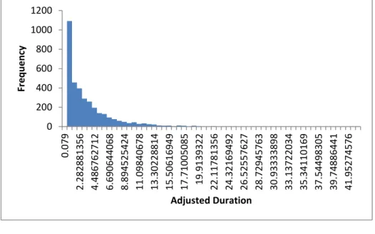
periods of each day. Figures 1 to 3 show respectively the adjusted series, the histogram of the series and the autocorrelation plot (ACF) of the series. Clearly there exist some weak but significant autocorrelations in the adjusted durations, that the ACD model will attempt to capture. The p-value for an associated Ljung-Box statistic is very close to 0.
Figure 1.Time plots of durations for US IBM stock traded in the first five trading days of November 1990: the adjusted series
0 5 10 15 20 25 30 35 40 45 50 1 14 9 29 7 44 5 59 3 74 1 88 9 10 37 11 85 13 33 14 81 16 29 17 77 19 25 20 73 22 21 23 69 25 17 26 65 28 13 29 61 31 09 32 57 34 05 A d ju ste d Du ration Sequence
Pooi Ah-Hin, Ng Kok-Haur, Soo Huei-Ching
______________________________________________________________
86
Figure 2. The histogram of the adjusted series
0 10 20 30 Lag 0.0 0.2 0.4 0.6 0.8 1.0 A CF Adjusted series
Figure 3. ACF of the adjusted series 0 200 400 600 800 1000 1200 0.0 79 2.2 8288 1356 4.4 8676 2712 6.6 9064 4068 8.8 9452 5424 11 .0984 0678 13 .3022 8814 15 .5061 6949 17 .7100 5085 19 .9139 322 22 .1178 1356 24 .3216 9492 26 .5255 7627 28 .7294 5763 30 .9333 3898 33 .13 72 20 34 35 .3411 0169 37 .5449 8305 39 .7488 6441 41 .9527 4576 Fr e q u e n cy Adjusted Duration
Modelling and Forecasting with Financial Duration Data Using Non-linear Model
87
The WACD(1,1) model and the non-linear model with l1 described in Section 3 are fitted to the first 3500 durations of transactions of IBM stock. The existing fitted WACD(1,1) model is
WACD (1,1) : xi
i
i,
i 0.12750.0576xi10.9038
i1, while the fitted non-linear model is one of which the estimated parameters are 70719 . 0 7070 . 0 7070 . 0 70719 . 0 V ,
1 3.29221,
2 3.29198,h10.97902, 93198 . 0 2 h ,
1(1) 0.14705,
(12) 0.66346,
(21) 0.47224,
(22) 0.44510, 10601 . 1 ) 1 ( 3
,
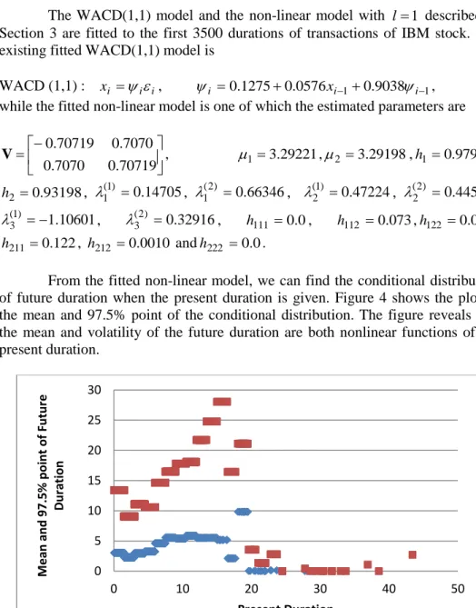
(32) 0.32916, h111 0.0, h112 0.073,h122 0.049, 122 . 0 211 h , h212 0.0010 andh222 0.0.From the fitted non-linear model, we can find the conditional distribution of future duration when the present duration is given. Figure 4 shows the plot of the mean and 97.5% point of the conditional distribution. The figure reveals that the mean and volatility of the future duration are both nonlinear functions of the present duration.
Figure 4. Plots of mean and 97.5% point of future duration against present duration 0 5 10 15 20 25 30 0 10 20 30 40 50 M e an an d 97.5% p o in t o f Fu tu re D u ration Present Duration
Pooi Ah-Hin, Ng Kok-Haur, Soo Huei-Ching
______________________________________________________________
88
Based on the above two fitted models, we calculate the in-sample MSPE and MAPD together with the out-of-sample MSFE and MAFD using the last
34
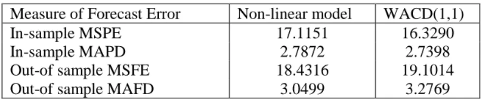
m durations. The results are shown in Table 1. The measures of forecast error shown in Table 1 show that the WACD(1,1) model gives marginally smaller in-sample MSPE/MAPD than the non-linear model, while the non-linear model gives smaller out-of-sample MSFE/MAFD than the WACD(1,1) model. Thus, the non-linear model serves as a good alternative model to the non-linear ACD model for fitting duration data.
Table 1. Results for the Non-linear and WACD(1,1) models
Measure of Forecast Error Non-linear model WACD(1,1)
In-sample MSPE 17.1151 16.3290
In-sample MAPD 2.7872 2.7398
Out-of sample MSFE 18.4316 19.1014
Out-of sample MAFD 3.0499 3.2769
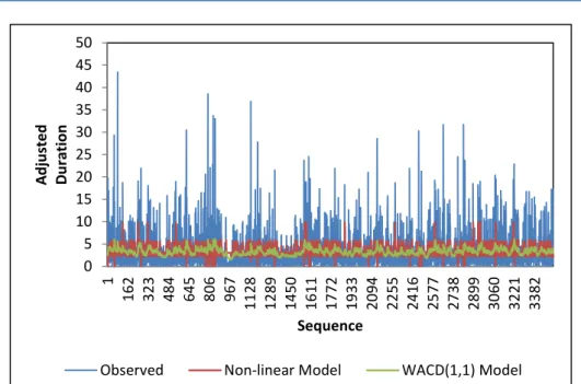
Table 2 shows the DM test statistics and their corresponding p-values. All results show that non-linear model and WACD(1,1) model have no significance difference in the forecast ability at the 5% significance level. Figure 5 graphs the fitted time series superimposed on the observed series. The results show that the non-linear and WACD(1,1) models capture the general trend, persistence and volatility clustering well. Figure 6 shows the forecasts follow the trend of the observed duration well.
Table 2: The results of the DM test for 34-step-ahead forecast, with p-values in parentheses. The benchmark is the WACD (1,1) model
Loss function based on Non-linear model Squared Error Loss -1.0248 (0.3055) Absolute Deviation Loss -1.8624 (0.0625)
Modelling and Forecasting with Financial Duration Data Using Non-linear Model
89
Figure 5.Observed x , expected t E(xt) using Non-linear model and expected )
(xt
E using WACD(1,1) model
Figure 6.Observed x , forecast t E(xt) using Non-linear model and forecast )
(xt
E using WACD(1,1) model 0 5 10 15 20 25 30 35 40 45 50 1 16 2 32 3 48 4 64 5 80 6 96 7 11 28 12 89 14 50 16 11 17 72 19 33 20 94 22 55 24 16 25 77 27 38 28 99 30 60 32 21 33 82 A d ju ste d D u ration Sequence
Observed Non-linear Model WACD(1,1) Model
0 2 4 6 8 10 12 14 16 18 20 A d ju ste d Du ration Sequence
Pooi Ah-Hin, Ng Kok-Haur, Soo Huei-Ching
______________________________________________________________
90
6.
Conclusion
This paper proposes a non-linear model for modelling the duration data. The proposed model which uses the built-in quadratic-normal distribution for the errors, does not require the user to choose a suitable error distribution. On the contrary, we need to choose a suitable distribution of the errors using the ACD models.The proposed non-linear model uses a more elaborate mechanism for specifying the non-linear mean of the distribution together with the associated variance, skewness and kurtosis whereas the linear ACD model concentrates on the variable
i for specifying the mean and dispersion of the duration.Although the results based on dataset used in this paper show that the proposed non-linear model and the linear ACD model with Weibull errorshave about the same forecast accuracy, the performance of these models may differ when we consider the multi-step ahead forecast based on other datasets. Thus future research may be carried out to further compare these two models.
Acknowledgement
The second author greatly acknowledges that this work is partially supported by the UMRG grant no: RG260-13AFR of the University of Malaya.
REFERENCES
[1] Allen, D., Ng, K.H., Peiris, S. (2013), Estimating and Simulating Weibull Models of Risk or Price Durations: An Application to ACD Models; North
American Journal of Economics and Finance, 25: 214-225;
[2] Bauwens, L., Giot, P. (2000), The Logarithmic ACD Model: An Application to the Bid-ask Quote Process of Three NYSE Stocks; AnnalesD’Economieet de
Statistique, 60: 117-145;
[3] Bauwens, L., Giot, P. (2003), Asymmetric ACD Models: Introducing Price Information in ACD Models; Empirical Economics, 28(4): 709-731;
[4] Bauwens, L., Veredas, D. (2004), The Stochastic Conditional Duration Model: A Latent Variable Model for the Analysis of Financial Durations;
Journal of Econometrics, 119(2): 381-412;
[5] Bhatti, C.R. (2010), The Birnbaum-Saunders Autoregressive Conditional Model;Mathematics and Computers in Simulation, 80(10): 2062-2078;
[6] Bollerslev, T. (1986), Generalized Autoregressive Conditional Heteroskedasticity;Journal of Econometrics, 31(3): 307-327;
[7] Diebold, F.X, Mariano, R.S. (1995), Comparing Predictive Accuracy;
Modelling and Forecasting with Financial Duration Data Using Non-linear Model
91
[8] Drost, F.C., Werker, B.J.M. (2004), Semiparametric Duration Models;
Journal of Business and Economic Statistics, 22(1): 40-50;
[9] Dufour, A., Engle, R.F. (2000), Time and the Price Impact of a Trade;
Journal of Finance, 55(6): 2467-2498;
[10] Engle, R.F., Russell, J.R. (1998), Autoregressive Conditional Duration: A New Model for Irregularly Spaced Transaction Data; Econometrica, 66(5):1127-1162;
[11] Fernandes, M., Grammig, J. (2006), A Family of Autoregressive Conditional Duration Models; Journal of Econometrics, 130(1): 1-23;
[12] Fernandes, M., Medeiros, M.C., Veiga, A. (2006),A (semi-) Parametric Functional Coefficient Autoregressive Conditional Duration Model; Texto para
Discussao;
[13] Hautsch, N. (2001), The Generalized FACD Model; Unpublished paper, University of Konstanz;
[14] Hautsch, N. (2012), Econometrics of Financial High-frequency Data; Springer;
[15] Leiva, V., Saulo, H., Leao, J., Marchant, C. (2014), A Family of Autoregressive Conditional Duration Models Applied to Financial Data;
Computational Statistics and Data Analysis, 79: 175-191;
[16] Luca, G. D., Gallo, G. M. (2008), Time-varying Mixing Weights in Mixture
Autoregressive Conditional Duration Models; Econometric Reviews, 28(1-3): 102-120;
[17] Ng, K.H., Peiris, M.S. (2013), Modelling High Frequency Transaction Data in Financial Economics: A Comparative Study based on Simulations; Economic
Computation and Economic Cybernetics Studies and Research, 47(2): 189-202;
[18] Ng, K.H., Peiris, M.S., Thavaneswaran, A., Ng, K. H. (2015), Modelling the Risk or Price Durations in Financial Markets: Quadratic Estimating Functions and Applications;Economic Computation and Economic Cybernetics
Studies and Research, 49(1): 223-238;
[19] Pacurar, M. (2008), Autoregressive Conditional Duration Models in Finance: A Survey of the Theoretical and Empirical Literature; Journal of
Economic Surveys, 22(4): 711-751;
[20] Patrick, W.S., Gao, J., Allen, D.E. (2015), Semiparametric Autoregressive Conditional Duration Model: Theory and Practice; Econometric Reviews, 34 (6-10): 849-881;
[21] Pooi, A.H. (2006), Non-normally Distributed Variates with a Nonlinear Dependence Structure; Technical Report No 13/2006, Institute of Mathematical Sciences, University of Malaya;
[22] Pooi, A.H. (2012),A Model for Time Series Analysis; Applied Mathematical
Pooi Ah-Hin, Ng Kok-Haur, Soo Huei-Ching
______________________________________________________________
92
[23] Pooi, A.H., Soo, H.C. (2013), A Test for Normality in the Presence of Outliers;JurnalTeknologi, 63(2): 95-99;
[24] Tsay, R.S. (2010), Analysis of Financial Time Series; John Wiley;
[25] Zhang, M.Y., Russell, J.R., Tsay, R.S. (2001),A Non-linear Autoregressive Conditional Duration Model with Applications to Financial Transaction Data;