doi:10.1006/jsco.1999.0416
Available online at http://www.idealibrary.com on
A Fast Algorithm for Gr¨
obner Basis Conversion and
its Applications
QUOC-NAM TRAN
Department of Computer Science, Lamar University, TX 77710, U.S.A.
The Gr¨obner walk method converts a Gr¨obner basis by partitioning the computation of the basis into several smaller computations following a path in the Gr¨obner fan of the ideal generated by the system of equations. The method works with ideals of zero-dimension as well as positive zero-dimension. Typically, the target point of the walking path lies on the intersection of very many cones, which ends up with initial forms of a consid-erable number of terms. Therefore, it is crucial to the performance of the conversion to change the target point since we have to compute a Gr¨obner basis with respect to the elimination term order of such large initial forms.
In contrast to heuristic methods found in the literature, in this paper the author presents a deterministic method to vary the target point in order to ensure the generality of the position, i.e. we always have just a few terms in the initial forms. It turns out that this theoretical result brings a dramatic speed-up in practice. We have implemented the Gr¨obner walk method together with the deterministic method for varying the target point in the kernel of Mathematica. Our experiments show the superlative performance of our improved Gr¨obner walk method in comparison with other known methods. Our best performance is 3×10⁴times faster than the direct computation of the reduced Gr¨obner
basis with respect to pure lexicographic term order (using the Buchberger algorithm and the sugar cube strategy). We also discuss the complexity of the conversion algorithm and prove a degree bound for polynomials in the target Gr¨obner basis.
In the second part of the paper, we present some applications of the conversion method for implicitization and geometric reasoning. We compare the efficiency of the improved Gr¨obner walk method with other methods for elimination such as multivariate resultant methods.
c
2000 Academic Press
1. Introduction
The method of Gr¨obner bases (Buchberger, 1965, 1985) is one of the main tools for eliminating variables and solving systems of nonlinear algebraic equations. In order to eliminate variables or to solve such a system, one has to compute a Gr¨obner basis with respect to an elimination term order, for example pure lexicographic term order. However, it is time and memory consuming to do so directly.
One way to overcome these difficulties is to partition the computation of the Gr¨obner basis into several smaller computations following a path in the Gr¨obner fan of the ideal generated by the system of equations. This approach of Collartet al.(1997) is called the “Gr¨obner walk” method, and does not require any assumption about the dimension of the ideal.
A crucial parameter of the performance of the Gr¨obner walk method is the choice of the walking path since the number of conversion steps and the complexity of each step
depend heavily on it. Ideally, the walking path should be free of the intersections of several cones since in this general position, the initial forms involve far fewer terms; therefore, the transformations can be computed cheaply. As suggested in Collartet al.(1997) and improved in Amrheinet al.(1996) and Amrhein and Gloor (1998), it is appropriate to vary the starting point in order to ensure the generality of the position.
However, the real difficulty comes from the target point, where one has to perform the last conversion with respect to the elimination term order but does not know how to vary the point. Typically, the target point lies on the intersection of very many cones, which ends up with initial forms of a considerable number of terms. (We have many examples whose initial forms have a few hundred terms.) Therefore, it increases the complexity of the conversion since we have to compute a Gr¨obner basis with respect to the elimination term order of such large initial forms. Amrhein and Gloor (1998) offer a heuristic way to guess a perturbed target point and check the validity after the conversion. But, if the heuristic guess fails then one has to compute the Gr¨obner basis with respect to the elimination term order of such large initial forms anyway.
In this paper, the author gives a deterministic method to vary the target point in order to ensure the generality of the position, i.e. we always have just a few terms in the initial forms. The main idea of the method is that, even though we do not know the Gr¨obner basis with respect to the target cone, we know in advance how large the polynomials in the Gr¨obner basis can be. More precisely, we use the upper degree bound for polynomials in the Gr¨obner basis (Bayer, 1982; Dub´e, 1990) for the variation of the target point.
It turns out that this theoretical result brings a dramatic speed-up in practice. We have implemented the Gr¨obner walk method together with the deterministic method for varying the target point in the kernel of Mathematica. Our experiments show the su-perlative performance of our improved Gr¨obner walk method in comparison with other known methods. Our best performance is 3×10⁴ times faster than the direct
computa-tion of the reduced Gr¨obner basis with respect to pure lexicographic term order (using the Buchberger algorithm and the sugar cube strategy). In Section 3.2 we discuss the complexity of the conversion algorithm. We prove that the degree of the polynomials in the target Gr¨obner basis is bounded by
22w−1d2w+ 22w+1d(n+ 1)(d+ 1)2w−2(n+ 2)2w−1−1, wherewis the length of the Gr¨obner walk.
Other approaches for basis conversion are the FGLM method for zero-dimensional systems (Faug`ere et al., 1993) and the method based on the Hilbert-Pointcar´e series (Traverso, 1996). However, in this paper we concentrate on the Gr¨obner walk method.
In the second part of the paper, we present some applications of the conversion method for implicitization and geometric reasoning. We compare the efficiency of the improved Gr¨obner walk method with other very new methods for elimination such as multivariate resultant methods.
2. Preliminaries 2.1. a degree bound
Recall that we have the following upper degree bound for polynomials in a Gr¨obner basis with respect to any admissible term order.
Lemma 2.1. (Dub´e, 1990) LetK[x1,. . .,xn]be a ring of multivariate polynomials with coefficients in a fieldK, and let F be a subset of this ring such that d is the maximum total degree of any polynomial inF. Then for any admissible term order, the total degree of polynomials in a Gr¨obner basis for the ideal generated byF is bounded by
(d2+ 2d)2n−1.
When the ideal is zero-dimensional, Caniglia et al. (1991) showed that we can even lower the degree bound todO(n).
2.2. Gr¨obner walk
In order to eliminate variables or to solve a system of nonlinear algebraic equations, one has to compute a Gr¨obner basis with respect to an elimination term order, for example pure lexicographic term order. However, it is time and memory consuming to do so directly. From the complexity point of view as well as the practical point of view, it is more efficient and requires much less memory to compute a Gr¨obner basis with respect to the degree reverse lexicographic term order in comparison with elimination term orders. Moreover, in some instances such as in implicitization of surfaces with polynomial parametric form, one knows in advance that the given set of polynomials is already a Gr¨obner basis with respect to some term orders. Therefore, it would be more efficient if one knew how to convert the known Gr¨obner basis to a Gr¨obner basis of the ideal with respect to an elimination term order.
The Gr¨obner walk method converts a Gr¨obner basis by partitioning the computation of the basis into several smaller computations following a path in the Gr¨obner fan of the ideal generated by the system of equations. The method works with ideals of zero-dimension as well as positive zero-dimension.
We now give a short introduction to basic facts and analyze the performance of the traditional algorithms for the Gr¨obner walk method. We refer to Collartet al.(1997) for missing details.
Given the reduced Gr¨obner basis of an ideal I ⊂ K[x1, . . ., xn] with respect to an admissible term order ≺1, where K is a computable field, our goal is to compute the reduced Gr¨obner basis of I with respect to another admissible term order ≺2 without applying Buchberger’s algorithm.
The set of terms in the variables x1, x2, . . . , xn is denoted by Tn. The set Ω =
{(φ1, . . . , φn) ∈ Qn : φj ≥ 0,∀1 ≤ j ≤ n} is called the set of weight vectors. Let
ω = (w1, . . . , wn) ∈ Ω; for a monomial t = cxi11x
i2 2 · · ·x
in
n , we denote its ω-degree by
degω(t) =Pn
j=1ijwj. Theω-degree of a nonzero polynomialf, denoted degω(f), is the
maximum of theω-degrees of the monomials which occur inf with nonzero coefficients. The initial form off with respect toω, denotedinω(f), is the sum of all those monomials
in f with maximal ω-degree. Furthermore, degω(0) =−1 and inω(0) = 0. We say that
≺ refines ω if degω(t1) < degω(t2) implies t1 ≺ t2 for all t1, t2 ∈ Tn. We say that ω
represents≺ifhIωi=hI≺i, whereIω={inω(f) :f ∈I} andI≺ ={in≺(f) :f ∈I}.
Lemma 2.2. (Eisenbud, 1995) Let I be an ideal, ≺ a term order and G the reduced Gr¨obner basis ofI with respect to≺. A weight vectorω represents≺forI if and only if
For the term orders≺and the weight vectorω, we define the term order (ω| ≺) by t1(ω| ≺)t2 ifdegω(t1)< degω(t2) ordegω(t1) =degω(t2) andt1≺t2.
The topological closure in Qn of {w∈ Ω :hI≺i=hIωi}, which is a convex, polyhedral cone inQn with a non-empty interior, is called the Gr¨obner cone ofIwith respect to≺. The term orders≺1 and ≺2 can be expressed by sequences of rational weight vectors S≺1 and S≺2 where their first elements, denoted byσ andτ, are weight vectors refined by≺1 and ≺2, respectively. For σ and τ in the set of weight vectors Ω, we denote the line segment in Ω betweenσandτ byστ, i.e.
στ ={(1−t)σ+tτ : 0≤t≤1}.
There exist finitely many weight vectors σ = ω0, ω1, . . ., ωm =τ in στ and pairwise
different Gr¨obner cones C≺1(I) =C0(I), C1(I) = C(ω1|≺2)(I), . . ., Cm(I) =C≺2(I) in the Gr¨obner fan ofI such that for everyk∈ {1, . . . , m}, ωk is the weight vector with
ωk−1ωk=ωk−1τ∩Ck−1(I).
We denote the reduced Gr¨obner basis ofI over the Gr¨obner coneCk(I) byGk.
We perform the Gr¨obner walk method by moving on the line segmentστ from σto τ, i.e. we computeω1,. . .,ωm−1 andG1,. . ., Gm successively. The crucial point is that
this conversion can be done efficiently without applying Buchberger’s algorithm. We first check if Ck−1(I) is equal to C≺2(I) for a given Gr¨obner basis Gk−1 = {g1, . . . , gr}. If so thenGk−1 is already the reduced Gr¨obner basis of I with respect to ≺2. Otherwise,
we have to determine the next weight vectorωk, which is the point on the segment στ
where we leave the Gr¨obner coneCk−1(I). The weight ωk can be easily computed from
ωk−1,τ andGk−1 asωk =ω(¯t) =ωk−1+ ¯t(τ−ωk−1), where
¯
t= min({t∈Q∩(0,1] : degω(t)p1= degω(t)pi,
for someg=p1+· · ·+pn∈Gk−1,2≤i≤n}). (2.1)
After leavingCk−1(I) we enterCk=C(ωk|≺2)(I). We now have to transform Gk−1to Gk. Note that there exists a term order≺which refinesωk such thatC≺(I) =Ck−1(I).
Thereforein≺(f) =in≺(inωk(f)) for allf ∈I and
hhIωki≺i=hI≺i=h(Gk−1)≺i=h((Gk−1)ωk)≺i
hence (Gk−1)ωk is the reduced Gr¨obner basis ofIωk with respect to≺. We now convert
(Gk−1)ωk to the the reduced Gr¨obner basis M = {m1, . . . , ms} of hIωki with respect
to (ωk| ≺2). Note that this conversion itself can be done with any basic conversion, for
example by using the Hilbert–Poincar´e series (Traverso, 1996) or by recursive use of the Gr¨obner walk method. However, we may want to use a specialized Buchberger’s algorithm in this case since we can perturb the weight vectors such that most of the initials are monomial. Critical pairs of two monomials are unnecessary since its S-polynomial is always zero. As most of the S-polynomials reduce to zero in one step, there is no need of sophisticated selection strategies.
Sincem1, . . . , msareωk-homogeneous, we can computeωk-homogeneous polynomials
hi1,. . .,hirwith
mi = r
X
j=1
forj= 1. . . rwithhij 6= 0. Replacinginωk(gj) bygj, we obtain fi= r X j=1 hijgj and G={f1, . . . , fs}.
It immediately follows thatinωk(fi) =mi and therefore
hI(ωk|≺2)i=hhIωki(ωk|≺2)i=hM(ωk|≺2)i=hG(ωk|≺2)i.
HenceGis a Gr¨obner basis ofI with respect to (ωk| ≺2) which we reduce toGk.
3. Main Results 3.1. a fast algorithm
As we have seen in the previous section, it is crucial to the Gr¨obner walk method to keep the initial forms as small as possible since the complexity of the method depends heavily on them. We can partly achieve this goal by varying the starting and the intermediate weight vectors to ensure that the walking path is free of the intersections of several cones. In this general position, the initial forms involve far fewer terms; therefore, the transformations can be computed cheaply. This step can be done easily since we already know the Gr¨obner basis of the cone.
However, the real difficulty comes from the target weight vector, where one has to perform the last conversion with respect to the elimination term order but does not know how to vary the point. Typically, the target point lies on the intersection of very many cones, which ends up with the initial forms of a considerable number of terms as in the following examples.
Example 3.1. Given the system of equations
5x4+ 13y2z+ 11x4yz3+ 12x2z4+ 2x4z4+ 5yz4+ 13x3yz4, 11xy+ 15y3+ 4x2y4z+ 2xz2+ 18x2z2+ 19x2yz3,
3xy+ 16xz2+ 20x3yz2+ 3yz3+ 4xy2z3+ 2x4y2z3;
we convert from a Gr¨obner basis with respect to the degree reverse lexicographic term order of the ideal generated by the system to a Gr¨obner basis with respect to the pure lexicographic term order determined byx y z. The ideal is one-dimensional. The initial forms at the target weight vector have as many as 136 terms.
Therefore, it increases the complexity of the conversion since we have to compute a Gr¨obner basis with respect to the elimination term order of such large initial forms. Amrhein and Gloor (1998) offer a heuristic way to guess a perturbed target point and check the validity after the conversion. But, if the heuristic guess fails then one has to compute the Gr¨obner basis with respect to the elimination term order of such large initial forms anyway.
Since in many problems the target term order is lexicographic, we first state and prove the main result for this special case.
. . . ,1) represents the Gr¨obner cone of I with respect to the lexicographic term order≺, wheredis an upper degree bound for polynomials in a Gr¨obner basis with respect to≺.
Proof. Even though we do not know the Gr¨obner basis of I with respect to the lexi-cographic term order≺, the existence of the Gr¨obner basis and the upper degree bound is clear (Buchberger, 1965; Bayer, 1982). In order to prove thatω represents the cone, we need to show that∀g ∈G, inω(g) =in≺(g), where Gis the reduced Gr¨obner basis
ofI with respect to ≺. The lexicographic term order can be expressed by the sequence (1,0, . . . ,0), (0,1, . . . ,0), . . ., (0,0, . . . ,1) of weight vectors. For every two monomial t1 = c1x e11 1 x e12 2 · · ·x e1n n and t2 = c2x e21 1 x e22 2 · · ·x e2n
n of g, we can assume that t1 t2;
there exists a number k, 1 ≤k ≤n such that e1k > e2k and e1j =e2j, 1 ≤j < k. If
k=nthen it is obvious that degω(t1)>degω(t2). Sincedn−ke1k ≥d
n−k(e 2k+ 1) and dn−k> dn−k−1(d−1) +dn−k−2(d−1) +· · ·+ (d−1) ≥dn−k−1e2k−1+d n−k−2e 2k−2+· · ·+e2n, we have dn−ke1k > Pn j=kd n−je
2j. Therefore degω(t1)>degω(t2), and hence inω(g) =
in≺(g),∀g∈G. 2
We now state and prove the following main result for the general case:
Theorem 3.1. For every ideal I⊂K[x1, . . .,xn] and for every admissible term order, there exists a deterministic and constructive method for finding weight vectors which represent the Gr¨obner cone of the term order.
Proof. Let≺be the term order which can be expressed by the sequence w1= (w11, w12, . . . , w1n),
w2= (w21, w22, . . . , w2n),
. . . .
wn= (wn1, wn2, . . . , wnn),
of weight vectors. LetMbe the maximum of the absolute value of all of the elements of wi, 1 ≤i≤n. Let dbe the product ofMand an upper degree bound for polynomials
in the reduced Gr¨obner basis G ofI with respect to ≺. We show that ω = (dn−1w 1+ dn−2w
2+· · ·+dwn−1+wn) represents the Gr¨obner cone of I with respect to ≺; i.e.
∀g∈G,inω(g) =in≺(g). Again, we do not know the Gr¨obner basis ofIwith respect to
the term order≺but the existence of the Gr¨obner basis and the upper degree bound is clear. For every two monomialt1=c1x
e11 1 x e12 2 . . . x e1n n andt2=c2x e21 1 x e22 2 . . . x e2n n ofg,
we can assume thatt1t2; there exists a numberk, 1≤k≤nsuch thatwk·e1> wk·e2
andwi·e1=wi·e2, 1≤i < k, wheree1= (e11, e12, . . . , e1n) ande2= (e21, e22, . . . , e2n).
Ifk=n, it is obvious that degω(t1)>degω(t2). Since wk·e1≥wk·e2+ 1, wi·e2= n X j=1 wije2j ≤ M n X j=1 e2j ≤d−1,1≤i≤n,
and n X i=k+1 dn−iwi·e2≤ n X i=k+1 dn−i(d−1)< dn−k, we have dn−kwk·e1> n X i=k dn−iwi·e2.
Therefore degω(t1)>degω(t2); henceinω(g) =in≺(g),∀g∈Gand we are done.2
Remark. (1) The degree bound computation is based on the original system of equa-tions.
(2) For the starting point and the intermediate weight vectors, the degree bound is the actual highest degree of the polynomials in the known reduced Gr¨obner basis. (3) Theorem 3.1 is still correct for maximal Gr¨obner bases.
Corollary 3.1. For every idealI⊂K[x1,. . .,xn]and for every pair of two admissible term orders, there exists a deterministic and constructive method based on the upper degree bound for finding an appropriate target point; i.e. we are able to find a weight vector which represents the target cone.
Based on the previous theorem, we propose a fast algorithm for basic conversion as follows.
Algorithm 3.1.
Inputs: The reduced Gr¨obner basisG1of an idealIwith respect to an arbitrary
admis-sible term order≺1 and a second term order≺2; the unique weight vectorsσ and τ (up to a scalar factor) refined by≺1 and≺2 respectively.
Output: The reduced Gr¨obner basis G2 ofI with respect to≺2.
(1) G←G1.
(2) Find a new starting point ifσlies on the intersection of several cones. (3) While True
(a) Find the next weight vectorω (b) Ifω=τ
(i) IfGis also the Gr¨obner basis ofI with respect to≺2,returnG.
(ii) Else find a new target point if τ lies on the intersection of several cones;
continue.
(c) Convert theω-initial Gr¨obner basis to the reduced Gr¨obner basis with respect to (ω| ≺2).
(d) Lift theω-initial Gr¨obner basis to the full Gr¨obner basis with respect to (ω| ≺2). The termination and correctness of the algorithm are obvious from the Gr¨obner walk method and Theorem 3.1. Note that we can even change the path during the walk, i.e. if the intermediate weight vectorω is on the intersection of several cones, we can find a new weight vectorω0 such thatω0 represents (ω0| ≺2).
3.2. a degree bound for the conversion algorithm
In this section we assume thatI be a homogeneous ideal inK[x0,x1,. . .,xn], where
x0 is the homogenous variable.
LetF andGbe two adjacent reduced Gr¨obner bases of I; i.e. the intersection of the Gr¨obner cone of F and the Gr¨obner cone of Ggenerates ann-dimensional subspace in Qn+1. It has been shown in Kalkbrener (1999) that the degree of polynomials in G is bounded by
2d2+ (n+ 1)d, (3.2)
where d = max({deg(f)|f ∈ F}). Additionally, Theorem 3.1 gives us a mechanism to assure that we always walk between the adjacent Gr¨obner cones.
Letwbe the length of the Gr¨obner walk (Algorithm 3.1) from C≺1(I) toC≺2(I). We prove the following bound.
Lemma 3.2. The degree of polynomials in the reduced Gr¨obner basisG2 ofI with respect
to≺2 is bounded by
Bw= 22
w
−1d2w
+ 22w+1d(n+ 1)(d+ 1)2w−2(n+ 2)2w−1−1.
Proof. From the recursive function (3.2), it is easy to see that the boundBw can be
written in the form
Bw=Dw+d(n+ 1)Fw,
whereDw= 22
w
−1d2w
.
We now prove that theFw is bounded by 22
w+1
(d+ 1)2w−2(n+ 2)2w−1−1 by induction
on the length w of the Gr¨obner walk. It is obvious for w = 1. Assume that Fk−1 is
bounded by 22k(d+ 1)2k−1−2(n+ 2)2k−2−1. Since Fk= 2d(n+ 1)Fk2−1+ 4Dk−1Fk−1+ Dk−1 d + (n+ 1)Fk−1, we have Fk≤2d(n+ 1)[22 k (d+ 1)2k−1−2(n+ 2)2k−2−1]2+ 4×22k−1−1d2k−122k(d+ 1)2k−1−2(n+ 2)2k−2−1+ 22k−1−1d2k−1−1+ (n+ 1)22k(d+ 1)2k−1−2(n+ 2)2k−2−1. Therefore Fk≤2d(n+ 1)22 k+1 (d+ 1)2k−4(n+ 2)2k−1−2+ (d+ 1)222k+1(d+ 1)2k−4(n+ 2)2k−1−2+ d2(n+ 1)22k+1(d+ 1)2k−4(n+ 2)2k−1−2+ (n+ 1)22k+1(d+ 1)2k−4(n+ 2)2k−1−2 = 22k+1(d+ 1)2k−2(n+ 2)2k−1−1. 2
3.3. implementation
We have implemented Algorithm 3.1 in the kernel of Mathematica. The implemented function is designed so that the users can control several parameters (options) for the conversion. Among the parameters are:
• ConvertOnly -> False/True, which tells the function to compute or not to com-pute the Gr¨obner basis with respect to the first term order,
• Perturbation -> True/False, which tells the function to use or to skip the per-turbation (varying) of the weight vectors.
• MaximalGroebnerBasis -> False/True, which tells the function to work with maximal or reduced Gr¨obner bases.
The following examples show the efficiency of the fast algorithm for basis conversion presented in the previous section. All the experiments were carried out on a laptop PC using Linux Redhat 5.0 on an Intel MMX-233 MHz processor with 144 MB RAM. Example 3.2. (ISSAC system challenge 1997) Given the zero-dimensional system of equations 8w2+ 5wx−4wy+ 2wz+ 3w+ 5x2+ 2xy−7xz−7x+ 7y2 −8yz−7y+ 7z2−8z+ 8, 3w2−5wx−3wy−6wz+ 9w+ 4x2+ 2xy−2xz+ 7x+ 9y2 +6yz+ 5y+ 7z2+ 7z+ 5, −2w2+ 9wx+ 9wy−7wz−4w+ 8x2+ 9xy−3xz+ 8x+ 6y2 −7yz+ 4y−6z2+ 8z+ 2, 7w2+ 5wx+ 3wy−5wz−5w+ 2x2+ 9xy−7xz+ 4x−4y2 −5yz+ 6y−4z2−9z+ 2;
we convert from a Gr¨obner basis with respect to the degree reverse lexicographic term order of the ideal generated by the system to a Gr¨obner basis with respect to the pure lexi-cographic term order determined byxyzw. The initial forms at the target weight vector have as many as 17 terms. Using the improved method in this paper, the conver-sion took 5.33 s while the traditional Gr¨obner walk method did not stop after 10 000 s, which is even worse than the direct computation of the Gr¨obner basis using Buchberger’s algorithm and the sugar cube strategy. (The direct computation took 159 s.)
Example 3.3. Given the system of equations 16 + 3x3+ 16x2z+ 14x2y3,
6 +y3z+ 17x2z2+ 7xy2z2+ 13x3z2
we convert from a Gr¨obner basis with respect to the degree reverse lexicographic term order of the ideal generated by the system to a Gr¨obner basis with respect to the pure lexicographic term order determined byx y z. The ideal is one-dimensional. The initial forms at the target weight vector have as many as 44 terms. Using the improved method in this paper, the conversion took 91.07 s while both the traditional Gr¨obner walk method and the direct computation of the Gr¨obner basis using Buchberger’s algorithm and the sugar cube strategy did not stop after 10 000 s.
c
d a
b
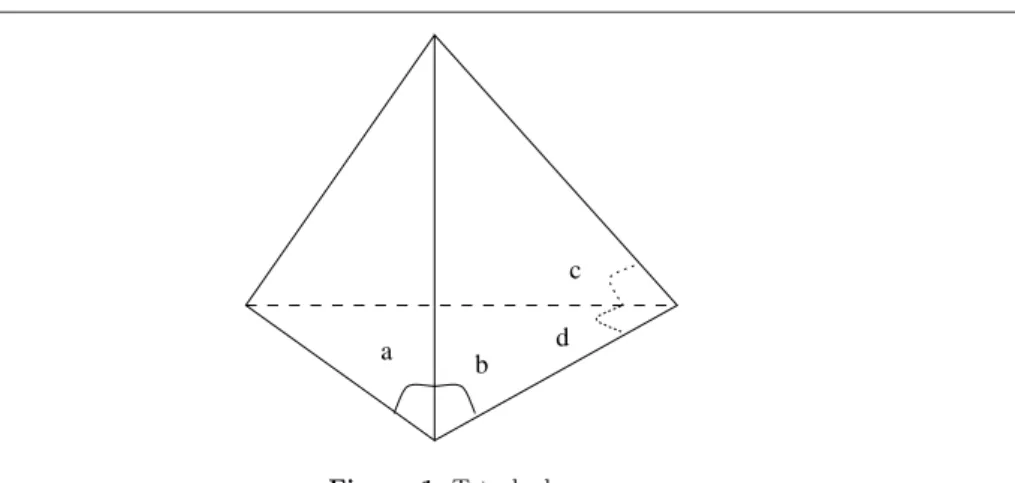
Figure 1.Tetrahedron.
The fast algorithm for basis conversion in this paper so far has the best performance of 3×10⁴ times faster in comparison with the direct computation of the Gr¨obner basis
using Buchberger’s algorithm and the sugar cube strategy in the following example. Example 3.4. Given the system of equations
15 + 10x2y2+ 13yz+ 14xy2z+ 8x2yz2+ 11xy3z2, 5 + 4xy+ 8y2,
16x3+ 19y+ 4x2y,
we convert from a Gr¨obner basis with respect to the degree reverse lexicographic term order of the ideal generated by the system to a Gr¨obner basis with respect to the pure lexicographic term order determined by x y z. The initial forms at the target weight vector have as many as 13 terms. Using the improved method in this paper, the conversion took 0.93 s, while the direct computation of the Gr¨obner basis using Buchberger’s algorithm and the sugar cube strategy took 28 518 s.
4. Some Applications of the Method for Basis Conversion 4.1. geometric reasoning
Several problems in geometric reasoning can be transformed into variable elimination problems. However, the problems usually involve parameters, i.e. the ideal generated by the system of equations may be neither zero-dimensional nor a hypersurface. One of the strong points of the Gr¨obner walk method is that it is not restricted by any assumptions on the dimension of the ideal.
In contrast to multivariate resultant methods such as the Dixon resultant method, the method of Gr¨obner bases does not have any problem with extraneous solutions; in fact, it can be used for solving the problems in full generality.
Example 4.1. The problem is to compute the maximum volume that a tetrahedron can have in terms of the areas a, b, c andd of its faces. A straightforward approach using Lagrange multipliers, would lead to a system of 12 equations in 16 variables, which is too large even for computing a Gr¨obner basis with respect to the degree reverse lexicographic
term order. Fortunately, Gerber (1975) showed that if there exist parametersx,y,z and wsatisfying the equations
yz+zw+wy−a, zx+xw+wz−b, wx+xy+yw−c, xy+yz+zx−d,
2(xyz+yzw+zwx+wxy)−9T,
then the tetrahedron is orthocentric and therefore has the maximum volume with those face areas.
In Kapur (1998) the problem was deemed not easily solvable by any method but Dixon resultant. In that paper, the author reported that the problem can be solved in 76 s on a Sun workstation using the Dixon resultant method. Using the improved Gr¨obner walk method in this paper, we can solve the problem in 12 s on a laptop PC with an Intel MMX-233 MHz processor. Moreover, the solution is fully general; it is a quartic polynomial in T2of 434 terms and we are able to write down a radical formula forT in terms of a,b, candd.
4.2. intersection of surfaces and implicitization
Designing curves and surfaces plays an important role in the construction of many products such as airplane fuselages and wings, ship hulls, propeller blades, car bodies, shoe insoles and bottles. The subject is studied in several research areas such as computer aided geometric design (CAGD), visualization and solid modeling, where curves and surfaces are approximated, represented and processed by a computer. In these domains, finding the intersection of two surfaces is a fundamental and difficult problem.
Intersections are needed to build and interrogate models of complex shapes in the computer. They are primarily used to evaluate set operations on primitive volumes in creating boundary representations of complex objects or for subsequent manipulation of the objects.
Due to the importance of the problem, there have been persistent efforts at devising algorithms for this problem (see Barnhillet al., 1987; Bajajet al., 1988; Hoffmann, 1989; Patrikalakis, 1993; Tran, 1995). The main issue in the problem is the efficient discovery and description of all features of the solution with high precision commensurate with the tasks required from the underlying geometric modeler. Reliability and efficiency of intersection algorithms are two basic prerequisites for their effective use in any geometric modeling system. They are closely associated with the way the algorithm handles such features as near singular cases, small loops, etc.
Since parametric form is the most common representation of surfaces in CAGD, solid modeling, etc. (because of its convenient manner for generating points along curves or surfaces), we first start with finding the intersection of two parametric surfaces.
Given two parametric surfacesS1 andS2 inC3 defined by the systems S1= x=u1(s1,t1) r1(s1,t1), y= v1(s1,t1) r1(s1,t1), z= w1(s1,t1) r1(s1,t1) , S2= x=u2(s2,t2) r2(s2,t2), y= v2(s2,t2) r2(s2,t2), z= w2(s2,t2) r2(s2,t2) ,
one needs to find a closed form expression for the intersection, which can be used for subsequent manipulation. But, whereas two (relatively prime) plane curves intersect in some finite number of isolated points, two surfaces meet in a space curve comprised of finitely many components.
It is well-known that the closed form expression of the intersection can be obtained by: first, implicitizing the first parametric surface S1 getting an implicit equation, say f1(x, y, z); second, substituting the parametric expression of the second surfaceS2 into
the implicit equationf1(x, y, z). This results in the implicit representation f1(x(s2, t2), y(s2, t2),z(s2, t2)) of the intersection curve in a parameter space, i.e. a projected image
of the intersection.
Implicitization is an elimination problem, even though for some time it has been deemed as unsolvable in CAD literature. Sederberg and Anderson (1984) presented a solution of the implicitization problem using resultants. The solution is spelled out for surfaces in three dimensions and curves in two dimensions. However, in the general case, except for the traditional resultant system method (van der Waerden, 1940), which is very inefficient, other conditional multivariate resultants such as Dixon’s resultant can yield only one implicit equation (e.g. implicitization of a space curve may have two or more equations) and may introduce nontrivial extraneous solutions. Arnon and Seder-berg (1984) have shown how the method of Gr¨obner bases (Buchberger, 1965, 1985) can be used for the implicitization problem of (n−1)-dimensional hypersurfaces.
There were concerns (e.g. Buchberger, 1986; Hoffmann, 1993) about the efficiency of the method of Gr¨obner bases for elimination in terms of computation time as well as memory used for the computation. Fortunately, there have been extensive improvements of the method over the last 10 years. For example, Hoffmann (1989) has shown how to use the strategy of the FGLM-algorithm for the implicitization problem of (n−1)-dimensional hypersurfaces. Moreover, in some instances, such as in implicitization of surfaces with polynomial parametric form, one knows in advance that the given set of polynomials is already a Gr¨obner basis with respect to some term orders. Therefore, it would be more efficient if one knew how to convert the known Gr¨obner basis to a Gr¨obner basis of the ideal with respect to an elimination term order. By using a new algorithm for basis conversion for non-zero dimensional systems together with an elimination term order, we can implicitize the first surface of Example 4.2 (see below) in 0.7 s using 0.5 MB on a Sun Ultrasparc-5 machine. Meanwhile, the same surface cannot be parametrized in 85 500.0 s after consuming 512 MB memory using Buchberger’s algorithm with lexicographic term order.
LetKbe an algebraically closed field. We consider the general implicitization problem for rational parametric surfaces.
Problem 4.1. (General implicitization)
Given: a surface in parametric formS ≡(xi = pqi((ss1,...,sm)
1,...,sm), wherepi, q∈K[s1, . . . , sm],
i= 1, . . . , n).
Find: f1, . . . , fk ∈K[x1, . . . , xn] such that the algebraic setV(I)≡ {(x1,. . ., xn)|fi(x1, . . ., xn) = 0, i = 1, . . . , k} is the smallest algebraic set in Kn that contains the
imageS of the parametrization.
In order to deal with the base points, one can either make use of an ingenious trick by adding one more equation qt−1 into the system, wheret is a new variable, or embed
the surface into the projective space. More theoretical details can be found in Coxet al.
(1996).
The problem requires constructing k polynomials implicitly defining hypersurfaces whose intersection is the smallest algebraic set containing the image described by the parametric representation.
It is worth mentioning that the algebraic set V(I) is irreducible. In order to comply with the degree of the implicitization, one may have to embed the algebraic set into the projective space (Hoffmann, 1989). In this case, the corresponding algebraic set is still (projectively) irreducible.
Algorithm 4.1. (Implicitization)
GB =Gr¨obnerBasis({x1q−p1, . . . , xnq−pn, qt−1}) a Gr¨obner basis with respect to
an elimination term order determined bytsixj ∀i= 1. . . m, j= 1. . . n.
{f1, . . . , fk}= GB∩K[x1, . . . , xn].
Note that since we assume the base field is algebraically closed, the differences between the algebraic setV(I) defined by the implicit equations and the imageSof the parametric surface are unions of some lower-dimensional algebraic sets, e.g. curves on a surface or points on a curve. Unfortunately, the property is not preserved for non-algebraically closed fields such asRas shown by the following counter-example. LetS= (u2, v2, uv)⊂ R3thenV(I) =V(z2−xy). However, S covers only half ofV(I).
We can now state the problem of intersection of parametric surfaces and generalize it to higher dimensions as follows.
Problem 4.2. (Intersection of parametric surfaces) Given: two parametric surfaces S1 = (xi = pq1i(s11,...,s1m)
1(s11,...,s1m), where p1i, q1 ∈ K[s11, . . .,
s1m], i= 1, . . . , n), and S2= (xi =
p2i(s21,...,s2m)
q2(s21,...,s2m), wherep2i, q2 ∈K[s21,. . . , s2m],
i= 1, . . . , n).
Find: a closed form expression for the intersection ofS1 andS2.
The closed form expression for the intersection can be the projected image of the inter-section onto the parameter space of either of the two given surfaces.
Algorithm 4.2. (Intersection of parametric surfaces)
F1={f1, . . . , fk} ⊂K[x1, . . . , xn], an implicitization of the surfaceS1. F1=F1|x
i←pq22 (i(ss2121,...,s,...,s22mm)),∀i=1,...,n
Example 4.2. Given two tensor product surfaces, where the first one is the airplane wing-shape surface q1= (1−u)(1−v)4+ 40(1−u)v(1−v)3+ 120(1−u)v2(1−v)2 +40(1−u)v3(1−v) + (1−u)v4+u(1−v)4+ 40uv(1−v)3 +120uv2(1−v)2+ 40uv3(1−v) +uv4; x= 1 q1 (60u(1−v)4+ 2400uv(1−v)3+ 7200uv2(1−v)2+ 2400uv3
-4-20 2 4 0 25 50 75 -5 0 5 10 -4-20 2 4 0 25 50 75 0 20 40 600 10 20 3002 4 0 20 40 60 0 0 5 10 15 0 25 50 75 -5 0 5 10 0 5 10 0 25 50 75
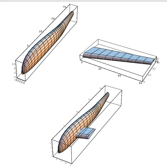
Figure 2.Intersections of parametric surfaces.
(1−v) + 60uv4); y= 1 q1 (20(1−u)(1−v)4+ 160(1−u)v(1−v)3+ 160(1−u)v3(1−v) +20(1−u)v4+ 30u(1−v)4+ 880uv(1−v)3+ 2400uv2(1−v)2 +880uv3(1−v) + 30uv4); z= 31 q1 ((1−u)(1−v)4+ 280(1−u)v(1−v)3+ 360(1−u)v2(1−v)2 −40(1−u)v3(1−v) + 3(1−u)v4+ 3u(1−v)4+ 200uv(1−v)3 +360uv2(1−v)2+ 40uv3(1−v) + 3uv4);
and the second one is the airplane fuselage-shape surface
q2= (1−u)3(1−v)5+ 10(1−u)3v(1−v)4+ 30(1−u)3v2(1−v)3
+30u(1−u)2(1−v)5+ 300u(1−u)2v(1−v)4+ 900u(1−u)2 v2(1−v)3+ 900u(1−u)2v3(1−v)2+ 300u(1−u)2v4(1−v) +30u(1−u)2v5+ 30u2(1−u)(1−v)5+ 300u2(1−u)v(1−v)4 +900u2(1−u)v2(1−v)3+ 900u2(1−u)v3(1−v)2+ 300u2 (1−u)v4(1−v) + 30u2(1−u)v5+u3(1−v)5+ 10u3v(1−v)4 +30u3v2(1−v)3+ 30u3v3(1−v)2+ 10u3v4(1−v) +u3v5; x= 1 q2 (−12.50(1−u)3v(1−v)4−37.50(1−u)3v2(1−v)3+ 37.50 (1−u)3v3(1−v)2+ 12.50(1−u)3v4(1−v)−1650u(1−u)2v (1−v)4−4950u(1−u)2v2(1−v)3+ 4950u(1−u)2v3 (1−v)2+ 1650u(1−u)2v4(1−v)−1650u2(1−u)v(1−v)4 −4950u2(1−u)v2(1−v)3+ 4950u2(1−u)v3(1−v)2+ 1650 u2(1−u)v4(1−v)−25u3v(1−v)4−75u3v2(1−v)3+ 75u3v3 (1−v)2+ 25u3v4(1−v)); y= 1 q2 (−20(1−u)3(1−v)5−200(1−u)3v(1−v)4−600(1−u)3v2 (1−v)3−600(1−u)3v3(1−v)2−200(1−u)3v4(1−v)−20 (1−u)3v5−420u(1−u)2(1−v)5−4200u(1−u)2v(1−v)4 −12600u(1−u)2v2(1−v)3−12600u(1−u)2v3(1−v)2−4200 u(1−u)2v4(1−v)−420u(1−u)2v5+ 1500u2(1−u)(1−v)5 +15000u2(1−u)v(1−v)4+ 45000u2(1−u)v2(1−v)3+ 45000 u2(1−u)v3(1−v)2+ 15000u2(1−u)v4(1−v) + 1500u2(1−u) v5+ 80u3(1−v)5+ 800u3v(1−v)4+ 2400u3v2(1−v)3+ 2400 u3v3(1−v)2+ 800u3v4(1−v) + 80u3v5); z= 1 q2 (−(1−u)3(1−v)5−10(1−u)3v(1−v)4+ 60(1−u)3v2(1−v)3 +60(1−u)3v3(1−v)2−10(1−u)3v4(1−v)−(1−u)3v5 −150u(1−u)2(1−v)5−1500u(1−u)2v(1−v)4+ 11700u (1−u)2v2(1−v)3+ 11700u(1−u)2v3(1−v)2−1500u(1−u)2v4 (1−v)−150u(1−u)2v5−150u2(1−u)(1−v)5−1500u2(1−u) v(1−v)4+ 11700u2(1−u)v2(1−v)3+ 11700u2(1−u)v3(1−v)2 −1500u2(1−u)v4(1−v)−150u2(1−u)v5+ 4u3(1−v)5+ 40u3 v(1−v)4+ 321u3v2(1−v)3+ 321u3v3(1−v)2+ 40u3v4(1−v) +4u3v5);
We first implicitize the wing-shape surface using a new algorithm for basis conversion for non-zero dimensional systems together with an elimination term order. The computation has been done in 0.7 s using 0.5 MB on a Sun Ultrasparc-5 machine. The implicitization representation of the wing-shape surface is an irreducible polynomial inx,yandz, which has degree 8 and consists of 143 terms. Simply substituting the parametric expression of the fuselage-shape surface into the implicitization representation of the wing-shape
surface we get a closed form expression for the intersection, which is a projected image of the intersection onto the parameter space of the wing-shape surface. The closed form expression is a rational function inuandvwhose numerator has degree 88 and consists of 2009 terms. The denominator is of degree 11 and consists of 30 terms.
5. Conclusion
We presented a deterministic and constructive method for varying the target point in order to ensure the generality of its position, a crucial condition to the performance of the Gr¨obner walk method for basis conversion. We showed a fast algorithm for basis conversion and its implementation in the kernel of Mathematica. Our experiments show the superlative performance of our improved Gr¨obner walk method in comparison with other known methods. Our best performance is 3×10⁴ times faster than the direct
computation of the reduced Gr¨obner basis with respect to pure lexicographic term order (using the Buchberger algorithm and the sugar cube strategy). Finally, we reported the practical value of our algorithm for some problems in CAGD and geometric reasoning.
References
Amrhein, B., Gloor, O. (1998). The fractal walk. In Buchberger, B., Winkler, F. eds,Proceedings of the Conference “33 Years of Gr¨obner Bases”, Linz. Cambridge, UK, Cambridge University Press. Amrhein, B., Gloor, O., K¨uchlin, W. (1996). Walking faster. InProceedings of the DISCO’96, Karlsruhe,
Germany. Berlin, Springer-Verlag.
Arnon, D., Sederberg, T. (1984). Implicit equation for a parametric surface by Gr¨obner basis. In Pro-ceedings of 1984 MACSYMA User’s Conf., pp. 431–436. New York, USA, Schenectady.
Bajaj, C. L., Hoffmann, C. M., Lynch, R. E., Hopcroft, J. E. H. (1988). Tracing surface intersections. Comput. Aided Geom. Des.,5, 285–307.
Barnhill, R., Farin, G., Jordan, M., Piper, B. (1987). Surface/surface intersection.Comput. Aided Geom. Des.,4, 3–16.
Bayer, D. (1982). The division algorithm and the Hilbert scheme. Ph.D. Thesis, Harvard University, Cambridge.
Buchberger, B. (1965). An algorithm for finding a basis for the residue class ring of a zero-dimensional polynomial ideal (in German). Ph.D. Thesis, Institute of Mathematics, Univ. Innsbruck, Innsbruck, Austria.
Buchberger, B. (1985). Gr¨obner bases: An algorithmic method in polynomial ideal theory. In Bose, N. K. ed.,Multidimensional Systems Theory, chapter 6, pp. 184–232. Dodrecht, Reidel Publishing Company.
Buchberger, B. (1986). What can Gr¨obner bases do for computational geometry and robotics. In Pro-ceedings of Workshop on Geometric Reasoning, Oxford, England.
Caniglia, L., Galligo, A., Heintz, J. (1991). Equations for the projective closure and effective nullstellen-satz.Discrete Appl. Math.,33, 11–23.
Collart, S., Kalkbrener, M., Mall, D. (1997). Converting bases with the Gr¨obner walk.J. Symb. Comput., 24, 465–469.
Cox, D., Little, J., O’Shea, D. (1996). InIdeals, Varieties, and Algorithms: An Introduction to Com-putational Algebraic Geometry and Commutative Algebra, Undergraduate Texts in Mathematics, 2nd
edn. New York, Springer-Verlag.
Dub´e, T. D. (1990). The structure of polynomial ideals and Gr¨obner bases.SIAM J. Comput.,19, 750–773.
Eisenbud, D. (1995).Commutative Algebra with a View Towards Algebraic Geometry, volume 150 of Graduate Texts in Mathematics. New York, Springer.
Faug`ere, F. C., Gianni, P., Lazard, D., Mora, T. (1993). Efficient computation of zero-dimensional Gr¨obner bases by change of ordering.J. Symb. Comput.,16, 329–344.
Gerber, L. (1975). The orthocentric simplex as an extreme simplex.Pac. J. Math.,56, 97–111. Hoffmann, C. (1989).Geometric and Solid Modeling—An Introduction. San Mateo, California, Morgan
Kaufmann Publishers, Inc..
Hoffmann, C. (1993). Implicit curves and surfaces in CAGD.IEEE Comput. Graph. Appl.,13, 79–88. Kalkbrener, M. (1999). On the complexity of Gr¨obner bases conversion.J. Symb. Comput.,28, 265–274. Kapur, D. (1998). Automated geometric reasoning: Dixon resultants, Gr¨obner bases and characteristic sets. In Wang, D. ed.,Automated Deduction in Geometry, volume 1360 ofLecture Notes in Artifi-cial Intelligent. pp. 1–36. Springer.
Patrikalakis, N. M. (1993). Surface-to-surface intersections.IEEE Comput. Graph. Appl.,1, 89–95. Sederberg, T. W., Anderson, D. C. (1984). Implicit representation of parametric curves and surfaces.
Computer Vison, Graphics and Image Processing,28, 72–84.
Tran, Q.-N. (1995). A hybrid symbolic-numerical method for tracing surface-to-surface intersections. In The proceedings of ISSAC’95, pp. 51–58. Montreal, Canada.
Traverso, C. (1996). Hilbert functions and the Buchberger algorithm.J. Symb. Comput.,22, 355–376. van der Waerden, B. L. (1940).Moderne Algebra, volume 2, 2ndedn. Berlin, Springer-Verlag.
Originally Received 31 January 1999 Accepted 22 June 1999