Interest Rate Modeling and Forecasting in India

(1)

CDE July 2004

Centre for Development Economics

Interest Rate Modeling and

Forecasting in India

Pami Dua

Department of Economics, Delhi School of Economics, Delhi, India and Economic Cycle Research Institute, New York

Fax: 91-11-27667159 Email : dua@econdse.org

Nishita Raje

Satyananda Sahoo

Department of Economic Analysis and Policy Reserve Bank of India

Mumbai Fax: 022-2261-0626 Email : nbraje@rbi.org.in ssahoo@rbi.org.in

Abstract

The study develops univariate (ARIMA and ARCH/GARCH) and multivariate models (VAR, VECM and Bayesian VAR) to forecast short- and long-term rates, viz., call money rate, 15-91 days Treasury Bill rates and interest rates on Government securities with (residual) maturities of one year, five years and ten years. Multivariate models consider factors such as liquidity, Bank Rate, repo rate, yield spread, inflation, credit, foreign interest rates and forward premium. The study finds that multivariate models generally outperform univariate ones over longer forecast horizons. Overall, the study concludes that the forecasting performance of Bayesian VAR models is satisfactory for most interest rates and their superiority in performance is marked at longer forecast horizons.

This paper was earlier published in November 2003 as Development Research Group Study No. 24 under the aegis of the Reserve Bank of India. Permission to publish the study in its present form has been obtained from the Reserve Bank of India.

(2)

Acknowledgements

We are deeply indebted to Dr. Y. V. Reddy, then Deputy Governor, for giving us the opportunity to undertake the project on “Interest Rate Modelling and Forecasting in India”. Special thanks are also due to Dr. Rakesh Mohan, Deputy Governor, for his keen interest in the project.

We are also very grateful to Dr. Narendra Jadhav, Principal Adviser, Department of Economic Analysis and Policy (DEAP), for insightful discussions and support throughout the project. We also gratefully acknowledge and appreciate invaluable help and support from Shri. Somnath Chatterjee, Director, DEAP. His meticulous attention to administrative formalities greatly facilitated the completion of the project. We extend our thanks also to Smt. Balbir Kaur, Director, DEAP, New Delhi, for her support and guidance in the initial stages of the project.

The Study was presented at a seminar in the Reserve Bank of India. We are thankful to the discussants, S/Shri. B.K.Bhoi, Indranil Sengupta and Indranil Chakraborty, as well as other participants for their invaluable comments. We also thank the staff of DRG, Smt. A. A. Aradhye, Smt. Christine D’Souza, Shri N.R. Kotian and Shri B.S. Gawas for extending the necessary help.

We also gratefully acknowledge useful discussions that the external expert had with Nitesh Jain, Gaurav Kapur, and Jitendra Keswani in the initial stages of the project. Finally, we are extremely grateful to Sumant Kumar Rai for competent and skilled research assistance.

(3)

EXECUTIVE SUMMARY

The interest rate is a key financial variable that affects decisions of consumers, businesses, financial institutions, professional investors and policymakers. Movements in interest rates have important implications for the economy’s business cycle and are crucial to understanding financial developments and changes in economic policy. Timely forecasts of interest rates can therefore provide valuable information to financial market participants and policymakers. Forecasts of interest rates can also help to reduce interest rate risk faced by individuals and firms. Forecasting interest rates is also very useful to central banks in assessing the overall impact (including feedback and expectation effects) of its policy changes and taking appropriate corrective action, if necessary. In fact, the usefulness of the information contained in interest rates greatly increases following financial sector liberalisation.

In the Indian context, the progressive deregulation of interest rates across a broad spectrum of financial markets was an important constituent of the package of structural reforms initiated in the early 1990s. As part of this process, the Reserve Bank has taken a number of initiatives in developing financial markets, particularly in the context of ensuring efficient transmission of monetary policy.

Against this backdrop, the objective of this study is to develop models to forecast short-term and long-term rates: call money rate, 15-91 days Treasury bill rate and rates on 1-year, 5-years and 10-years government securities. Univariate as well as multivariate models are estimated for each interest rate. Univariate models include Autoregressive Integrated Moving Average (ARIMA) models, and ARIMA models with Autoregressive Conditional Heteroscedasticity (ARCH)/Generalised Autoregressive Conditional Heteroscedasiticity (GARCH) effects while multivariate models include Vector Autoregressive (VAR) models specified in levels, Vector Error Correction Models (VECM), and Bayesian Vector Autoregressive (BVAR) models. In the multivariate models, factors such as liquidity, bank rate, repo rate, yield spread, inflation, credit, foreign interest rates and forward premium are considered. The random walk model is used as the benchmark for evaluating the forecast performance of each model.

(4)

Evaluation of Forecasting Models

For each interest rate, a search for the “best” forecasting model is conducted. The “best model” is defined as one that produces the most accurate forecasts such that the predicted levels are close to the actual realized values. Furthermore, the predicted variables should move in the same direction as the actual series. In other words, if a series is rising (falling), the forecasts should reflect the same direction of change. If a series is changing direction, the forecasts should also identify this. To select the best model, the alternative models are initially estimated using weekly data over the period April 1997 through December 2001 and out-of-sample forecasts up to 36-weeks-ahead are made from January through September 2002. In other words, by continuously updating and reestimating, a real world forecasting exercise is conducted to see how the models perform.

Main Findings for Each Interest Rate

The variables employed in the multivariate models as well as the specific conclusions with respect to the various interest rates are given below.

♦ Call money rate

• The multivariatemodels for the call money rate include the following: inflation rate

(week-to-week), bank rate, yield spread, liquidity, foreign interest rate (3-months Libor), and forward premium (3-months).

• Evaluation of out-of-sample forecasts for the call money rate suggests that an

ARMA-GARCH model is best suited for very short-term forecasting while a BVAR model with a loose prior can be used for longer-term forecasting.

♦ Treasury Bill rate (15-91 days)

The following variables are included in the multivariate models for the Treasury Bill rate (15-91 days): inflation rate (year-on-year), bank rate, yield spread, liquidity, foreign interest rate (3-months Libor), and forward premium (3-(3-months).

• In the case of the 15-91 day Treasury Bill rate, the VAR model in levels produces the

most accurate short- and long-term forecasts.

♦ Government Security 1 year

• The multivariate models for 1 year government securities utilize the following variables:

inflation rate (year-on-year), bank rate; yield spread, liquidity, foreign interest rate (6-months Libor), forward premium (6-months).

• The performance of the out-of-sample forecasts for 1-year government securities

(5)

♦ Government Security 5 years

• The multivariate models for 5 years government securities include the following:

inflation rate (year-on-year), bank rate; yield spread, credit, foreign interest rate (6-months Libor), and forward premium (6-months).

• For 5-year government securities, the BVAR models do not perform well. Overall,

VECM outperforms all the alternative models. VECM also generally outperforms the alternatives at the short and long run forecast horizons.

♦ Government Security 10 years

• The following variables are used in the multivariate models for 10 years government

securities: inflation rate (year-on-year), bank rate, yield spread, credit, foreign interest rate (6-months Libor), and forward premium (6-months).

• The forecasting performance of all the models is satisfactory for 10-year government

securities. The model that produces the most accurate forecasts is a VAR in levels (LVAR); in other words, a BVAR with a very loose prior. The LVAR model also produces the most accurate short- and long-term forecasts.

The selected models conform to expectations. Standard ARIMA models are based on a constant residual variance. Since financial time series are known to exhibit volatility clustering, this effect is taken into account by estimating ARCH/GARCH models. It is found that although the ARCH/GARCH effects are significant, the ARCH model produces more accurate out-of-sample forecasts relative to the corresponding ARIMA model only in the case of call money rate. This result is not surprising since the out-of sample period over which the alternative models are evaluated is relatively stable with no marked swing in the interest rates.

It is also found that the multivariate models generally produce more accurate forecasts over longer forecast horizons. This is because interactions and dependencies between variables become stronger for longer horizons. In other words, for short forecast horizons, predictions that depend solely on the past history of a variable may yield satisfactory results.

In the class of multivariate models, the Bayesian model generally outperforms its contenders. Unlike the VAR models, the Bayesian models are not adversely affected by degree of freedom constraints and overparameteiztion. In two cases, i.e., for TB 15-91 and GSec 10, the level VAR performs best suggesting that a loose prior is more appropriate for these models. Notice that with a loose prior, the Bayesian model approaches the VAR model with limited restrictions on the coefficients.

(6)

The VECM model outperforms the others only in the case of the GSec 5-years rate. Although inclusion of an error correction term in a VAR is generally expected to improve forecasting performance if the variables are indeed cointegrated, this contention did not find support in this study. This may be because cointegration is a long run phenomenon and the span of the estimation period in this study is not sufficiently large to permit a rigorous analysis of the long-run relationships. Thus, it is not surprising that the VAR models generally outperform the corresponding VECM forecasts.

Thus, to sum up, the forecasting performance of BVAR models for all interest rates is satisfactory. The BVAR models generally produce more accurate forecasts compared to the alternatives discussed in the study and their superiority in performance is marked at longer forecast horizons. The variables included in the optimal BVAR models are: inflation, Bank Rate, liquidity, credit, spread, libor 3-and 6-months, forward premium 3- and 6-months. These variables are selected from a large set of potential series including the repo rate, cash reserve ratio, foreign exchange reserves, exchange rate, stock prices, advance (centre and state government advance by RBI), turnover (total turnover of all maturities), 3- and 6-months US Treasury Bill rate (secondary market), reserve money and its growth rates.

(7)

LIST OF GRAPHS

I Chart-I: Determinants of Short Term Interest Rates in India

Chart-IIA: Interest Rates 1997-1998 Chart-IIB: Interest Rates 1999-2002

Chart-IIIA: Trends in Call Rates, TB Rates, Repo Rates and Bank Rate (1997-1998)

Chart-IIIB: Trends in Call Rates, TB Rates, Repo Rates and Bank Rate (1999-2002)

Chart-IVA: Trends in Call Rates, TB Rates, GSEC1 and Forward Premia (1997-1998)

Chart-IVB: Trends in Call Rates, TB Rates, GSEC1 and Forward Premia (1999-2000)

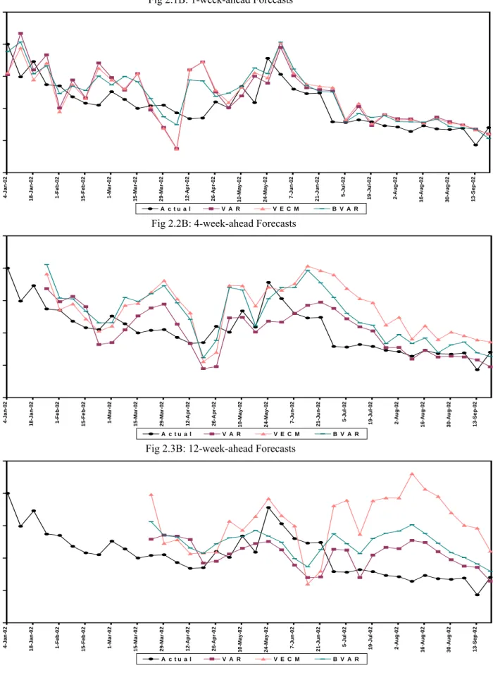
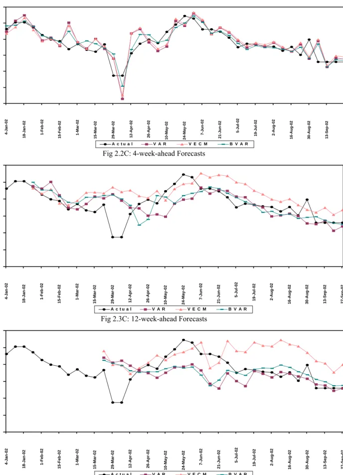
II Call Money Rate

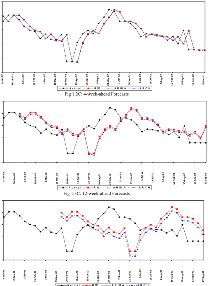
1. Univariate Models

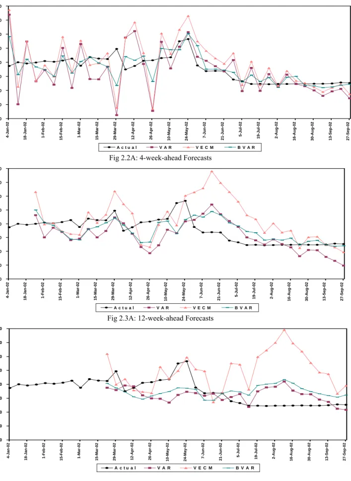
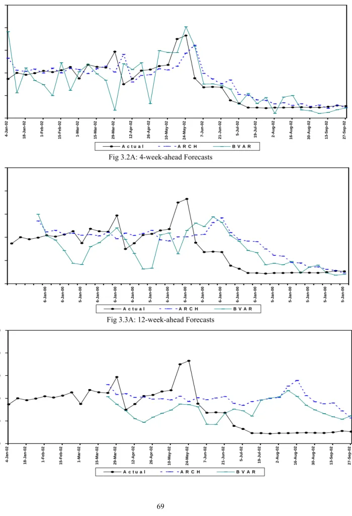
1.1A : 1 Week ahead Forecasts 1.2A : 4 Week ahead Forecasts 1.3A : 12 Week ahead Forecasts

2. Multivariate Models

2.1A : 1 Week ahead Forecasts 2.2A : 4 Week ahead Forecasts 2.3A : 12 Week ahead Forecasts

3. “Best” Univariate Vs. “Best” Multivariate Model

3.1A : 1 Week ahead Forecasts

3.2A : 4 Week ahead Forecasts 3.3A : 12 Week ahead Forecasts 4A : Out of Sample forecasts

(From 25th January to 27th September 2002)

III TB 15-91 – 15-91 Days Treasury Bills

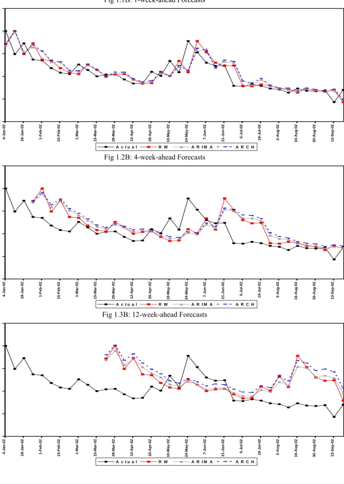
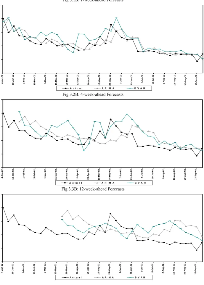
1. Univariate Models:

1.1 B : 1 Week ahead forecasts 1.2 B : 4 Week ahead forecasts 1.3 B : 12 Week ahead forecasts

2. Multivariate Models

2.1 B : 1 Week ahead forecasts 2.2 B : 4 Week ahead forecasts 2.3 B : 12 Week ahead forecasts

3.1 B : 1 Week ahead forecasts 3.2 B : 4 Week ahead forecasts 3.3 B : 12 Week ahead forecasts 4.B : Out of Sample forecasts

(10)

IV G. Sec. 1 – 1 Year Government Securities 1. Univariate Models:

1.1C : 1 Week ahead forecasts 1.2C : 4 Week ahead forecasts 1.3C : 12 Week ahead forecasts

2. Multivariate Models

2.1C : 1 Week ahead forecasts 2.2C : 4 Week ahead forecasts 2.3C : 12 Week ahead forecasts

3.1C : 1 Week ahead forecasts

3.2C : 4 Week ahead forecasts 3.3C : 12 Week ahead forecasts 4C : Out-of-sample forecasts

(from 25th January to 27th September 2002)

V G.Sec. 5 - 5 year Government Securities 1. Univariate Models:

1.1D : 1 Week ahead forecasts 1.2D : 4 Week ahead forecasts 1.3D : 12 Week ahead forecasts

2. Multivariate Models

2.1D : 1 Week ahead forecasts 2.2D : 4 Week ahead forecasts

2.3D : 12 Week ahead forecasts

4.D : Out-of-sample forecasts

(from 25th January to 27th September 2002)

VI G. Sec. 10 – 10 Year Government Securities 1. Univariate Models:

1.1E : 1 Week ahead forecasts 1.2E : 4 Week ahead forecasts 1.3E : 12 Week ahead forecasts

2. Multivariate Models

3. “Best” Univariate Vs. “Best” Multivariate Model

VII Graph 4 (A to E) Out-of-sample forecasts

(11)

Interest Rate Modeling and Forecasting in India

I. Introduction

The interest rate is a key financial variable that affects decisions of consumers, businesses, financial institutions, professional investors and policymakers. Movements in interest rates have important implications for the economy’s business cycle and are crucial to understanding financial developments and changes in economic policy. Timely forecasts of interest rates can therefore provide valuable information to financial market participants and policymakers. Forecasts of interest rates can also help to reduce interest rate risk faced by individuals and firms. Forecasting interest rates is very useful to central banks in assessing the overall impact (including feedback and expectation effects) of its policy changes and taking appropriate corrective action, if necessary.

An important constituent of the package of structural reforms initiated in India in the early 1990s, was the progressive deregulation of interest rates across the broad spectrum of financial markets. As part of this process, the Reserve Bank has taken a number of initiatives in developing financial markets, particularly in the context of ensuring efficient transmission of monetary policy. An important consideration in this regard is the signaling role of monetary policy and its implications for equilibrium interest rates. Furthermore, the evolvement of a ‘multiple indicator approach’ to monetary policy formulation has underscored the information content of rate variables to optimize management goals. Besides, with the progressive integration of financial markets, ‘shocks’ to one market can have quick ‘spill- over’ effects on other markets. In particular, with the liberalization of the external sector, the vicissitudes of capital flows can have implications for the orderly movement of domestic interest rates. Moreover, given the extant large volume of government’s market borrowings and the role of the Reserve Bank in managing the internal debt of the Government, an explicit understanding of the determinants of various interest rates and their expected trajectories over the future could facilitate proper coordination of monetary/interest rate policy, exchange rate policy and fiscal policy.

Against this backdrop, the objective of this study is to develop models to forecast short-term and long-term rates: call money rate, 15-91 days Treasury bill rate and rates on 1-year, 5-years and 10-years government securities. Univariate as well as multivariate models are estimated for each

(12)

models, and ARIMA models with Autoregressive Conditional Heteroscedasticity (ARCH)/Generalised Autoregressive Conditional Heteroscedasiticity (GARCH) effects while multivariate models include Vector Autoregressive (VAR) models specified in levels, Vector Error Correction Models (VECM), and Bayesian Vector Autoregressive (BVAR) models. In the multivariate models, factors such as liquidity, bank rate, repo rate, yield spread, inflation, credit, foreign interest rates and forward premium are considered. The random walk model is used as the benchmark for evaluating the forecast performance of each model.

For each interest rate, a search for the “best” forecasting model, i.e., one that yields the most

accurate forecasts is conducted. This search encompasses the evaluation of the performance of the aforementioned alternative forecasting models. Each model is estimated using weekly data from April 1997 through December 2001 and out-of-sample forecasts up to 36-weeks-ahead are made from January through September 2002. The most significant finding is that multivariate models generally perform better than naive and univariate models and that the forecasting performance of BVAR models is satisfactory for all models.

The format of the study is as follows. Section II highlights, as a backdrop to the ensuing discussion, some stylized facts on interest rates in the context of financial sector reforms and the changes in the monetary policy environment in India. Section III describes the conceptual underpinnings of the different models considered. It also reviews the tests for non-stationarity and describes the methodology for comparing the out-of-sample forecast performance of the models. Section IV presents the empirical results of the alternative models and Section V concludes.

II. Interest Rates and Monetary Policy in India: Some Stylized Facts

The role of interest rates in the monetary policy framework has assumed increasing significance with the initiation of financial sector reforms in the Indian economy in the early 1990s and the progressive liberalisation and integration of financial markets. While the objectives of monetary policy in India have, over the years, primarily been that of maintaining price stability and ensuring adequate availability of credit for productive activities in the economy, the monetary policy environment, instruments and operating procedures have undergone significant changes. It is in this context that the Reserve Bank’s Working Group on Money Supply (1998) observed that the emergence of rate variables in a liberalised environment has adversely impacted upon the predictive stability of the money demand function (although the function continues to exhibit parametric stability) and thus, monetary policy based solely on monetary targets could lack

(13)

precision. The Group also underscored the significance of the interest rate channel of monetary transmission in a deregulated environment. This was, in fact, the underlying principle of the multiple indicator approach that was adopted by the Reserve Bank during 1998-99, whereby a set of economic variables (including interest rates) were to be monitored along with the growth in broad money, for monetary policy purposes. Monetary Policy Statements of the Reserve Bank in recent years have also emphasized the preference for a soft and flexible interest rate environment within the framework of macroeconomic stability.

Interest rates across various financial markets have been progressively rationalized and deregulated during the reform period (See Annexure I for Chronology of Reform Measures in respect of Monetary Policy). The reforms have generally aimed towards the easing of quantitative restrictions, removal of barriers to entry, wider participation, increase in the number of instruments and improvements in trading, clearing and settlement practices as well as informational flows. Besides, the elimination of automatic monetisation of government budget deficit, the progressive reduction in statutory reserve requirements and the shift from direct to indirect instruments of monetary control, have impacted upon the structure of financial markets and the enhanced role of interest rates in the system.

The Reserve Bank influences liquidity and in turn, short-term interest rates, via changes in Cash Reserve Ratio (CRR), open market operations, changes in the Bank Rate, modulating the refinance limits and the Liquidity Adjustment Facility (LAF) [Chart I]. The LAF was introduced in June 2000 to modulate short-term liquidity in the system on a daily basis through repo and reverse repo auctions, and in effect, providing an informal corridor for the call money rate. The LAF sets a corridor for the short-term interest rates consistent with policy objectives. The Reserve Bank also uses the private placement route in combination with open market operations to modulate the market-borrowing programme of the Government. In the post 1997 period, the Bank Rate has emerged as a reference rate as also a signaling mechanism for monetary policy actions while the LAF rate has been effective both as a tool for liquidity management as well as a signal for interest rates in the overnight market.

(14)

Chart I: Determinants of Short-Term Interest Rates in India

CRR: Cash Reserve Ratio (CRR); OMO: Open Market Operations; WMA: Ways and Means Advances; CD: Certificates of Deposits; CP: Commercial Paper.

The liquidity in the system is also influenced by ‘autonomous’ factors like the Ways and Means Advances (WMA) to the Government, developments in the foreign exchange market and stock market and ‘news’.

The changes in the financial sector environment have impacted upon the structure and movement of interest rates during the period under consideration (1997-2002). First, the trends in different interest rates (call money, treasury bill and government securities of residual maturities of one, five and ten years or more) are indicative of a general downward movement particularly from 2000 onwards (Charts II A and B), reflecting the liquidity impact of capital inflows and deft liquidity and debt management in the face of large government borrowings. There were, however, two distinct aberrations in the general trend during this period which essentially reflected the impact of monetary policy and other regulatory actions taken to quell exchange market pressures: the first, which occurred in January 1998 in the wake of the financial crisis in South-East Asia was, in fact, very sharp, while the second occurred around May-August 2000.

CRR Bank

Rate

Liquidity Adjustment Facility (Repo & Reverse Repo)

Reserves Credit Market Determined Rates Refinance OMO

Liquidity

Foreign exchange Market WMA

News and Other Exogenous Factors

Stock Market CPs/CDs

(15)

Chart IIA: Trends in Interest Rates (1997-1998) 0 1 0 2 0 3 0 4 0 5 0 4-Apr -97

2-May-97 _30-May-97 27-Jun-97 25-Jul

-97 22-Aug-97 19-Se p-97 17-Oc t-97 14-Nov-97 12-De c-97 9-Jan-98 6-Fe b-98 6-Mar -98 3-Apr -98

1-May-98 _29-May-98 26-Jun-98 24-Jul

-98 21-Aug-98 18-Se p-98 16-Oc t-98 13-Nov-98 C A L L T B 1 5 - 9 1 G S e c 1 G S e c 5 G S e c 1 0

Chart II B: Trends in Interest Rates (1998-2002)

5.0 7.5 10.0 12.5 15.0 1-Jan-99 26-Fe b-99 23-A p r-99 18-Jun-99 13-A u g-99 8-Oct-99 3-D ec -99 28-Jan-00 _24-Mar -00 19-May-00 14-Jul-00 8-Sep-00 3-N ov-00 29-D ec -00 23-Fe b-01 20-A p r-01 15-Jun-01 10-A u g-01 5-Oct-01 30-N ov-01 25-Jan-02 _22-Mar -02 17-May-02 12-Jul-02 6-Sep-02

(16)

Second, increases in residual maturities have been associated with higher average levels of interest rates (reflecting an upward sloping yield curve) but lower volatility in interest rates (Table 1).

Table 1: Interest Rates – Summary Statistics

(4th Apr 1997-27th Sep 2002)

Interest Rates Mean Max Min Standard

Deviation Call 7.67 45.67 (23rd Jan 1998) 0.18 (4th Apr 1997) 3.46 TB15-91 7.97 ₍₃₀th_{Jan 1998)}21.44 ₍₂₅th_{Apr 1997)}4.49 1.76 Gsec1 9.34 ₍₃₀th_{Jan 1998)}22.86 5.37 (22nd Mar 2002) 1.90 Gsec5 10.14 13.61 (30th Jan 1998) 6.14 (20th Sep 2002) 1.82

Gsec10 10.95 ₍₂₃rd_{Jan 1998)}13.50 ₍₉th_{Aug 2002)}7.38 1.50

Third, there is evidence of progressive financial market integration as reflected in the co-movement of interest rates, particularly from 2000 onwards. The co-co-movement in short-term interest rates is exhibited in Charts III (A and B) and Charts IV (A and B). It may be observed that the co-movement in the call market and the forward premia is particularly pronounced during episodes of excessive volatility in foreign exchange markets. Empirical exercises, as discussed subsequently, also indicate that while the impact of monetary policy changes has been readily transmitted across the shorter end of different markets, their impact on the longer end of the markets has been more limited.

(17)

Chart III A: Trends in Call Rates, Treasury Bill Rates, Repo Rates and Bank Rate (1997-1998)

0 1 0 2 0 3 0 4 0 5 0 4-Apr -97 2- May-97 30- May-97 27- Jun-97 25-Jul -97 22- Aug-97 19-Se p-97 17-Oc t-9 7 14- Nov-97 12-De c-97 9- Jan-9 8 6-Fe b-98 6-Mar -98 3-Apr -98 1- May-98 29- May-98 26- Jun-98 24-Jul -98 21- Aug-98 18-Se p-98 16-Oc t-9 8 13- Nov-98 11-De c-98 C A L L T B 1 5 - 9 1 R e p o B a n k R a t e

Chart III B: Trends in Call Rates, Treasury Bill Rates, Repo Rates and Bank Rate (1999-2002)

4 6 8 10 12 14 16 1-Jan-99

26-Mar-99 18-Jun-99 10-Sep-99 3-Dec-99 25-F

eb-00

19-May-00 11-Aug-00 3-Nov-00 26-Jan-01 20-Apr-01 13-Jul-01 5-Oct-01 28-Dec-01 _22-Mar-02 14-Jun-02 6-Sep-02

(18)

Chart IV A: Trends in Call Rates, Treasury Bill Rates, Government Security (1 year) and Forward Premia (1997-1998) 0 10 20 30 40 50 4-Apr -97 2-May-97

30-May-97 27-Jun-97 25-Jul

-97 22-Aug-97 19-Se p-97 17-Oc t-97 14-Nov-97 12-De c-97 9-Jan-98 6-F eb-98 6-Mar -98 3-Apr -98 1-May-98

29-May-98 26-Jun-98 24-Jul

-98 21-Aug-98 18-Se p-98 16-Oc t-98 13-Nov-98 11-De c-98 C A L L T B 15-91 G Sec 1 fp3

Chart IV B: Trends in Call Rates, Treasury Bill Rates, Government Security (1 year) Rate and Forward Premia (1999-2002)

0 5 1 0 1 5

1-Jan-99

26-Mar-99 18-Jun-99 10-Sep-99 3-Dec-99 25-Feb-00 19-May-00 11-Aug-00 3-Nov-00 26-Jan-01 20-Apr-01 13-Jul-01 5-O

ct-01

28-Dec-01 22-Mar-02 14-Jun-02 6-Sep-02

(19)

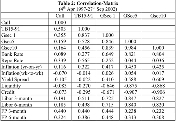
The co-movement between various interest rates could also be gauged by their correlations (Table 2). The correlation between the Bank Rate and other interest rates is found to increase with the length of the maturity period; this is in contrast to the correlations observed in case of the repo rate and, to some extent, the call money rate. The Treasury Bill rate and the rates on Government securities of one, three and ten year maturities, are found to be highly correlated.

Table 2 also reports the correlations between interest rates and a few other variables some of which have been included in the multivariate models discussed subsequently. Expectedly, both liquidity and credit are negatively correlated with interest rates and the magnitude of the correlation increases with the maturity period. In the context of the observed negative correlation between credit and interest rates, it may be added that the notion of 'credit' here refers to credit supply rather than demand. Similarly, the correlation between the year-on-year inflation rate and interest rates is positive and increases with the maturity period of the securities. The yield spread shows a (weak) negative correlation with the call money rate and the Treasury Bill rate, and positive and increasing correlation with interest rates on longer term Government securities. It is also observed that the (positive) correlation of LIBOR rates (both 3-month and 6-month) with domestic interest rates increases with the length of the maturity period in sharp contrast to the correlation between forward premia and domestic interest rates.

Table 2:Correlation-Matrix

(4th_{Apr 1997-27}th_{Sep 2002)}

Call TB15-91 GSec 1 GSec5 Gsec10

Call 1.000 TB15-91 0.503 1.000 Gsec 1 0.355 0.837 1.000 Gsec5 0.159 0.528 0.846 1.000 Gsec10 0.164 0.456 0.839 0.984 1.000 Bank Rate 0.089 0.277 0.649 0.821 0.804 Repo Rate 0.339 0.565 0.252 0.044 0.036 Inflation (yr-on-yr) 0.116 0.322 0.417 0.450 0.425 Inflation(wk-to-wk) -0.070 -0.014 0.026 0.054 0.017 Yield Spread -0.105 -0.022 0.410 0.588 0.609 Liquidity -0.083 -0.270 -0.646 -0.875 -0.868 Credit -0.073 -0.295 -0.671 -0.907 -0.906 Libor 3-month 0.191 0.511 0.725 0.847 0.827 Libor 6-month 0.185 0.498 0.715 0.840 0.820 FP 3-month 0.440 0.440 0.444 0.238 0.232 FP 6-month 0.324 0.386 0.448 0.313 0.308

(20)

III. Alternative Forecasting Models: A Brief Overview

Predicting the interest rate is a difficult task since the forecasts depend on the model used to generate them. Hence, it is important to study the properties of forecasts generated from different models and select the “best” on the basis of an objective criterion. The aim of this study

is to select the “best” model for each interest rate from a number of alternative models estimated1.

The benchmark model for each interest rate is a naïve model that implies that the projection

for the next period is simply the actual value of the variable in the current period. The naïve model is essentially a random walk as described below:

it = it-1 + εt

with E(εt)=0 and E(εtεs)=0 for t≠s.

The one-period-ahead forecast is simply the current value as shown below:

iet+1 = E(it + εt+1) = it

Similarly the k- period-ahead forecast is:

iet+k = it

The next step is to estimate ARIMA models that predict future values of a variable exclusively on the basis of its own past history. These models are then extended to include ARCH/GARCH effects. Clearly, univariate models are not ideal since these do not use information on the relationships between different economic variables. These are, however, a good starting point since predictions from these models can be compared with those from multivariate models.

III.1. ARIMA Models

An ARIMA(p,d,q) can be represented as:

φ (L)(1-L)d yt = δ + θ(L)εt where L = backward shift operator

φ(L) = autoregressive operator = 1-φ1L- φ2L2-………- φpLp

θ(L) = moving average operator = 1- θ1L- θ2L2-…….- θqLq

The stationarity condition for an AR(p) process implies that the roots of φ(L) lie outside the

unit circle, i.e., all the roots of φ(L) are greater than one in absolute value. Restrictions are also

1 _{Fauvel, Paquet and Zimmermann (1999) provide a survey of major methods used to forecast interest rates as well}

as a review of interest rate modelling. Examples of studies that examine forecasting of interest rates are as follows: Ang and Bekaert (1998); Barkoulas and Baum (1997); Bidarkota (1998); Campbell and Shiller (1991); Chiang and Kahl (1991); Cole and Reichenstein (1994); Craine and Havenner.(1988); Deaves (1996); Dua (1988); Froot (1989); Gosnell and Kolb (1997); Gray (1996); Hafer, Hein and MacDonald (1992); Holden and Thompson (1996); Iyer and Andrews (1999); Jondeau and Sedillot (1999); Jorion and Mishkin (1991); Kolb and Stekler (1996); Park and Switzer (1997); Pesando (1981); Prell (1973); Roley (1982); Sola and Driffil (1994); and Throop (1981).

(21)

imposed on θ(L) to ensure invertibility so that the MA(q) part can be written in terms of an infinite autoregression on y. Furthermore, if a series requires differencing ‘d’ times to yield a stationary series, then the differenced series is modelled as an ARMA(p,q) process or equivalently, an ARIMA(p,d,q) model is fitted to the series.

Other criteria employed to select the best-fit model include parameter significance, residual diagnostics, and minimization of the Akaike Information Criterion and the Schwartz Bayesian Criterion.

ARIMA-ARCH/GARCH Models

The assumption of constant variance of the innovation process in the ARIMA model can be relaxed following Engle’s (1982) seminal paper and its extension by Bollerslev (1986) on modelling the conditional variance of the error process. One possibility is to model the conditional variance as an AR(q) process using the square of the estimated residuals, i.e., the autoregressive conditional heteroscedasticity (ARCH) model. The conditional variance thus follows an MA process, while in its generalized version – GARCH – it follows an ARMA process. Adding this information can improve the performance of the ARIMA model due to the presence of the volatility clustering effect

characteristic of financial series. In other words, the errors, εt although serially uncorrelated

through the white noise assumption, are not independent since they are related through their

second moments. Hence, large values of εt are likely to be followed by large values of εt+1 of

either sign. Consequently, a realisation of εt exhibits behaviour in which clusters of large

observations are followed by clusters of small ones.

According to Engle's basic ARCH model, the conditional variance of the shock that occurs at time t is a linear function of the squares of the past shocks. For example, an ARCH(1) model is specified as:

Yt = E [Yt | Ωt-1] + εt

εt = vt√ ht and ht = α0 + α1ε2t-1

where vt is a white noise process and is independent of εt-1 and εt has mean of zero and is

uncorrelated. For the conditional variance ht to be non-negative, the conditions α0 > 0 and α1≥

0 and 0 ≤ α1 ≤ 1 (for covariance stationarity) must be satisfied. To understand why the ARCH

model can describe volatility clustering, observe that the above equations show that the

(22)

onditional variance of εt is an increasing function of the shock that occurred in the previous

time periods. Therefore if εt-1 is large (in absolute value), εt is expected to be large (in absolute

value) as well. In other words, large (small) shocks tend to be followed by large (small) shocks, of either sign.

To model extended persistence, generalizations of the ARCH(1) model such as including

additional lagged squared shocks can be considered as in the ARCH (q) model below:

ht = α0 + α1ε2t-1+α2ε2t-2+…..+αqε2t-q

For non-negativeness of the conditional variance, the following conditions must be met:

α0 > 0, α1 >0 and 1 > Σiαi ≥ 0 for all i = 1,2,3, ……, q.

To capture the dynamic patterns in conditional volatility adequately by means of an ARCH (q) model, q often needs to be quite large. Estimating the parameters in such a model can therefore be cumbersome because of stationarity and non-negativity constraints. However, adding lagged conditional variances to the ARCH model can circumvent this drawback. For

example, including ht-1 to the ARCH (1) model, results in the Generalized ARCH (GARCH)

model of the order (1,1):

ht = α0 + α1ε2t-1+ β1ht-1

The parameters in this model should satisfy α0 > 0, α1 >0 and β1 ≥ 0 to guarantee that ht

≥0, while α1 must be strictly positive for to β1 be identified. Generalising, the GARCH (p,q)

model is given by:

ht = α0 + ti q i i − =

∑

2 1

ε

α

₊ p _t_i i i

h

− =

∑

1

β

ht = α0 + α(L) ε2t + β(L) ht

Assuming that all the roots of 1 - β(L) are outside the unit circle, the model can be

rewritten as an infinite-order ARCH model.

As indicated above, univariate models such as ARIMA and ARCH/GARCH models utilize information only on the past values of the variable to make forecasts. We now consider multivariate forecasting models that rely on the interrelationships between different variables.

III.2 VAR and BVAR Modelling

As a prelude to the discussion on multivariate models, it is apposite to note that according to the Statement on Monetary and Credit Policy for 2002-03, short-term forecasts of interest rates need to

(23)

take cognizance of possible movements in all other macreconomic variables including investment, output and inflation, which are, in turn, susceptible to unanticipated changes emanating from unforseen domestic or international developments. Multivariate forecasting models address such concerns and are often formulated as simultaneous equations structural models. In these models, economic theory not only dictates what variables to include in the model, but also postulates which explanatory variables to use to explain any given independent variable. This can, however, be problematic when economic theory is ambiguous. Further, structural models are generally poorly suited for forecasting. This is because projections of the exogenous variables are required to forecast

the endogenous variablesAnother problem in such modelsis that proper identification of individual

equations in the system requires the correct number of excluded variables from an equation in the model.

A vector autoregressive (VAR) model offers an alternative approach, particularly useful for forecasting purposes. This method is multivariate and does not require specification of the projected values of the exogenous variables. Economic theory is used only to determine the variables to include in the model.

Although the approach is "a theoretical," a VAR model approximates the reduced form of a structural system of simultaneous equations. As shown by Zellner (1979), and Zellner and Palm (1974), any linear structural model theoretically reduces to a VAR moving average (VARMA) model, whose coefficients combine the structural coefficients. Under some conditions, a VARMA model can be expressed as a VAR model and as a Vector Moving Average (VMA) model. A VAR model can also approximate the reduced form of a simultaneous structural model. Thus, a VAR model does not totally differ from a large-scale structural model. Rather, given the correct restrictions on the parameters of the VAR model, they reflect mirror images of each other.

The VAR technique uses regularities in the historical data on the forecasted variables. Economic theory only selects the economic variables to include in the model. An unrestricted VAR model (Sims 1980) is written as follows:

yt = C + A(L)yt +et, where

y = an (nx1) vector of variables being forecast;

A(L) = an (nxn) polynomial matrix in the back-shift operator L with lag length p,

= A1L + A2L2 +...+ApLp;

(24)

e = an (nx1) vector of white noise error terms.

The model uses the same lag length for all variables. One serious drawback exists -- overparameterization produces multicollinearity and loss of degrees of freedom that can lead to inefficient estimates and large out-of-sample forecasting errors. One solution excludes insignificant variables/lags based on statistical tests.

An alternative approach to overcome overparameterization uses a Bayesian VAR model as described in Litterman (1981), Doan, Litterman and Sims (1984), Todd (1984), Litterman (1986), and Spencer (1993). Instead of eliminating longer lags and/or less important variables, the Bayesian technique imposes restrictions on these coefficients on the assumption that these are more likely to be near zero than the coefficients on shorter lags and/or more important variables. If, however, strong effects do occur from longer lags and/or less important variables, the data can override this assumption. Thus the Bayesian model imposes prior beliefs on the relationships between different variables as well as between own lags of a particular variable. If these beliefs (restrictions) are appropriate, the forecasting ability of the model should improve. The Bayesian approach to forecasting therefore provides a scientific way of imposing prior or judgmental beliefs on a statistical model. Several prior beliefs can be imposed so that the set of beliefs that produces the best forecasts is selected for making forecasts. The selection of the Bayesian prior, of course, depends on the expertise of the forecaster.

The restrictions on the coefficients specify normal prior distributions with means zero and small standard deviations for all coefficients with decreasing standard deviations on increasing lags, except for the coefficient on the first own lag of a variable that is given a mean of unity. This so-called "Minnesota prior" was developed at the Federal Reserve Bank of Minneapolis and the University of Minnesota.

The standard deviation of the prior distribution for lag m of variable j in equation i for all

i, j, and m -- S(i, j, m) -- is specified as follows:

S(i, j, m) _{= {wg(m)f(i, j)}si/sj;}

f(i, j) = 1, if i = j;

= k otherwise (0 < k < 1); and

g(m) = m-d, d > 0.

The term _si equals the standard error of a univariate autoregression for variable i. The

(25)

specification of the prior without consideration of the magnitudes of the variables. The parameter w measures the standard deviation on the first own lag and describes the overall

tightness of the prior. The tightness on lag m relative to lag 1 equals the function g(m), assumed

to have a harmonic shape with decay factor d. The tightness of variable j relative to variable i in

equation i equals the function f(i, j).

To illustrate, assume the following hyperparameters: w = 0.2; d = 2.0; and f(i, j) = 0.5.

When w = 0.2, the standard deviation of the first own lag in each equation is 0.2, since g(1) = f(i,

j) = si/sj = 1.0. The standard deviation of all other lags equals _{0.2[si/sj{g(m)f(i, j)}].} For m = 1,

2, 3, 4, and d = 2.0, g(m) = 1.0, 0.25, 0.11, 0.06, respectively, showing the decreasing influence

of longer lags. The value of f(i, j) determines the importance of variable j relative to variable i in

the equation for variable i, higher values implying greater interaction. For instance, f(i, j) = 0.5

implies that relative to variable i, variable j has a weight of 50 percent. A tighter prior occurs by

decreasing w, increasing d, and/or decreasing k. Examples of selection of hyperparameters are

given in Dua and Ray (1995), Dua and Smyth (1995), Dua and Miller (1996) and Dua, Miller and Smyth (1999).

The BVAR method uses Theil's (1971) mixed estimation technique that supplements data with prior information on the distributions of the coefficients. With each restriction, the number of observations and degrees of freedom artificially increase by one. Thus, the loss of degrees of freedom due to overparameterization does not affect the BVAR model as severely.

Another advantage of the BVAR model is that empirical evidence on comparative out-of-sample forecasting performance generally shows that the BVAR model outperforms the unrestricted VAR model. A few examples are Holden and Broomhead (1990), Artis and Zhang (1990), Dua and Ray (1995), Dua and Miller (1996), Dua, Miller and Smyth (1999).

The above description of the VAR and BVAR models assumes that the variables are stationary. If the variables are nonstationary, they can continue to be specified in levels in a BVAR model because as pointed out by Sims et. al (1990, p.136) ‘……the Bayesian approach is entirely based on the likelihood function, which has the same Gaussian shape regardless of the presence of nonstationarity, [hence] Bayesian inference need take no special account of nonstationarity’. Furthermore, Dua and Ray (1995) show that the Minnesota prior is appropriate even when the variables are cointegrated.

(26)

In the case of a VAR, Sims (1980) and others, e.g. Doan (1992), recommend estimating the VAR in levels even if the variables contain a unit root. The argument against differencing is that it discards information relating to comovements between the variables such as cointegrating relationships. The standard practice in the presence of a cointegrating relationship between the variables in a VAR is to estimate the VAR in levels or to estimate its error correction representation, the vector error correction model, VECM. If the variables are nonstationary but not cointegrated, the VAR can be estimated in first differences.

The possibility of a cointegrating relationship between the variables is tested using the Johansen and Juselius (1990) methodology as follows.

Consider the p-dimensional vector autoregressive model with Gaussian errors t t p t p t t A y A y D A y = ₁ ₋₁+...+ ₋ +Ψ. + ₀ +ε

where y_t is an m×1 vector of I(1) jointly determined variables, D is a vector of deterministic or

nonstochastic variables, such as seasonal dummies or time trend. The Johansen test assumes that

the variables in y_t are I(1). For testing the hypothesis of cointegration the model is

reformulated in the vector error-correction form t t p i i t i t t y y A D y =−Π + Γ∆ + +Ψ +ε ∆

∑

− = − − 0 1 1 1 where

Here the rank of Π is equal to the number of independent cointegrating vectors. Thus, if

the rank(Π)=0, then the above model will be the usual VAR model in first differences.

Similarly, if the vector yt is I(0), i.e., if all the variables are stationary, then all characteristic

roots will be greater than unity and hence Π will be a full rank m x m matrix. If the elements of

vector yt are I(1) and cointegrated with rank (Π)=r, then Π =αβ′, where α and β are m x r full

column rank matrices and there are r < m linear combinations of yt. The model can easily be

extended to include a vector of exogenous I(1) variables.

∑

+ = = − = − = Γ − = Π p i j j i p i i m A A i p I 1 1 . 1 ,..., 1 , ,

(27)

Suppose the m characteristic roots of Π are λ1, λ2, λ3…λm. If the variables in yt are not

cointegrated, the rank of Π is zero and all these characteristic roots will be equal zero. Since ln

(1)=0, ln (1-λi) will be equal to zero if the variables are not cointegrated. Similarly, if the rank

of Π is unity, then if 0 < λ1 <1 so that ln(1-λ1) will be negative and λi=0 (∀i g1) so that ln

(1-λi) =0 (∀i g1).

λtrace and λmax tests can be used to test for the number of characteristic roots that are

significantly different from unity.

( )

∑

+ = ∧ ⎟ ⎠ ⎞ ⎜ ⎝ ⎛ − − = n r i i trace r T 1 1 ln λ λ

(

)

⎟ ⎠ ⎞ ⎜ ⎝ ⎛ − − = + ∧₊₁ max r,r 1 Tln 1 λr λ

where λ∧_i= the estimated values of the characteristic roots of Π

T = the number of usable observations

λtrace tests the null hypothesis that the number of distinct cointegrating vectors is less than or

equal to r against a general alternative. If λi=0 for all i, then λtrace equals zero. The further the

estimated characteristic roots are from zero, the more negative is ln(1-λi) and the larger the λtrace

statistic. λmax tests the null that the number of cointegrating vectors is r against the alternative of

r+1 cointegrating vectors. If the estimated characteristic root is close to zero, λmax will be small.

Since λmax test has sharper alternative hypothesis, it is used to select the number of cointegrating

vectors in this study.

Under cointegration, the VECM can be represented as t t t p i i t t y y A D y =−αβ + Γ∆ + +Ψ +ε ∆ − ₋ = −

∑

1 0 1 1 1 '

where α is the matrix of adjustment coefficients. If there are non-zero cointegrating vectors, then

some of the elements of α must also be non zero to keep the elements of yt from diverging from

equilibrium.

The concept of Granger causality can also be tested in the VECM framework. For example, if two variables are cointegrated, i.e. they have a common stochastic trend, causality in the Granger (temporal) sense must exist in at least one direction (Granger, 1986; 1988). Since

(28)

Granger causality is also a test of whether one variable can improve the forecasting performance of another, it is important to test for it to evaluate the predictive ability of a model.

In a two variable VAR model, assuming the variables to be stationary, we say that the first variable does not Granger cause the second if the lags of the first variable in the VAR are jointly not significantly different from zero. This concept is extended in the framework of a VECM to include the error correction term in addition to lagged variables of the variables. Granger-causality can then be tested by (i) the statistical significance of the lagged error correction term by a standard t-test; and (ii) a joint test applied to the significance of the sum of

the lags of each explanatory variables, by a joint F or Wald χ2_{test. Alternatively, a joint test of}

all the set of terms described in (i) and (ii) can be conducted by a joint F or a Wald χ2_{test. The}

third option is used in this paper.

III.3 Testing for Nonstationarity

Before estimating any of the above models, the first econometric step is to test if the series are nonstationary or contain a unit root. Several tests have been developed to test for the presence of a unit root. In this study, we focus on the augmented Dickey-Fuller (1979, 1981) test, the Phillips Perron (1988) test and the KPSS test proposed by Kwiatkowski et al. (1992).

To test if a sequence yt contains a unit root, three different regression equations are

considered. p ∆yt= α + γyt-1 + θt + ∑βi∆yt-i+1 + εt (1) i=2 p ∆yt= α + γyt-1 + ∑βi∆yt-i+1 + εt (2) i=2 p ∆yt= γyt-1 + ∑βi∆yt-i+1 + εt (3) i=2

The first equation includes both a drift term and a deterministic trend; the second excludes the deterministic trend; and the third does not contain an intercept or a trend term. In all three

equations, the parameter of interest is γ. If γ=0, the yt sequence has a unit root. The estimated

t-statistic is compared with the appropriate critical value in the Dickey-Fuller tables to determine

if the null hypothesis is valid. The critical values are denoted by ττ, τµ and τ for equations (1),

(29)

FollowingDoldado, Jenkinson and Sosvilla-Rivero (1990), a sequential procedure is used to test for the presence of a unit root when the form of the data-generating process is unknown. Such a procedure is necessary since including the intercept and trend term reduces the degrees of freedom and the power of the test implying that we may conclude that a unit root is present when, in fact, this is not true. Further, additional regressors increase the absolute value of the critical value making it harder to reject the null hypothesis. On the other hand, inappropriately omitting the deterministic terms can cause the power of the test to go to zero (Campbell and Perron, 1991).

The sequential procedure involves testing the most general model first (equation 1). Since the power of the test is low, if we reject the null hypothesis, we stop at this stage and conclude that there is no unit root. If we do not reject the null hypothesis, we proceed to determine if the trend term is significant under the null of a unit root. If the trend is significant, we retest for the presence of a unit root using the standardised normal distribution. If the null of a unit root is not rejected, we conclude that the series contains a unit root. Otherwise, it does not. If the trend is not significant, we estimate equation (2) and test for the presence of a unit root. If the null of a unit root is rejected, we conclude that there is no unit root and stop at this point. If the null is not rejected, we test for the significance of the drift term in the presence of a unit root. If the drift term is significant, we test for a unit root using the standardised normal distribution. If the drift is not significant, we estimate equation (3) and test for a unit root.

We also conduct the Phillips-Perron (1988) test for a unit root. This is because the Dickey-Fuller tests require that the error term be serially uncorrelated and homogeneous while the Phillips-Perron test is valid even if the disturbances are serially correlated and heterogeneous. The test statistics for the Phillips-Perron test are modifications of the t-statistics employed for the Dickey-Fuller tests but the critical values are precisely those used for the Dickey-Fuller tests. In general, PP test is preferred to the ADF tests if the diagnostic statistics from the ADF regressions indicate autocorrelation or heteroscedasticity in the error terms. Phillips and Perron (1988) also show that when the disturbance term has a positive moving average component, the power of the ADF tests is low compared to the Phillips-Perron statistics so that the latter is preferred. If, however, a negative moving average term is present in the error term, the PP test tends to reject the null of a unit root and, therefore, ADF tests are preferred.

(30)

In both the ADF and the PP test, the unit root is the null hypothesis. A problem with classical hypothesis testing is that it ensures that the null hypothesis is not rejected unless there is strong evidence against it. Therefore these tests tend to have low power, that is, these tests will often indicate that a series contains a unit root. Kwiatkowski et al. (1992), therefore, suggest that, based on classical methods, it may be useful to perform tests of the null hypothesis of stationarity in addition to tests of the null hypothesis of a unit root. Tests based on stationarity as the null can then be used for confirmatory analysis, that is, to confirm conclusions about unit roots. Of course, if tests with stationarity as the null as well as tests with unit root as the null, both reject or fail to reject the respective nulls, there is no confirmation of stationarity or nonstationarity.

KPSS test with the null hypothesis of difference stationarity

To test for difference stationarity (DS), KPSS assume that the series yt with T observations

(t=1,2,…,T) can be decomposed into the sum of a deterministic trend, random walk and stationary error:

yt = δt + rt + εt

where rt is a random walk

rt = rt-1 + µt

and µt is independently and identically distributed with mean zero and variance σ2µ. The

initial value r0 is fixed and serves the role of an intercept. The stationarity hypothesis is

σ2

µ=0. If we set δ = 0, then under the null hypothesis yt is stationary around a level (r0).

Let the residuals from the regression of yt on an intercept be et, t=1,2,…,T. The

partial sum process of the residuals is defined as:

t

St = Σ et.

i=1

The long run variance of the partial error process is defined by KPSS as

σ2_{= limT}-1_E(S2

T).

T→∝

A consistent estimator of σ2_{, s}2₍_l_{), can be constructed from the residuals e}

t as

T l T

s2(l) = T-1∑ e2t + 2T-1∑ w(s,l) ∑ etet-s

t=1 s=1 t=s+1

where w(s,l) is an optional lag window that corresponds to the selection of a spectral window. KPSS

(31)

non-negativity of s2(l). The lag operator l corrects for residual serial correlation. If the residual series are

independently and identically distributed, a choice of l = 0 is appropriate.

The test statistic for the DS null hypothesis is

∧ T

ηµ = T-2∑ S2t/s2(l). t=1

∧

KPSS report the critical values of ηµ (p. 166) for the upper tail test.

Thus, three tests, augmented Dickey-Fuller, Phillips Perron and KPSS tests, are used to test for the presence of a unit root. The KPSS test, with the null of stationarity, helps to resolve conflicts between ADF and PP tests. If two of these three tests indicate nonstationarity for any series, we conclude that the series has a unit root.

In sum, the study proceeds as follows. First, the series are tested for the presence of a unit root using the augmented Dickey-Fuller, Phillips Perron and KPSS tests. If the interest rate series are nonstationary, univariate models, i.e. ARIMA without and with ARCH-GARCH effects, are fitted to differenced, stationary series.

Multivariate models include VAR, VECM, and BVAR models. To estimate VAR models, if all the variables are nonstationary and integrated of the same order, the Johansen test is conducted for the presence of cointegration. If a cointegrating relationship exists, the VAR model can be estimated in levels. Tests for Granger causality are also conducted in the VECM framework to evaluate the forecasting ability of the model. Lastly, Bayesian vector autoregressive models are estimated that impose prior beliefs on the relationships between different variables as well as between own lags of a particular variable. If these beliefs (restrictions) are appropriate, the forecasting ability of the model should improve.

The forecasting ability of each model is evaluated by examining the performance of out-of-sample forecasts and the “best” forecasting model is selected.

III.4 Evaluation of Forecasting Models

The “best” forecasting model is one that produces the most accurate forecasts. This means that the predicted levels should be close to the actual realized values. Furthermore, the predicted variables should move in the same direction as the actual series. In other words, if a series is rising (falling), the forecasts should reflect the same direction of change. If a series is changing direction, the forecasts should identify this.

(32)

To select the best model, the alternative models are initially estimated using weekly data over the period April 1997 to December 2001 and tested for out-of-sample forecast accuracy from January 2002 to September 2002. In other words, by continuously updating and reestimating, we conduct a real world forecasting exercise to see how the models perform. The model that produces the most accurate one- through thirty-six-week-ahead forecasts is designated the “best” model for a particular interest rate.

To test for accuracy, the Theil coefficient (Theil, 1966), is used that implicitly incorporates

the naïve forecasts as the benchmark. If A_t+n denotes the actual value of a variable in period (t+n),

and _tF_t+n the forecast made in period t for (t+n), then for T observations, the Theil U-statistic is

defined as follows:

U = [Σ(A_t+n_-_tF_t+n)2/Σ(A_t+n - A_t)2]0.5.

The U-statistic measures the ratio of the root mean square error (RMSE) of the model

forecasts to the RMSE of naive, no-change forecasts (forecasts such that _tF_t+n= A_t). The RMSE

is given by the following formula:

RMSE = [Σ(A_t+n_-_tF_t+n)2/T]0.5.

A comparison with the naïve model is, therefore, implicit in the U-statistic. A U-statistic of 1 indicates that the model forecasts match the performance of naïve, no-change forecasts. A

U-statistic >1 shows that the naïve forecasts outperform the model forecasts. If U is < 1, the

forecasts from the model outperform the naïve forecasts. The U-statistic is, therefore, a relative measure of accuracy and is unit-free.

Since the U-statistic is a relative measure, it is affected by the accuracy of the naïve

forecasts. Extremely inaccurate naïve forecasts can yield U <1, falsely implying that the model

forecasts are accurate. This problem is especially applicable to series with trend. The RMSE, therefore, provides a check on the U-statistic and is also reported.

To evaluate the forecast performance, the models are continually updated and reestimated. The models are estimated for the initial period April 1997 through December 2001. Forecasts for up to 36-weeks-ahead are computed. One more observation is added to the sample and forecasts up to 36-weeks-ahead are again generated, and so on. Based on the out-of-sample forecasts for the period January through September 2002, the Theil U-statistics and RMSE are computed for one- to 36-weeks-ahead forecasts and the average of successive four U-statistics

(33)

and RMSE are also computed. The overall average of the U statistic and the RMSE for up to 36-weeks-ahead forecasts is also calculated to gauge the accuracy of a model.

IV. Estimation of Alternative Forecasting Models

IV.1 Tests for Nonstationarity

The first step in the estimation of the alternative models is to test for nonstationarity. Three alternative tests are used, i.e., the augmented Dickey-Fuller (ADF) test, Phillips Perron (PP) test and the KPSS test. If there is a conflict between the ADF and PP tests, this is resolved using the KPSS test. If at least two of the three tests show the existence of a unit root, the series is considered as nonstationary. The tests for nonstationarity are reported using weekly data from April 1997 to September 2002. Unit root tests are also conducted for a longer time span using monthly data from early 1990s onwards since Shiller and Perron (1985) and Perron (1989) note that when testing for unit roots, the total span of the time period is more important than the frequency of observations. In the same vein, Hakkio and Rush (1991) show that cointegration is a long-run concept and hence requires long spans of data rather than more frequently sampled observations to yield tests for cointegration with higher power. Since the inferences from monthly data conform to those from weekly data, the monthly results are not reported.

Table 1.1A reports the augmented Dickey-Fuller and Phillips Perron tests for the five interest rates under study – call money rate, 15-91 days Treasury Bill rate, and 1-, 5-, and 10-year government securities (residual maturity). Table 1.1B reports the same tests for variables used in multivariate models while Table 1.2 gives the results of the KPSS test for all the variables used in this study. The results of these three tests are summarised in Table 1.3 and show that except for the week-to-week inflation rate, all the variables can be treated as nonstationary. Testing for differences of each variable confirms that all the variables are integrated of order one.

IV.2 Estimation of Univariate and Multivariate Models

The univariate best-fit models (Tables 2A-2E) for the first-differenced interest rates are estimated as follows for the period April 1997 to December 2002:

Call money rate: ARMA (2,2); ARMA(2,2)-GARCH(1,1)

Treasury Bill rate – 15-91 days ARMA(3,0); ARMA(3,0)-ARCH(1)

(34)

Government Securities – 5-years ARMA(2,0); ARMA(2,0)-ARCH(2) Government Securities – 10-years ARMA(1,0); ARMA(1,0)-ARCH(1)

These models are reported in Tables 2A-2E and are used to generate out-of-sample forecasts from January through September 2002.

Three kinds of multivariate models are estimated – vector autoregressive (VAR) models, vector error correction models (VECM), and Bayesian vector autoregressive (BVAR) models. First, a VAR model is estimated. Second, its error correction representation is derived. Finally, alternative BVAR models are estimated using the optimal lag length determined for an unrestricted VAR.

To estimate a VAR, it is important to first determine if the variables included in a VAR are also cointegrated. If the variables are indeed cointegrated, the VAR model can be estimated in level-form. Accordingly, we first test for cointegration between the variables for each of the interest rates. The optimal lag length for each VAR system is determined by the Akaike Information Criterion, Schwartz Bayesian Criterion and the likelihood ratio test.

Selection of Variables

To estimate the multivariate models, the variables are selected for each model on the basis of economic theory and out-of-sample forecast accuracy. Several factors can impact interest rates. Furthermore, their impacts may differ depending upon the maturity spectrum of the interest rates. For instance, for short-term/medium-term rates, factors that might impact interest rates include monetary policy; liquidity, demand and supply of credit, actual and expected inflation, external factors such as foreign interest rates and change in foreign exchange reserves, and the level of economic activity. For long-term interest rates, demand and supply of funds and expectations about government policy might be relatively more important.

Some of these factors also emerge from the stylized model developed by Dua and Pandit (2002) under covered interest parity condition. The equation for the real interest rate derived from their model can be expressed as a function of expected inflation, foreign interest rate, forward premium, and variables to denote fiscal and monetary effects. Based on this model, the inflation rate, foreign interest rate, forward premium and a variable to gauge monetary policy are included in the forecasting model. In addition to these variables, the following are also included: yield spread (discussed below); liquidity in the m