Prediction and Modelling of Complex Social
Networks and Their Evolution
by
Akanda Wahid -Ul- Ashraf
A thesis submitted in partial fulfilment for the degree of Doctor of Philosophy
in the
Department of Computing and Informatics
I, Akanda Wahid -Ul- Ashraf, declare that this thesis titled, ‘Adaptive and robust approach for predictive modelling of dynamics and evolution of Complex Social Networks’ and the work presented in it are my own. I confirm that:
This work was done wholly or mainly while in candidature for a research degree at this
University.
Where any part of this thesis has previously been submitted for a degree or any other
qualification at this University or any other institution, this has been clearly stated.
Where I have consulted the published work of others, this is always clearly attributed. Where I have quoted from the work of others, the source is always given. With the
excep-tion of such quotaexcep-tions, this thesis is entirely my own work.
I have acknowledged all main sources of help.
Where the thesis is based on work done by myself jointly with others, I have made clear
exactly what was done by others and what I have contributed myself.
Signed:
Date:
find out what they are about. That’s the science part.”
Abstract
Department of Computing and Informatics
Doctor of Philosophy
byAkanda Wahid -Ul- Ashraf
This thesis focuses on complex social networks in the context of computational approaches for their prediction and modelling. The increasing popularity and advancement of social net-works paired with the availability of social network data enable empirical analysis, inference, prediction and modelling of social patterns. This data-driven approach towards social science is continuously evolving and is crucial for modelling and understanding of human social be-haviour including predicting future social interactions for a wide range of applications. The main difference between traditional datasets and network datasets is the presence of the rela-tional components (links) between instances (nodes) of the network. These links and nodes induce intricate local and global patterns, defining the topology of a network. The topology is ever evolving, determining the dynamics of such a networked system. The work presented in this thesis starts with an extensive analysis of three standard network models, in terms of their properties and self-interactions as well as the size and density of the resultant graphs. These crucial analysis and understanding of the main network models are utilised to later develop a comprehensive network simulation framework. A set of novel nature-inspired link prediction approaches are then developed to predict the evolution of networks, based solely on their topolo-gies. Building on top of these approaches, enhanced topological representations of networks are subsequently combined with node characteristics for the purpose of node classification. Finally, the proposed classification methods are extensively evaluated using simulated networks from our network simulation framework as well as two real-world citation networks. The link prediction approaches proposed in this research show that the topology of the network can be further ex-ploited to improve the prediction of future relationships. Moreover, this research demonstrates the potential of blending state-of-the-art Machine Learning techniques with graph theory. To accelerate such advancements in the field of network science, this research also offers an open-source software to provide high-quality synthetic datasets.
I would like to give thanks to my parents and my younger brother, Talha, for their help, inspira-tion, and support for all the achievements in my life.
I would like to express my gratitude towards both of my supervisors, Prof Marcin Budka and Prof Katarzyna Musial for supporting and guiding me throughout my research. It has been an amazing experience to be able to work under their supervisions, which has made me more organised and increased my research skills.
I also would like to thank Bournemouth University (BU) for providing me with a PhD stu-dentship, which has made this work possible.
I would like to thank all the staffs at Bournemouth University for creating such a friendly and excellent research environment. Especially I would like to thank all the Research Administrators and the Doctoral College for their immense help and support towards the graduate students. I also would like to thank all my colleagues at Bournemouth University, especially in my lab for creating such a friendly environment, which has facilitated an outstanding work environment. I would like to thank my friend and colleague Dr Rashid Bakirov with whom I have played a lot of table-football, which has been a good source of fun in our lab. I would also like to thank Dr Arif Reza Anwary who has been an inspiration for me.
A special thanks towards my friend Gareth Leaney for helping me with academic writing at the beginning of my journey towards this PhD.
A very special thanks to my very dear friend Dr Saad Mohamad, who deserves a separate para-graph, for giving me company during most of my time at BU.
I would like to thank my Grandmother, Fatema Kabir for her tremendous support towards my academic journey. I would also like to thank my cousins, Mehnaz Hoque and Mohammad Moshiul Hoque Riad for their never-ending support and friendship at any given point in my life. I would like to show my gratitude towards two of my best friends, Aubdullah Munim and Sabbir Ahamed for their friendship and support which has encouraged me towards some of the biggest achievements in my life.
Finally, a special thanks to Sue Burt, Sharon Hartwell, and Tim Peters from the BU chaplaincy team for their immense help and support during my entire journey of this thesis at Bournemouth University.
Declaration of Authorship i
Abstract iii
Acknowledgements iv
List of Figures viii
List of Tables xi
1 Introduction 1
1.1 Link Prediction . . . 4
1.2 Missing Links and Node Classification . . . 5
1.3 Social Network Simulation . . . 6
1.4 Original Contributions and Outputs. . . 8
1.4.1 Research Contribution . . . 8 1.5 Thesis Structure . . . 10 2 Literature Review 12 2.1 Properties of Networks . . . 12 2.1.1 Centrality . . . 14 2.2 Mesoscale Structures . . . 17 2.2.1 Communities . . . 17 2.2.2 Core-periphery . . . 17 2.3 Link Prediction . . . 18
2.3.1 Physics-inspired Approaches for Link Prediction in Social Networks. . 18
2.3.2 Newton’s Gravity in Social Sciences . . . 19
2.3.3 Link Prediction Methods Classifications . . . 20
2.3.4 Link Prediction Methods . . . 22
2.3.5 Network Models . . . 26
2.4 GCN - A Neural Network Model for Graphs . . . 29
3 Methodology 30 3.1 Problem Statement and Research Questions . . . 30
3.2 Objectives . . . 32
3.3 Tasks . . . 33
4 Overview of Network Models - Simulation Study 35
4.1 A Brief Overview of Network Generators Landscape . . . 36
4.2 Proposed NetSim Framework . . . 37
4.2.1 Network Models . . . 37
4.2.2 Network Generation Approach. . . 38
4.3 Design of the Experiment . . . 39
4.4 Results and Analysis . . . 41
4.4.1 Number of Edges and Vertices . . . 41
4.4.2 Closeness Centrality . . . 42
4.4.3 Betweeness Centrality . . . 43
4.4.4 Average Shortest Path . . . 44
4.4.5 Global Clustering Coefficient . . . 46
4.4.6 Discussion . . . 48
4.5 Chapter Summary . . . 48
5 Newton’s Law of Universal Gravitation in Link Prediction 50 5.1 Experimental Setup . . . 52
5.1.1 Datasets . . . 54
5.1.2 Data Partition . . . 57
5.2 Experimental Setup . . . 57
5.3 Results. . . 58
5.3.1 Overall performance using AUC . . . 61
5.3.1.1 Combinations with Katz . . . 63
5.3.1.2 Combinations with AdamicAdar (AA) . . . 63
5.3.1.3 Combinations with Common Neighbours (CN). . . 64
5.3.1.4 Combinations with Jaccard’s Coefficient (JC) . . . 64
5.3.1.5 Combinations with Average Commute Time (ACT) . . . 65
5.3.1.6 Combinations with Average Commute Time Normalised (ACTN) 66 5.3.1.7 Combinations with Rooted PageRank (RPR) . . . 66
5.3.1.8 Combinations with Pseudoinverse of the Laplacian matrix (PsIn-Lap) . . . 67
5.3.1.9 Combinations with Local Path Index (LPI) . . . 67
5.3.1.10 Combinations with Leicht-Holme-Newman Global Index (LGI) 68 5.3.1.11 Combinations with Matrix Forest Index (MFI) . . . 68
5.3.1.12 Combinations with Shortest Path . . . 69
5.3.2 Best Methods . . . 70
5.3.3 Results Analysis for each Dataset . . . 71
5.3.4 Computational Complexity . . . 74
5.4 Results Conclusion . . . 75
5.5 Chapter Summary . . . 77
6 Dynamic Social Network Simulation 78 6.1 Proposed Approach . . . 80
6.2 Graph Formation . . . 81
6.3 Simulation Process . . . 85
6.4 Curse of Dimensionality in Networks . . . 86
6.6 Generated Networks . . . 89
6.7 Individual Properties and Simulation Validation . . . 91
6.7.1 Nonlinear Dynamics of Social Networks . . . 91
6.7.2 Properties of Simulated Networks . . . 92
6.7.3 Validation of the Feature and Topology Integration . . . 99
6.8 Chapter Summary . . . 100
7 Deep Learning on Graphs 101 7.1 How to validate simulation . . . 102
7.1.1 Graph Convolutional Networks (GCNs) . . . 102
7.1.2 Node-similarities as Graph Representatives for GCN . . . 105
7.1.3 Weighted Feature Matrix . . . 107
7.2 Experimental Setup . . . 108
7.2.1 Citation Networks . . . 115
7.2.2 Augmented Node-similarity Matrix . . . 116
7.3 Results and Discussion . . . 117
7.3.1 Citation Networks . . . 120
7.4 Chapter Summary . . . 122
8 Conclusions and Future Work 124 8.1 Evaluation of the Objectives . . . 126
8.2 Future Work . . . 126
A Appendix 130 A.1 Enlarged plots for the Network Models - Simulation Study, Chapter 4 . . . 131
A.1.1 Closeness Centrality . . . 131
A.1.2 Betweeness Centrality . . . 135
A.1.3 Avg Geodesic Path Length . . . 139
A.1.4 Global Clustering Coefficient . . . 143
A.2 Link Prediction Library . . . 146
A.3 AUC of Precision-Recall for 7 Datasets . . . 150
A.3.1 Individual Barplots . . . 150
A.3.2 Heatmap and Barplots . . . 156
A.4 AUC of Receiver-Operating-Characteristic for 7 Datasets . . . 159
A.4.1 Individual Barplots . . . 159
A.4.2 Heatmap and Barplots . . . 165
A.4.3 ROC AUC Ranked . . . 168
A.5 More Detail Properties of the 7 Datasets . . . 169
A.6 VirtualSoc . . . 169
A.7 Parameters for the Simulated Networks . . . 171
A.8 Properties for the Simulated Networks . . . 172
A.9 Citation Networks. . . 172
A.9.1 Random Weight Initialisation . . . 172
1.1 The relation between research domains, concepts, and Chapters 4-7 . . . 10
4.1 Edge and Vertices plot for random graph networks, small–world networks, and scale–free networks;S = 2N ei= 2. . . 41 4.2 Closenesss Centrality in relation to number of edges for random graph,
small-world, and scale-free networks with different values of S andN ei. Enlarged plots are available in Appendix A, Section A.1.1 . . . 42 4.3 Betweenness Centrality in relation to number of edges for random graph,
small-world, and scale-free networks with different values of S andN ei. Enlarged plots are available in Appendix A, Section A.1.2 . . . 44 4.4 Average Shortest Path in relation to the number of edges for random graph,
small-world, and scale-free networks with different values ofS andN ei. En-larged plots are available in Appendix A, Section A.1.3 . . . 45 4.5 Global Clustering Coefficient in relation to number of edges for random graph,
small-world, and scale-free networks with different values ofS andN ei. En-larged plots are available in Appendix A, Section A.1.4 . . . 47
5.1 Example for link prediction with a simple graph . . . 52 5.2 Network properties (distribution). NDD: node degree distribution, ASP: average
shortest path, TD: local transitivity (clustering coefficient) distribution . . . 56 5.3 Combined Average (AUC) . . . 60 5.4 Individual Method’s Performance (AUC). . . 61
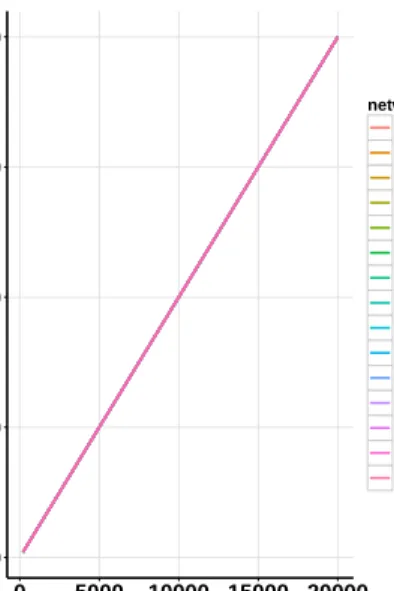
6.1 Two types ofsDNAsubscribed by 5 nodes (The lines do not represent edges in the graph andsDNAs are not nodes. The arrows define subscription or common preferences of different nodes assDNAs). . . 82 6.2 CPU vs GPU computation time with varying number of features. (CPU: Intel(R)
Xeon(R) W3680 @ 3.33GHz 6 cores and 12 threads, system memory: DIMM DDR3- 20 GB, GPU: NVIDIA GeForce GTX 1080Ti) . . . 87 6.3 Kernel density estimation of the underlying distribution for the properties of the
generated 4200 networks . . . 90 6.4 Real-world network properties (distribution). NDD: node degree distribution,
ASP: average shortest path, TD: local transitivity (clustering coefficient) distri-bution . . . 96 6.5 Snapshot-0 of the selected simulated networks. Network properties
(distribu-tion). NDD: node degree distribution, ASP: average shortest path, TD: local transitivity (clustering coefficient) distribution . . . 97 6.6 Snapshot-1 of the selected simulated networks. Network properties
(distribu-tion). NDD: node degree distribution, ASP: average shortest path, TD: local transitivity (clustering coefficient) distribution . . . 98
6.7 Snapshot-2 of the selected simulated networks. Network properties (distribu-tion). NDD: node degree distribution, ASP: average shortest path, TD: local
transitivity (clustering coefficient) distribution . . . 99
7.1 Global clustering coefficient for the simulated network datasets and real-world datasets (the real-world network’s global clustering coefficient measures are measured by Lee et al. (2014)) . . . 109
7.2 Snapshot-0 of the selected simulated networks. Network properties (distribu-tion). NDD: node degree distribution, ASP: average shortest path, TD: local transitivity (clustering coefficient) distribution . . . 111
7.3 Snapshot-1 of the selected simulated networks. Network properties (distribu-tion). NDD: node degree distribution, ASP: average shortest path, TD: local transitivity (clustering coefficient) distribution . . . 112
7.4 Snapshot-2 of the selected simulated networks. Network properties (distribu-tion). NDD: node degree distribution, ASP: average shortest path, TD: local transitivity (clustering coefficient) distribution . . . 113
7.5 Node label prediction accuracy (in fractions i.e. 0.7 implies 70% accuracy and the top horizontal bar show colour map for accuracy) from different Models (average from 10-fold cross-validation), networks are inX axis and models in Y axis. Models written as, F- feature only,T - topology only, F T - both the feature and topology,F T vanilla- the original GCN. Models withSin the right box (the blue outlined boxes) represents if an additional feature weight matrix in the first layer (Equation 7.16). The left box shows results for models that use graph representativeG =Lsym˜ , Equation 7.1 (i.e. adjacency matrix). The middle box usesGN S = ˜LsymN S, where N Sis a node-similarity (Katz,RP R, and GG) measure with different thresholds ( Equation 7.9, 7.11 and , 7.13). Similarity-basedGis preprocessed based on Section 7.2.2. The preprocessing threshold auto implies automatic selection of a threshold based on the mean value of the Aˆ (Section 7.2.2). All the networks are represented in terms of snapshots. For example, 0-0, is the first network’s first snapshot, 0-1 is the first network’s second snapshot. . . 118
A.1 S&N ei=2 . . . 131 A.2 S&N ei=4 . . . 132 A.3 S&N ei=8 . . . 133 A.4 S&N ei=16 . . . 134 A.5 S&N ei=2 . . . 135 A.6 S&N ei=4 . . . 136 A.7 S&N ei=8 . . . 137 A.8 S&N ei=16 . . . 138 A.9 S&N ei=2 . . . 139 A.10S&N ei=4 . . . 140 A.11S&N ei=8 . . . 141 A.12S&N ei=16 . . . 142 A.13S&N ei=2 . . . 143 A.14S&N ei=4 . . . 144 A.15S&N ei=8 . . . 145 A.16S&N ei=16 . . . 146
A.18 plotPredictions() auto-generating plots and statistics from experiment outputs
that had been auto-generated by calcPredictions() function . . . 149
A.19 PR AUC ofcollegeMsg dataset . . . 150
A.20 PR AUC ofcontactdataset . . . 151
A.21 PR AUC ofhep-thdataset. . . 152
A.22 PR AUC ofhep-phdataset . . . 153
A.23 PR AUC ofhypertextdataset . . . 154
A.24 PR AUC ofinfectiousContactdataset . . . 155
A.25 PR AUC ofMITContactdataset . . . 156
A.26 PR AUC heatmap of 7 datasets . . . 157
A.27 PR AUC barplot of 7 datasets. . . 158
A.28 PR AUC ofcollegeMsg dataset . . . 159
A.29 ROC AUC ofcontactdataset . . . 160
A.30 ROC AUC ofhep-thdataset . . . 161
A.31 ROC AUC ofhep-phdataset . . . 162
A.32 ROC AUC ofhypertextdataset . . . 163
A.33 ROC AUC ofinfectiousContactdataset . . . 164
A.34 ROC AUC ofMITContactdataset . . . 165
A.35 ROC AUC heatmap of 7 datasets . . . 166
A.36 ROC AUC barplot of 7 datasets. . . 167
A.37VirtualSoc, Simulation of a single network . . . 169
4.1 Average shortest path length of small-world networks with deleted and not deleted edges forp= 0.3andN ei= 16. Each of the networks are sampled 30 times. . 39 4.3 Number of simulated networks.. . . 40 4.2 Number of edges for different values ofSandN ei . . . 40 5.1 Prediction value for a simple graph in Figure 5.1. . . 52 5.2 Similarity measures with parameters, Common Neighbours (CN), AdamicAdar
(AA), Preferential Attachment (PA), Rooted PageRank (RPR), Average Com-mute Time (ACT), Average ComCom-mute Time Normalised (ACTN), Pseudoin-verse of the Laplacian matrix (PsInLap), Local Path Index (LPI), Leicht-Holme-Newman Global Index (LGI), and Matrix Forest Index (MFI) . . . 53 5.3 Basic statistics of the datasets selected for the experiment . . . 57 5.4 AUC for Katz with different centralities. Highlights in dark grey represent that
Inequality 5.6 holds (no such case exist in this table), and light grey represents AUC values lower than the AUC of a random predictor. . . 63 5.5 AUC for AdamicAdar (AA) with different centralities. Highlights in dark grey
represent that Inequality 5.6 holds (no such case exist in this table), and light grey represents AUC values lower than the AUC of a random predictor . . . 63 5.6 AUC for Common Neighbours (CN) with different centralities. Highlights in
dark grey represent that Inequality 5.6 holds, and light grey represents AUC values lower than the AUC of a random predictor . . . 64 5.7 AUC for Jaccard’s Coefficient (JC) with different centralities. Highlights in dark
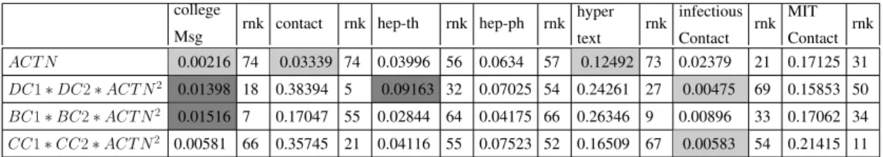
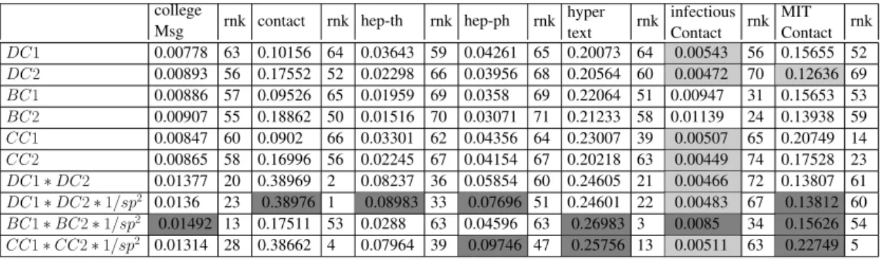
grey represent that Inequality 5.6 holds, and light grey represents AUC values lower than the AUC of a random predictor . . . 64 5.8 AUC for Average Commute Time (ACT) with different centralities. Highlights
in dark grey represent that Inequality 5.6 holds, and light grey represents AUC values lower than the AUC of a random predictor . . . 65 5.9 AUC for Average Commute Time Normalised (ACTN) with different
centrali-ties. Highlights in dark grey represent that Inequality 5.6 holds, and light grey represents AUC values lower than the AUC of a random predictor . . . 66 5.10 AUC for Rooted PageRank (RPR) with different centralities. Highlights in dark
grey represent that Inequality 5.6 holds, and light grey represents AUC values lower than the AUC of a random predictor . . . 66 5.11 AUC for Pseudoinverse of the Laplacian matrix (PsInLap) with different
cen-tralities. Highlights in dark grey represent that Inequality 5.6 holds, and light grey represents AUC values lower than the AUC of a random predictor . . . 67 5.12 AUC for Local Path Index (LPI) with different centralities. Highlights in dark
grey represent that Inequality 5.6 holds, and light grey represents AUC values lower than the AUC of a random predictor . . . 67
5.13 AUC for Leicht-Holme-Newman Global Index (LGI) with different centralities. Highlights in dark grey represent that Inequality 5.6 holds, and light grey repre-sents AUC values lower than the AUC of a random predictor . . . 68 5.14 AUC for Matrix Forest Index (MFI) with different centralities. Highlights in
dark grey represent that Inequality 5.6 holds, and light grey represents AUC values lower than the AUC of a random predictor . . . 68 5.15 AUC for Shortest path with different centralities. Highlights in dark grey
rep-resent that a combination method performs better than PA, and light grey repre-sents AUC values lower than the AUC of a random predictor . . . 69 5.16 Methods which satisfy Inequality 5.6. The dataset(s), in which a method
sat-isfied Inequality 5.6 is marked as Y, and the rank of that method mentioned in the parenthesis, i.e. Y(rank). First best score is marked with ***, second best with** and third best with *. For all the scores, higher is better. The ‘+’ operator entails a combination based on the Equation 5.2.. . . 71
6.1 Range of input parameters for the simulated networks. Generated from the sam-pling approach developed by Saltelli (2002) (Saltelli et al. 2010; Herman et al. 2014) for global sensitivity analysis. . . 89 6.2 Input parameters of the simulated networks. The parameters are: exploration
probabilityp, popularity preference intensityr, node-pair fraction connectiont, path 2 preference intensityc1, path 3 preference Intensityc2, path 4 preference
intensityc3 . . . 93
6.3 Properties of simulated and real-world networks. Simulated networks are
repre-sented as numbers (https://www.kaggle.com/akandaashraf/virtualsoc1
to download the datasets). GCC - Global Clustering Coefficent , CCS - Clustering Coefficent Standard Deviation, CDM Centrality Degree Mean, CCM -Centrality Closeness Mean, CDS - -Centrality Degree Standard Deviation, CCS - Centrality Closeness Standard Deviation, AGPL - Avg Geodesic Path Length. The real-world networks Facebook and Google Plus are friendship based ego networks (Leskovec and Mcauley 2012;Facebook (nips) network dataset KONECT
2017; Google+ network dataset – KONECT 2017). Twitter (De Choudhury et al. 2010;Twitter lists network dataset KONECT,2017) containing informa-tion on who follows whom on Twitter. The Hamster network is a full network containing friendships and family links between users of the website hamster-ster.com (Hamsterster full network dataset KONECT2017) . . . 95 7.1 Models used along with the original GCN. All of the models with features are
trained twice, once with the weighted feature matrix in Equation 7.16 and once without . . . 114 7.2 Two citation networks’ statistics (Kipf and Welling 2017) . . . 115
7.3 Accuracy of correctly predicting node labels (ACC) and standard deviation (SD) of the best vs original GCN model. Models written as: F- features only, T -topology only,F T- both features and topology,F T vanilla- the original GCN. S in the right column denotes usage of an additional feature weight matrix in the first layer (Equation 7.16). The models that useGN S = ˜LsymN S, whereN S
is a node-similarity (Katz,RP R, andGG) measure with different thresholds (Equation 7.9, 7.11 and, 7.13) are represented in the last column with the corre-sponding node-similarity matrix (e.g. katz for the model FTkatz0.0-0.5). All the similarity-based G are preprocessed and reconfigured based on Section 7.2.2. The preprocessing threshold auto implies automatic selection of a threshold based on the mean value of the normalised node-similarity matrix (as per Sec-tion 7.2.2). Networks are represented in terms of snapshots, e.g. 0-0: first network’s first snapshot, 0-1: first network’s second snapshot etc. . . 120 7.4 Accuracy (ACC) and standard deviation (SD) of the models with 46 random
weight initialisation on two citation networks,CoraandCiteseer. Models writ-ten as: F- features only, T- topology only, F T- both features and topology, F T vanilla- the original GCN.Sin the right column denotes usage of an addi-tional feature weight matrix in the first layer (Equation 7.16). The models that useGN S = ˜LsymN S , whereN Sis a node-similarity (Katz,RP R, andGG)
mea-sure with different thresholds (Equation 7.9, 7.11 and, 7.13) are represented in the last column with the corresponding node-similarity matrix (e.g. atz for the model FTkatz0.0-0.5). All the similarity-basedGare preprocessed and recon-figured based on Section 7.2.2. Models withSrepresents if an additional feature weight matrix in the first layer (Equation 7.16). First best accuracy is marked with ***, second best with** and third best with *. . . 121 7.5 Accuracy (ACC) and standard deviation (SD) of the models with 100 random
splits on two citation networks,CoraandCiteseer. Models written as: F- fea-tures only, T- topology only, F T- both features and topology, F T vanilla -the original GCN.S in the right column denotes usage of an additional feature weight matrix in the first layer (Equation 7.16). The models that useGN S =
˜
LsymN S , where N S is a node-similarity (Katz, RP R, and GG) measure with different thresholds (Equation 7.9, 7.11 and, 7.13) are represented in the last column with the corresponding node-similarity matrix (e.g. katz for the model FTkatz0.0-0.5). All the similarity-based Gare preprocessed and reconfigured based on Section 7.2.2. Models withSrepresents if an additional feature weight matrix in the first layer (Equation 7.16). First best accuracy is marked with ***, second best with** and third best with *.. . . 122
A.1 ROC AUC Ranked . . . 168 A.2 Properties of the 7 datasets . . . 169 A.3 Input parameters for the simulated networks in Chapter 7, Figure 7.5 and
Ta-ble 7.3. 1400 networks are simulated using this sampling method and the first ten networks with the above first ten parameters are used in 7. Each of the networks is consists of three snapshots, thus 30 networks in total . . . 171 A.4 Properties for the simulated networks used in Figure 7.5 and Table 7.3. Each of
Introduction
“Networks are everywhere”, among all the different types of networks (e.g. social, biologi-cal, internet, road networks, etc.) interest in social networks has experienced particularly rapid growth, mainly due to the availability of large real-world network datasets (Liben-Nowell and Kleinberg 2007;Brandes et al. 2013;Barab´asi and Bonabeau 2003). Research in social net-works, leveraging these large-scale data, is mainly focused on patterns and evolution of the social structure. According to Freeman et al. (1987), “social structure refers to a relatively prolonged and stable pattern of interpersonal relations”. Although large-scale social networks analysis is ubiquitous nowadays, the groundwork in the shape of small-scale social network analysis began long before the era of MySpace or Facebook. The origin of network science can be traced back to the 18th-century scholar Euler, who introduced graph theory (Euler 1999). However, for social networks, the field which had been previously known associometryis now transformed into social network analysis and has become a part of much broader research area called network science. The study of social network dynamics could be found as early as 1934 whenMoreno(1934) designed a hand-drawn friendship diagram. However, this social network is minimal when compared with today’s hundreds of millions or even billions of nodes in online social networks like Facebook and Twitter. From that friendship diagram, Moreno(1934) in-ferred simple conclusions that there were more friendships or connections between the same gender than opposite genders. Although these findings are relatively straightforward and intu-itive, the study had pioneered today’s social network analysis. The friendship diagram analysis byMoreno(1934) demonstrated that social behaviour can be understood more easily when the interactions are represented in the form of a diagram, i.e. a network.
A network is typically represented as a graph and consists of a set of connected entities. In the field of network science, following from the graph theory, these entities are referred to as nodes or vertices while the connections between them are known as edges or links (Newman 2010a). A network could be defined by itsEedges andV vertices. The evolution of societies is
captured, mainly, through the emergence and disappearance of nodes and edges in the network that is a representation of complex system – in here a society. However, changes in the node and edge attributes also reflect the evolution of societies. Thus, analysis of such network could give a broader understanding of the evolution of societies. The field of network science could also be thought of as the study of the collection, management, analysis, interpretation, and presentation of relational data (Brandes et al. 2013). Another large quantity of network science work is also dedicated towards mathematical modelling of the networks (Barab´asi and Bonabeau 2003; Erd¨os and R´enyi 1959;Watts and Strogatz 1998). Network science is still an emerging field as more and more complex and large-scale network data becomes available. Network science does not belong to a single discipline but is a combination of multiple disciplines, including graph theory, physics (statistical mechanics), data mining and sociology (Brandes et al. 2013; Tiropanis et al. 2015).
Due to the availability of large-scale network data, for the first time in history, we have the pos-sibility to process ‘big data’ (gathered by computer systems) about the interactions and activities of millions of individuals. It represents an increasingly essential yet under-utilised resource be-cause due to the scale, complexity and dynamics, Complex Social Networks (CSN) extracted from this data are extremely difficult to analyse. A coherent and comprehensive approach to analyse such networks and their dynamics is crucial to advance our understanding of people’s continuously changing behaviour. Networked systems and their evolution are usually analysed by building models of interactions using the classic random, scale-free, and small-world models. However, these do not precisely reflect the complex nature of real-world networked systems and their dynamics.
To develop predictive models for a social network, it is essential to recognise its complex topo-logical patterns and changes in those patterns with respect to time. In the majority of complex networks, three aspects affecting the whole network, can typically change. These are (1) changes in links (e.g. emergence and disappearance), (2) changes in nodes (e.g. emergence and dis-appearance of nodes), and (3) changes of properties/features (of both nodes and links). This project, firstly, focuses on the first type of changes listed above, i.e. changing the number of relationships (emergence of links).
A social network dataset with topological information only, can contain enough information for predicting future relationships with better than random accuracy (Liben-Nowell and Kleinberg 2007). The complex structure or topology of a social network includes information which is not visible to the naked eye but can be used to make predictions for future interactions (e.g. link prediction based on the intrinsic topological patterns). This predictability from topology of the network only, is a very intriguing aspect of the data with relational components. We discuss our approach to the link prediction problem in Section 1.1. Secondly, going further than predict-ing relationships based on topology only, in this research, the topology of a network is fused
with the node features for the prediction of node labels (e.g. a person’s political views in so-cial networks). This type of classification problem is formally known as the node classification problem for networks. Attributes like gender, political preferences or age are a few examples of the standard node features in social networks. In this thesis we also work on the area of node classification in social networks. Elaborated in Section1.2, our work on the node classification domain also indirectly leverages the link prediction problem for social networks. In the famous study byLiben-Nowell and Kleinberg(2007), it has been discussed that the link prediction prob-lem in social networks is related to the probprob-lem of predicting missing links. Although missing link prediction and link prediction may sound similar, there are subtle differences between these two concepts (based on the upper bound of the kind of problems they deal with). In a missing link prediction task, it is assumed that there are hidden interactions between nodes that need to be inferred. Whereas in a link prediction task, the goal could also be predicting missing links but in combination with the main goal of predicting links which are likely to be formed in future. In other words, a link prediction can be thought of as forecasting links, whereas a missing link prediction does not deal with the time dimension. Perhaps, it can also be argued that the missing link prediction problem is a subset of the link prediction problem. An example of link predic-tion could be future friend predicpredic-tion in social networks, whereas, an example of the missing link prediction is, predicting suspicious interactions in a mobile network which the users are trying to hide. Hence, although, most of the existing link prediction and missing link prediction techniques can be used interchangeablyLiben-Nowell and Kleinberg(2007), the difference in their underlying problem-specific concepts, their precise theoretical benefits become more ap-parent for a particular application. For the node classification problem, use of the concept of missing link prediction makes more sense (as opposed to the link prediction problem), based on the argument that we are inferring already existing hidden interactions of the network. These hidden interactions can be predicted for a richer representation of the network, which interns, increases the performance of the node classification task (a more detail explanation is given in Section1.2). In our node classification related contributions, we make use of this very notion of mission link prediction (see Section 1.2). This concept of missing link prediction can be useful for the task of recognising node patterns in networks which is termed as the classifica-tion problem. The difference between the classificaclassifica-tion problem for datasets with the relaclassifica-tional components (i.e. networks) and without the relational components is that the relational elements contain intricate and potentially useful topological information. These topological patterns are crucial elements of the datasets for any predictive modelling applied to networked data. If a pre-dictive model for networks does not consider these topological patterns, it can under-utilise the available information within the datasets, leading to suboptimal performance. In this work we show that these relational components can be further enhanced using our proposed approaches in Chapter7which are based on the concept of missing link prediction.
1.1
Link Prediction
As discussed earlier, the prediction of social relations, i.e. the link prediction is one of the most essential parts of the evolution of a social network, alongside new node appearance. This link prediction is the first goal of this project. The existing techniques for link prediction are discussed in Chapter2. Developing new link prediction techniques or improving the existing approaches firstly requires identifying the main contributing factors to the formation of new links. The second step is to determine how to combine or utilise these contributing information for a better link prediction method. In this thesis two main contributing factors to link prediction are identified from the literature, namely popularity and similarity (Papadopoulos et al. 2012; Thwe 2013). The popularity of a node implies how popular or influential a node is in a social network, whereas similarity implies how similar two nodes are. Popularity can be measured using Centralities, such as the Degree Centrality and similarities can be measured using shortest path length between two nodes and other widely used similarity measures such as Katz, Rooted PageRank etc. This work proposes to combine these two contributing factors using a law found not necessarily in the social science but in the natural world, namely Newton’s law of universal gravitation.
If we consider a social network, at its local level, how two people make a connection or inter-act could rely on two finter-actors, (1) how popular, and (2) how similar these people are. These two concepts are well established in the link prediction paradigm (Papadopoulos et al. 2012; Thwe 2013). Intuitively, for social networks, predicting the appearance of links between two people, having both the popularity and similarity factors should entail better prediction accuracy than considering only one of these factors. In social networks, we already have a wide range of measures for calculating the popularity of nodes and similarities between them. Different centrality measures (e.g. degree centrality, closeness centrality or betweenness centrality) could be thought of as notions of popularity. On the other hand, scores from link prediction methods like Katz or AdamicAdar could be thought of as measurements of nodes’ similarity (Freeman 1977;Katz 1953;Adamic and Adar 2003). However, the challenge is how to combine these two types of metrics in order to predict links between two particular nodes in the future. This is where we make use of Newton’s law of gravity. In Newton’s explanation of gravity, the force between two particles is proportional to the product of their masses and inversely proportional to the squared distance between them. We argue that this law of attraction between two point masses could also be applicable in social networks. We measure the popularity or importance of a node using centrality and consider it as mass. We measure dissimilarity by the inverse of similarity (i.e. scores from link prediction methods like Katz, AdamicAdar etc.) or by the path length, and consider them as distance. The detailed theoretical and empirical analysis of this novel Newtonian gravity inspired method is described in Chapter5.
1.2
Missing Links and Node Classification
A link prediction algorithm typically predicts future links based on the current information avail-able within the network. However, link prediction methods (many of them measure node similar-ity) can also be categorised as predicting missing links for a network at the current time (i.e. not for a future snapshot) (Liben-Nowell and Kleinberg 2007;Goldberg and Roth 2003;Popescul and Ungar 2003;Taskar et al. 2004). A link prediction method infers links which are not directly visible within the network but have a high likelihood of forming in the future (Liben-Nowell and Kleinberg 2007). This consideration of node similarities as missing links can address some of the limitations of the Graph Convolutional Network (GCN) (Kipf and Welling 2017), a state-of-the-art method for node classification, which we discuss in Chapter7. GCN has been shown to outperform other state-of-the-art models on citation networks and a knowledge graph for the task of node classification. The GCN can efficiently combine the graph topology with the node features for the task of node classification. However, the mentioned limitation for the GCN is that at a particularlthlayer of the neural network model, it can only consider up to thelthorder of neighbourhood of nodes as influential, which may not always hold. This strong dependency between the highest layer and the size of node-neighbourhood can limit the node classification accuracy, especially for friendship-based networks. This is because, for a given node, a distant node (i.e. not directly connected) may have higher similarity than the directly connected nodes. These similarities between two distant nodes indicate that they will likely connect in the future, which in turn implies a missing link between them. In the work where GCN has been introduced byKipf and Welling(2017), it has been applied and benchmarked for citations and knowledge networks. Thus, the evaluation of the full potential of the GCN on a friendship-based social network also requires openly available datasets in larger quantities. However, most available social network datasets are not complete (i.e. they represent a subset of the original networks e.g. ego-networks, not the entire graph or do not include the entire set of node features1). On top of that, the majority of the available social network datasets not only do not contain any features but also ground truth labels. Although there are mathematical models available for gen-erating graphs, these do not generate features and labels, thus only the topology of the graph is obtainable. To address the need for good quality synthetic social network data with ground truth labels and features we provide a guideline on how to simulate dynamic social networks, with ground truth labels and features, both coupled with the topology of the network (Section1.3). We then use three node-similarity measures, our Newtonian gravity inspired method coined as the Graph Gravity (GG), Katz and, rooted PageRank to increase node classification accuracy of the GCN. The models based on the combination of these similarity measures with a unique data reconfiguration technique outperform the original GCN model in 27 out of 30 simulated datasets that we have used. They also outperform or match the original GCN on two real-world
1
citation network datasets. Additionally, we have proposed another variation of the GCN, which includes a weight matrix to learn the strength of each feature for defining the node labels for all the nodes. Chapter7includes the detailed discussion about these four new deep learning models based on the GCN concept.
1.3
Social Network Simulation
As mentioned in Section1there is now an unprecedented availability of social network datasets, however, most of the openly available datasets are not complete, i.e. they only represent subsets of bigger networks and/or do not contain node attributes. One major limitation of the neural network-based learning systems is that they require a large amount of data for training. This is one of the most significant differences between human intelligence and artificial non-general intelligence like an artificial neural network. Unlike a deep learning (i.e. deep neural network) model, a human can learn from a minimal number of examples, whereas a deep learning model requires to see a substantially larger number of samples to learn. Thus, it is essential to have access to a large number of training data instances to unlock and evaluate the full potential of the neural network-based model. A straightforward technique to solve this problem of insufficiency of the high quality real-world datasets for neural network-based learning systems is to simulate high quality real-world alike synthetic data and use it to train the model. Additionally, if not for training, simulated datasets are particularly useful to evaluate the models’ performance, i.e. dur-ing the testdur-ing phase. In many cases, it is far more convenient to simulate test cases representdur-ing exceptional situations than collecting data for those situations in the real world. In fact, for some real-world scenarios, it might not even be possible to get a dataset describing some exceptional scenarios due to the rarity of the event or ethical constraints.
It is, however, crucial to test the trained model in those exceptional scenarios because the cost of failure for those unlikely situations can be significantly higher than a regular situation. One such area where high quality simulated and augmented data is extensively being used is in the neural network-based learning systems for self-driving cars. Almost all advanced autonomous vehicle technologies use simulated datasets. For example, Nvidia has developed the Nvidia Drive Constellation, a Virtual Reality Autonomous Vehicle Simulator (NVIDIA n.d.). Billions of miles have been driven in the simulated environment by Google’s Waymo (Waymo n.d.) etc. Similar to the self-driving cars, in many other applications of deep learning, high quality simulated datasets are now in high demand.
With the advancement of graph specific neural network-based models, the demand for such datasets is growing rapidly. Furthermore, it is becoming more and more difficult to have access to complete (i.e. inclusive of node attributes) datasets representing social networks mainly due to user privacy concerns that we discuss later in this section.
Social network datasets are very complex in nature, thus, they can be difficult to simulate and there is a lack of comprehensive guidelines on how to simulate social network datasets with both the features and ground truth labels.
As mentioned earlier, graph data mining has become an active research area due to the recent advancement and popularity of social networks (Wasserman and Faust 1994;Newman 2018), especially the online ones. Advancements in graph-based predictive modelling or graph commu-nity detection algorithms require datasets with ground truth labels for evaluation purposes ( Sa-pountzi and Psannis 2018). However, the majority of the available social network datasets do not contain labels. Moreover, real-world social network datasets contain high dimensional fea-tures (Pecli et al. 2018) that represent information about both nodes and relationships. For example, a Facebook user generates a variety of information such as posts he/she likes, photos, status updates, etc. Even in citation networks, there are features such as the domain, authors’ affiliations, documents with thousands of words, etc (Popescul and Ungar 2003). In publicly available datasets, such features are rarely included.
This is due to the fact that during the anonymisation process of networked data, in most cases we need to get rid of the majority of features as these could be used to identify individu-als (Townsend and Wallace 2016), potentially raising ethical concerns. De-identification of network datasets is particularly tricky because of the unique topological structure a network may have. In a 2011 Kaggle link prediction competition, the winning team successfully de-identified most of the network data by matching the anonymised network topology with the real network, instead of using the actual link prediction algorithm (Narayanan et al. 2011). On top of that, nowadays, even such graph datasets are becoming very difficult to obtain due to the aftermath of the notorious usage of the real-world dataset from social networks for the purpose of political influence (Hand 2018;Cadwalladr and Graham-Harrison 2018).
One of the infamous recent developments in data misuse is that around 50 million Facebook users’ profiles have been analysed without their consent by Cambridge Analytica, a British political consulting firm. Moreover, it has been claimed that the data analysis was performed in order to influence the outcome of 2016’s US election (Cadwalladr and Graham-Harrison 2018). This incident of the data breach along with many others, has ignited a backlash from social network users and politicians.
To ensure user’s data is only used with explicit consent, governments and political unions are increasingly putting pressure on the technology companies on protecting user’s data (Quinn 2018). Additionally, new regulations, such as the European General Data Protection Regulation (GDPR) on the usage of personal data, have already come into force in many countries, such as the UK (Bennett 2018). Unquestionably, such regulations are essential to guarantee user privacy. However, as a result, availability of datasets from social media in the public domain is sharply declining. Maintaining the advancement of the research in social networks requires good quality
real-world datasets. One solution is to supplement the real-world social network datasets with synthetic, good quality, real-world alike data.
Typically, a link prediction algorithm is tested based on its predictive power on a future snapshot of the network. A supervised link prediction algorithm should ideally utilise both the topology and available node attributes (Lichtenwalter et al. 2010;Pecli et al. 2018). For example, Scel-lato et al. (2011) found that including features such as places and other related user activity improves the accuracy of link prediction considerably. Most of the developments in link predic-tion have been based on a single snapshot of the network, although, incorporating the evolupredic-tion of the graph may result in better performance in link prediction as shown by Tylenda et al. (2009) andXu et al.(2018).
To address the need for openly available high-quality social network datasets, we have intro-duced an open-source Python-based social network simulation library with GPU computation and multiprocessing. In our social network simulation, we argue that the topology of the net-work is driven by a set of latent variables, termed as the ‘social DNA’ (sDNA), which define the preference of nodes towards the features of other nodes, and which are not necessarily ex-clusive to a single node, whereas the single node’s entire set of features is. We consider the
sDNAas labels for the nodes, mimicking the real-world social network scenario. We describe our simulation process along with the validation of the simulated datasets in Chapters6and7.
1.4
Original Contributions and Outputs
1.4.1 Research Contribution
The four main research contributions of this thesis are:
1. In depth comparison and analysis of the three classical network models (random, small-world and scale-free networks models), leading to new insights on how different these three network models’ properties (many of these properties do not have analytical so-lutions) are, for a fixed-size network. This has also laid the foundation of our network simulation framework in Chapter8.
2. Development of a class of new nature inspired and robust link prediction approaches called Graph Gravity (GG). The proposed link prediction algorithms have better predictive power when compared with many of the existing link prediction methods.
3. Combining graph theory based link prediction with modern deep learning models in a coherent approach, resulting in development of four new node classification algorithms, outperforming the existing methods.
4. Comprehensive social network simulation framework, able to jointly model network topol-ogy and node features.
This thesis has several research outputs including, high-quality publications and open-source software developed in order to disseminate the research findings. Following are the publications resulting from the research presented in this thesis:
1. Wahid-Ul-Ashraf, A., Budka, M. and Musial-Gabrys, K., 2017, November. Newton’s gravitational law for link prediction in social networks. In International Conference on
Complex Networks and their Applications(pp. 93-104). Springer, Cham.
DOI:https://doi.org/10.1007/978-3-319-72150-7_8
Chapter:5
2. Wahid-Ul-Ashraf, A., Budka, M. and Musial, K., 2018. NetSim – The framework for complex network generator.Procedia Computer Science, 126, pp.547-556. DOI:https: //doi.org/10.1016/j.procs.2018.07.289
Chapter:4
3. Wahid-Ul-Ashraf, A., Budka, M. and Musial, K., 2019. How to predict social relation-ships – Physics-inspired approach to link prediction. Physica A: Statistical Mechanics
and its Applications, 523, pp.1110-1129.
DOI:https://doi.org/10.1016/j.physa.2019.04.246
Chapter:5
4. Ashraf, A.W.U., Budka, M. and Musial, K., 2019. Simulation and Augmentation of Social Networks for Building Deep Learning Models.Preprint.
arXiv Preprint:https://arxiv.org/abs/1905.09087
Chapter:6,7
5. Ashraf, A.W.U., Budka, M. and Musial, K., 2020. SocialDNA - Capturing Complex Nature of Human Behaviour in Social Networks.Submitted, Scientific Reports.
Chapter:6
There are three software libraries that have been developed during this project, two of which have been made open-source:
1. NetSimis developed in R to robustly (i.e. comparing many different parameter settings for
each of the models) compare properties of three network models with different sizes and density. The library can generate networks with any given set of parameters and relevant reports for analysis. The code has been made open-source. The GitHub repository for the
code:
https://github.com/AkandaAshraf/netsim
2. LinkPrediction, an R library to benchmark and evaluate the new link prediction technique
along with 12 other widely used link prediction methods. The software library uses multi-threading to optimise the performance. This library is now also being used by the under-graduate students in the University of Technology Sydney as a part of their coursework in Computing Science Studio and Research Projects.
3. VirtualSocis a software developed in Python 3 to generate dynamic synthetic social
net-work datasets with ground truth labels and features. There are two versions of this soft-ware, one for the CPU and another one for the GPU. No other network analysis library has been used to develop this software. The source code is available under the MIT license. The GitHub repository for the package can be accessed using the following link:
https://github.com/AkandaAshraf/VirtualSoc
1.5
Thesis Structure
FIGURE1.1: The relation between research domains, concepts, and Chapters4-7
This thesis is organised as follows. In Chapter2we discuss related work and also propose a new categorisation of the link prediction methods. Chapter3is where we describe the methodology of the study, including the research questions, objectives, and tasks that have been undertaken to fulfil those objectives. Chapter 4 includes the analysis of different network models, sizes, densities and properties. We then describe the new link prediction methods with empirical
analysis in Chapter5. Afterwards, a comprehensive network simulation framework is presented in Chapter 6 which is developed primarily based on our understanding of the three network models from Chapter4. In Chapter7, we validate the simulated networks and propose four new variants of the GCN. Finally, in Chapter 8 we conclude this thesis, also outlining future research directions. This thesis also includes an AppendixAwith additional figures, statistics and information on the developed software libraries.
Literature Review
In this chapter, different properties of a network are introduced from literature which is related to Chapter 4 where the behaviour of these properties with respect to different size and types of networks are analysed. Understanding these network properties are essential to any network analysis or modelling. After introducing the network properties, the focus is then shifted to network evolution in the form of link prediction. Also, the importance of link prediction from literature is brought forward in this chapter. In Chapter5, a new physics inspired link prediction method is proposed. Literature related to this physics inspired link prediction are then pointed out. Additionally, the classification of the link prediction method is proposed in this chapter. A number of link prediction methods are then discussed in this chapter. Afterwards, different network models are presented which is relevant to the network simulation process in Chapter6.3 and7. These three network models are essential for the development of our network simulation library in Chapter4and6.3. Finally, the Graph Convolutional Networks (GCNs) are discussed related to the four proposed new variants of the GCNs models that are developed and designed in Chapter7.
2.1
Properties of Networks
There are different properties and measures of network characteristics, some of them are very easy to calculate precisely while others are must be estimated. They give insights and help infer essential properties of a network (Newman 2010a;Costa et al. 2007).
The two most important and straightforward measurements of networks are Degree and Shortest path.
Degree and degree Distribution: One of the most essential and fundamental properties of a network is its degree distribution. The degree of a node is the number of edges connected to it
and histogram of the degree of each node is the degree distribution of that network (Costa et al. 2007).
Shortest Path: The shortest path between a pair of vertices are called shortest path for that pair of vertices. In a whole network, the average shortest path could be calculated by taking the average of all shortest paths between all pairs of vertices. It could be calculated through breadth-first search (Dreyfus 1969). The shortest path is also known as the geodesic path (Newman 2010a).
Diameter:The longest shortest path in a network is known as the diameter of a network ( New-man 2010a).
Transitivity:Transitivity is a critical concept, mainly for social networks. This is because high-level transitivity seems to be a very apparent feature of a social network (Newman and Park 2003). Transitivity was first introduced by (Newman 2001b). A straightforward explanation of transitivity could be that friend of my friend is also my friend. Perfect transitivity only occurs in a clique where three vertices form a fully connected subgraph. If A is connected to B, B is connected to C, and C is also connected to A then it could be said that this subgraph of A, B, and C forms a clique which is a perfect transitivity. If vertex C and A are not connected then A, B, and C are partially transitive. If A knows B, B knows C then we have a path of ABC of two edges in the network. If now A knows C then we have the triad. Clustering coefficient1 in a
network is the measurement of triads.
The Clustering Coefficient, C is measured using the following formula:
C = number of closed path of length two
number of paths of length two (2.1)
In Equation2.1, if C= 1, it implies perfect transitivity and all the components are cliques, c=0 implies no closed triads which indicates the network is a tree (Newman 2010a). In social net-work terms, it could be explained as the fraction of pairs with a common friend which are also friends with themselves.
C = number of triangles *3
number of connected triples (2.2)
Here in Equation2.2, three is multiplied because the connected triples are counted three times ( New-man 2001b). Equation2.2is also known as the fraction of connected triples. Socials networks usually have higher clustering coefficient when compared with other technological and biologi-cal networks (Mislove et al. 2007). The high value of clustering coefficient is thought to be due
to the fact that we do not pick our friends randomly, rather two people have higher chances of being friends if they have a common friend.
Clustering Coefficient for a single vertex:It is a measurement of how strongly the neighbours of a vertex A is connected between pairs (Watts and Strogatz 1998). It is measured via:
C= The number of pairs that are connected
number of pairs of the neighbours of A (2.3)
Equation2.3is called local clustering coefficient, and it has a rough dependence on the degree. Vertices with a higher degree have lower local clustering coefficient. This high local clustering coefficient is also an indicator of the structural hole (Butt 1992). The missing links between pairs of vertices are defined as structural holes. Structural holes are especially important in social networks. If we are interested in efficient information flow in a network, then this high clustering coefficient is undesirable. These structural holes reduce the number of alternative routes information can take through the network (Butt 1992). However, structural holes could also be a good thing, as having no connection between the adjacent pair of a vertex A means the adjacent pair have to connect via A which gives A the power to control information flow. In that sense, Structural holes could be a type of centrality measure as it defines the importance of a node in a network regarding controlling information flow. Centrality measures are discussed in later sections.
Mean Local Clustering Coefficient: Watts and Strogatz(1998) proposed a clustering coeffi-cient for the entire network as a mean of local clustering coefficoeffi-cients for each vertex.
2.1.1 Centrality
Vertex centrality measures are fundamental in network analysis. Centrality quantifies how im-portant or central vertices are in a networked system.
Degree Centrality: A simple, but perhaps the most crucial measure of centrality is the degree of vertices in a network. The degree of a vertex in a network is referred to the number of edges attached to it. Degree centrality is a handy measure of centrality in social networks.
Closeness Centrality:which is calculated based on the mean geodesic path from a given vertex to all other vertices in the network (Newman 2010b). High closeness centrality of a vertex means the vertex has better access to information or more direct influence on other vertices. Closeness centrality is defined as:
CC(vi) =
1 P
n6=id(vi, vn)
Here, dis the geodesic distance between two vertices. As it can be seen in Equation 2.4, if there are a totaln+ 1vertices in a graph, closeness centrality for vertexvi is calculated using
the inverse of the average length of the shortest path from/to all other vertices except itself vi 6∈ {v1, v2, ..., vn}. If the path does not exist between two vertices, then the total number of
vertices is used instead of path length (Csardi and Nepusz 2006).
Betweenness Centrality: this centrality gives a score to a vertexvi based on how many paths
connecting any two vertices in the network go through that vertexvi. If the number of those
paths is high, then vertexviwill have high betweenness centrality.
Vertices that are frequently on the shortest paths between any two vertices of the graph have more control over information flow (Freeman 1977;Anthonisse 1971). Removing a vertex with high betweenness centrality has a negative influence on the overall information flow in a network. The betweenness centrality is different from other centrality measures as it does not consider how well-connected a vertex is but it measures how much a vertex falls in between others. This way it is possible to have a vertex with a low degree but high betweenness centrality. For example, two groups of vertices can be connected via a single path and then a vertex that connects those groups (a.k.a. bridge node or broker) can have a high betweenness centrality. If a network has set of verticesV, source vertexs∈V and target vertext∈V, the betweenness centrality of vertexvican be defined as (Freeman 1977;Anthonisse 1971;Brandes 2001):
BC(vi) = X s6=vi6=t σst(vi) σst (2.5)
whereσst is number of shortest paths between two verticessandtandσst(vi)is the number of
shortest paths between two verticessandtthat passes through nodevi.
Eigenvector Centrality:This centrality measure could be thought of as a bit more complicated measure of degree centrality. In degree centrality, a vertex gets one point if it has one neighbour, but in eigenvector centrality, the neighbours also get a rating. This centrality measure was first proposed by (Bonacich 1987). Eigenvector centrality for a vertexviis,
vi =K1−1
X
j
AijXj0 (2.6)
Here,Mij is the an element of adjacency matrixM,K1 is the largest value from eigenvalues
Ki. To understand eigenvector centrality from a social network point of view, a person might
have few friends or connection but still, have high eigenvector centrality measure because most of his/her connections are very important or central (have higher centrality measure). Usually, the value of eigenvector centrality is not normalised. This centrality works best for undirected
networks for directed networks it arises complicacy. In directed networks, the outward con-nection from a node does not necessarily give importance to the node from which it is pointed outwards. For example, a web page has an outward connection to thousands of other pages, and some of them could be very important). To get around this problem the eigenvector centrality of an undirected network is measured by the number of inward connections. One big problem with this centrality measure in the directed network is if a vertex has many inward connections and those vertices also have connections pointed towards other vertices. If we encounter one or many vertex or vertices have no inward connection, in this case, we will get zero measure by using eigenvector centrality.
Katz Centrality (Katz 1953): This centrality measure solves the major problem that we face with eigenvalue centrality, the problem of zero centrality discussed earlier. This problem is solved via adding a free weight to every node. Although the Katz Centrality is proposed to deal with the problem with directed network but it can still be applied, and sometimes very useful in undirected networks. It allows a vertex to have high centrality regardless of their neighbour’s centrality measure if it has many connections.
vi =α
X
j
MijXj+βi (2.7)
In Equation 2.7, α andβ are positive constants. α is the eigenvector centrality, and it is the sum of centralities connecting to vertexi, andβ is the extra constant value that all the vertices receive by default.
PageRank: One drawback of Katz centrality is if a vertex has high centrality value and if it points to another vertex, then the pointed vertex gains more centrality. Let’s assume the case that, Facebook is pointed to millions of websites, so it has high centrality. However, if it points to a particular website, that website will gain centrality just because of Facebook has high centrality. Facebook is probably pointed to millions of other websites which are not particularly important. The idea behind solving this problem is by changing the centrality gain by dividing the gain by the vertices’ out-degree. This centrality is the core of web ranking technology, and Google gave its trade name PageRank (Brin and Page 2012).
vi =α X j Aij Xj Kout j +β (2.8)
In both Equations2.7 and2.8, the Katz and PageRank centrality there is a parameterα. This αparameter needs to be tuned. For undirected networks,αis less than one, and in the directed networks it is different, and in practical use usually, it is in the order of one. In PageRank, it is also possible to define different additive constant for different vertices.
2.2
Mesoscale Structures
One important aspect for the topology of social networks are their mesoscale structures, such as communities and core-periphery.
2.2.1 Communities
Community structures represent groups of nodes which have stronger interactions within them-selves, i.e. intra-interactions, but weaker interactions with nodes outside that community, i.e. weaker inter node interactions. In social networks, these interactions are formed via links or edges (Fortunato 2010;Lancichinetti et al. 2010). There are several ways to identify commu-nities in a graph. Identifying commucommu-nities requires algorithms which can infer the best parti-tions between different subgraphs, representing different communities. Modularity optimisation or more specifically maximisation is one such algorithm which can quantify communities in graphs. A modularity maximisation algorithm typically measures the quality of the communi-ties by finding a division of the network which gives the highest modularity. However, because the number of division of the network can be exponentially high, an exact solution is not practi-cal, thus an approximation of best modularities are inferred for detecting communities in a large graph (Newman 2016). Another pathway to detect or infer communities in a network is by using statistical inference. In statistical inference, one fits a generative network model to the observed network. Initially, a total ofnnumber of nodes is taken without any edges to attach to them, and then they are divided (using some stratigies (Newman 2016)) intoq groups. Then edges are independently attached between all the nodes at random. The difference of probability of edges being attached within the nodes in a group and between the groups gives fitness of score of the community structure (Newman 2016). For nodes in a community, the probability of edges being attached within themselves is expected to be higher than nodes which are in a different community.
2.2.2 Core-periphery
A core-periphery structure of network implies that the network consists of two different struc-tures, core and periphery. The core nodes are connected densely and the periphery nodes are sparsely connected (Da Silva et al. 2008;Borgatti and Everett 2000;Rombach et al. 2014;Zhang et al. 2015). A simple way to determine the core-periphery structure in networks is to divide the nodes based on their degrees. However, for more precise detection of the structure other algorithms such as fitting a stochastic block model (which fits the observations using expecta-tion–maximisation algorithms) can be used (Zhang et al. 2015).
In this work, we do not explicitly measure the above mentioned mesoscale structures. However, there is implicit consideration of these structures within this work. For example, the community detection techniques mentioned in Section2.2.1are unsupervised, however, there are modern deep learning approaches which can identify communities in a supervised or semi-supervised context, which we talk about later in Section 2.4 and in Chapter7 (Kipf and Welling 2017). For our link prediction algorithms developed in Chapter5, we consider methods such ask Katz, rootedPageRank, Average Commute Time (ACT), and they implicitly consider the surrounding of a pair of nodes to predict link formation (Katz 1953;Brin and Page 2012;L¨u and Zhou 2011). These surroundings generally contain information of the connectedness of nodes, thus consid-ering the mesoscale structure. For example, if a pair of nodes’ surrounding neighbourhood is more densely connected then the total number of paths between those two nodes is expected to be higher as well. We discuss these link prediction methods in more details in the next section.
2.3
Link Prediction
Networks are ubiquitous. Ranging from food webs, to protein, brain or social networks, they underpin many natural phenomena (Cohen et al. 2012; Jeong et al. 2001; Bassett and Bull-more 2016;Krioukov et al. 2012). In the broad landscape of network science, networks which are formed via social interactions, have been increasingly drawing a lot of research attention in recent years, due to the heterogeneity of their components and non-trivial dynamics. Data representing small-scale social networks were available and analysed in the past, for example, the famous Zachary’s karate club network has been studied extensively since it was published byZachary(1977) in 1977. However, Zachary’s karate club contains only 34 nodes and 78 ver-tices, whereas today’s social networks (e.g. Facebook, scientific paper citation, Twitter), contain billions of nodes and are far more complex and dynamic (Scott 2017).
2.3.1 Physics-inspired Approaches for Link Prediction in Social Networks
Although these large-scale social networks are formed by social interactions, their topological properties and dynamics are similar to those of networks found in nature. For example, most bi-ological networks exhibits power-law degree distribution, cellular networks have high clustering coefficient, network encoding the large-scale causal structure of spacetime in our accelerating universe exhibits power-law degree distribution and high clustering coefficient (Barabasi and Oltvai 2004;Krioukov et al. 2012). Both these characteristics are also commonly found in social networks.