University of Zurich Main Library Strickhofstrasse 39 CH-8057 Zurich www.zora.uzh.ch Year: 2013
Objective bayesian variable and function selection with hyper-g priors Sabanés Bové, Daniel
Abstract: Die zwei grössten Herausforderungen der Bayesianischen Modellwahl sind die Spezifizierung von Priori-Verteilungen für die Parameter aller Modelle und die Berechnung der daraus resul- tieren-den Posteriori-Wahrscheinlichkeiten der Modelle über die marginalen Likelihood-Werte. Mittlerweile gibt es eine breite Literatur zu automatischen und objektiven Priori-Verteilungen. Diese befreien den Statistiker von der manuellen Spezifizierung der Priori-Verteilungen für die Parameter, die schwierig ist wenn keine substantielle Priori-Information vorliegt. Ein wichtiger Vertreter ist die g-Priori von Zellner, die im linearen Modell aufgrund verschiede- ner günstiger Eigenschaften beliebt ist. Daraus entste-hen stetige Mischungen von g-Priori- Verteilungen wenn man wiederum eine Priori-Verteilung für den Priori-Kovarianzmatrix- Faktor g annimmt. Diese sogenannten Hyper-g Priori-Verteilungen erübrigen die manuelle Wahl von g, das sehr einflussreich in der statistischen Analyse sein kann, und erhalten teil- weise trotzdem eine geschlossene Form für die marginalen Likelihood-Werte. In einer früheren Ar-beit benutzten wir fraktionelle Polynome (FP), die eine Erweiterung der klassischen Polynome sind, in Verbindung mit Hyper-g Priori-Verteilungen, um Kovariablen- und Funktions-Wahl in linearen Mod-ellen zu betreiben. Für generalisierte lineare Modelle (GLM) ist eine Normalverteilung mit Null als Mittelwertsvektor und mit g multiplizierter in- verser erwarteter Fisher-Informations-Matrix als Kovar-ianzmatrix der natürliche Kandidat für eine verallgemeinerte g-Priori. Die verallgemeinerte Hyper-g Priori-Verteilung beinhaltet zu- sätzlich eine Priori-Verteilung für g. Wir lösen das Hauptproblem, die Berechnung der margi- nalen Likelihood-Werte, mittels einer integrierten Laplace-Approximation. Diese erlaubt eine effiziente Erkundung des Modellraums mittels einer stochastischen Modell-Suche basierend auf Markov-Ketten Monte Carlo, da sie die gleichzeitige Ziehung von unterschiedlich dimen- sionierten Parametern der verschiedenen Modelle vermeidet. Nachdem vielversprechende Modelle gefunden wurden, können jeweils die Parameter mit Hilfe eines Metropolis-Hastings Verfahrens gezogen werden. Splines sind flexibler als FP und damit eine attraktive Alternative. Wir stellen sie als gemischte Modelle dar, wobei der nicht-lineare Anteil durch die zufälligen Effekte parametrisiert wird. Nachdem diese heraus integriert sind, können wir die Hyper-g Priori-Verteilung auf die ver- bliebenen Koeffizienten, welche die linearen Anteile der Kovariablen-Effekte parametrisieren, anwenden. Ein additives Modell ist dann definiert durch die (ganzzahligen) Freiheitsgrade aller Kovariablen-Effekte, wobei wir auch den Auss-chluss von Kovariablen und exakt linea- re Effekte zulassen. Für GLM verwenden wir den iterierten gewichteten Kleinste-Quadrate Algorithmus um ein lineares Modell zu erhalten, von dem wir dann die passende Struktur der Priori-Kovarianzmatrix für die Hyper-g Priori-Verteilung ableiten. Eine Simula-tionsstudie zeigt auf dass unser Verfahren konkurrenzfähig ist im Vergleich zu anderen Bayesianischen additiven Modellwahl-Verfahren. Wir verwenden es zur Schätzung des Diabetes-Risikos mit- tels logis-tischer Regression. Um Überlebenszeiten zu analysieren, erweitern wir die Hyper-g Priori-Verteilung auf Propor- tionale Hazards Regression. Als ersten Ansatz verwenden wir eine Poisson-Approximation der vollen Likelihood, die bereits von Cai und Betensky (2003) vorgeschlagen wurde. Wir be- schreiben wie diese fehlerhafte Approximation mit Hilfe einer Erweiterung des Datensatzes korrigiert werden kann.
führt. Bei der Entwicklung eines klinischen Vorhersage-Modells mit logistischer Regression beobachten wir eine gute Approximations- und Vorhersage-Genauigkeit unseres Ansatzes. Bei der Anwendung auf Cox-Regression erhalten wir ähnliche Ergebnisse wie mit der Poisson- Approximation. Bayesian model selection poses two main challenges: the specification of parameter priors for all models, and the com-putation of the resulting posterior model probabilities via the marginal likelihoods. There is now a large literature on automatic and objective parameter priors, which unburden the statistician from eliciting manually the parameter priors for all models in the absence of substantive prior information. One im-portant example is Zellner’s g-prior, which has become a favourite choice of prior in the Gaussian linear model, due to various favourable properties. Continuous mixtures of Zellner’s g-priors are obtained by assigning a hyperprior to the prior covariance factor g. These hyper-g priors avoid the user’s choice of g, which can be very influential in the statistical analysis, and allow for a closed form marginal likelihood for specific hyperpriors. In earlier work we used fractional polynomial (FP) transformations, which are an extension of classical polynomials, together with hyper-g priors, to perform variable and function se-lection in Gaussian models. For generalized linear models (GLMs), a natural candidate for a generalized g-prior is a mean-zero Gaussian prior on the regression coefficients, with the in- verse expected Fisher information multiplied with g as the covariance matrix. The generalized hyper-g prior specifies an ad-ditional (arbitrary) hyperprior on the scaling factor g. We solve the main difficulty, the computation of the marginal likelihood, with an integrated Laplace ap- proximation. This accurate approach allows to explore the model space with a Markov chain Monte Carlo (MCMC) based stochastic search, avoiding the simultaneous sampling of model parameters of varying dimensions and yielding a sample of promis-ing models. Subsequently we sample model-specific parameters uspromis-ing a tunpromis-ing-free Metropolis-Hastpromis-ings algorithm. Splines are an attractive alternative to FPs, because they are more flexible. We represent the splines as mixed models, where the non-linear parts are parametrized by the random effects. After integrating them out, we can apply the hyper-g prior to the remaining coefficients that parametrize the linear parts of the covariate effects. Each additive model is defined by the collection of (integer) degrees of freedom for all covariates, where we also allow for exclusion and strictly linear inclusion of covariates. For GLMs, we use the the iteratively weighted least squares algorithm to obtain a linear model approxi-mation, from which we then derive the appropriate form of the prior covariance matrix for the hyper-g prior. In a simulation study we find that our method performs competitively in comparison with several other Bayesian additive model selection procedures. We use the method to derive logistic regression models for estimating diabetes risk. In order to analyse survival data, we extend the hyper-g prior to proportional hazards re- gression. The first idea is to use a Poisson model approximation of the full likelihood, which was first proposed by Cai and Betensky (2003). We describe how it can be corrected, and obtain a data augmentation which has quadratic complexity in the sample size. The second idea retains linear complexity, and builds on so-called test-based Bayes factors (TBFs), which were proposed by Johnson (2005). Instead of computing the marginal likelihood for the orig- inal data, it essentially computes the marginal likelihood for the (partial) likelihood ratio test statistics (also called deviances). We explain that the prior which is implicit in this approxima- tion is exactly our generalised g-prior, and assign a hyperprior to the scaling factor g, which leads to TBF-based hyper-g priors. For the devel-opment of a clinical prediction model with logistic regression, we observe good approximation accuracy and competitive performance in a bootstrap study. For a Cox regression application, we observe similar results as with the Poisson model approximation.
Posted at the Zurich Open Repository and Archive, University of Zurich ZORA URL: https://doi.org/10.5167/uzh-164367
Dissertation Published Version Originally published at:
Sabanés Bové, Daniel. Objective bayesian variable and function selection with hyper-g priors. 2013, University of Zurich, Faculty of Science.
Hyper-
g
Priors
Dissertation
zur
Erlangung der naturwissenschaftlichen Doktorwürde
(Dr. sc. nat.)
vorgelegt der
Mathematisch-naturwissenschaftlichen Fakultät
der
Universität Zürich
von
Daniel Sabanés Bové
aus
Deutschland
Promotionskomitee
Prof. Dr. Leonhard Held (Vorsitz)
Prof. Dr. Reinhard Furrer
Prof. Dr. Hans-Rudolf Künsch (ETH Zürich)
Zürich, 2013
Fortunately many people have helped and supported me during my PhD time. Now I would like to use the opportunity to thank them for their company and support.
In the first place I want to thank my supervisor Leonhard Held for his steady and strong encouragement during my statistics career, and the opportunity to write my PhD thesis under his excellent guidance and leadership. I was really lucky to meet him during his Munich time, and learning the Bayesian 101 from him. Following him to Zurich and being part of his world-class Biostatistics group was a most inspiring and pleasant experience. Thank you for always having an open door at your office so that I could come by and discuss the latest developments in research!
My fellow PhD colleagues were invaluable during the work on my thesis. Especially my office mates, Sebastian Meyer and Rafael Sauter (and previously Birgit Schrödle), contributed to the fun part of the work in the Institute for Social and Preventive Medicine. I wish I had more time to go swimming with you! Shared conference experiences with Julia Braun, Andrea Riebler (on both sides of the conference!), and Sarah Haile will always stay as good memories in my mind. I would also like to thank Julia for technical support with the thesis template and printing. Wei Wei supported us with excellent Chinese food and cake a lot of times, and contributed to the exciting international experience of my PhD time, together with Michaela Paul, Andrea Kraus, Lorenzo Tanadini and Steffi Muff. Thank you for the many good discussions, and I will miss the cake club, and going to the Mensa with you!
Sinikka Kohler helped me with all administration issues, including the start here in Zurich. Malgorzata Roos was always in good temper and very grateful for even small amounts of help I was happy to give, and I really enjoyed teaching the exercises of the block course on Bayesian Biostatistics with her. Eva Furrer also helped a lot with the block course, and organized nice Master study meetings. Burkhardt Seifert kept us up-to-date with consulting issues and the latest weather announcements. Alois Tschopp provided excellent and immediate support for any IT problems I had, including help with setting up our division server “Andan” (also a heritage of Andrea Riebler!) and last but not least printing this thesis.
I express my thanks to Gonzalo García-Donato who kindly accepted to review my thesis. Furthermore, I am grateful to Reinhard Furrer and Hans-Rudolf Künsch for being part of my dissertation committee.
Finally, I want to thank my wonderful wife Katja for all her love and constant support, and also for her incredible patience during many weekends and evenings of work on this thesis.
Die zwei grössten Herausforderungen der Bayesianischen Modellwahl sind die Spezifizierung von Priori-Verteilungen für die Parameter aller Modelle und die Berechnung der daraus resul-tierenden Posteriori-Wahrscheinlichkeiten der Modelle über die marginalen Likelihood-Werte. Mittlerweile gibt es eine breite Literatur zu automatischen und objektiven Priori-Verteilungen. Diese befreien den Statistiker von der manuellen Spezifizierung der Priori-Verteilungen für die Parameter, die schwierig ist wenn keine substantielle Priori-Information vorliegt. Ein wichtiger Vertreter ist die g-Priori von Zellner, die im linearen Modell aufgrund verschiede-ner günstiger Eigenschaften beliebt ist. Daraus entstehen stetige Mischungen von g -Priori-Verteilungen wenn man wiederum eine Priori-Verteilung für den Priori-Kovarianzmatrix-Faktor g annimmt. Diese sogenannten Hyper-g Priori-Verteilungen erübrigen die manuelle Wahl von g, das sehr einflussreich in der statistischen Analyse sein kann, und erhalten teil-weise trotzdem eine geschlossene Form für die marginalen Likelihood-Werte.
In einer früheren Arbeit benutzten wir fraktionelle Polynome (FP), die eine Erweiterung der klassischen Polynome sind, in Verbindung mit Hyper-g Priori-Verteilungen, um Kovariablen-und Funktions-Wahl in linearen Modellen zu betreiben. Für generalisierte lineare Modelle (GLM) ist eine Normalverteilung mit Null als Mittelwertsvektor und mit gmultiplizierter in-verser erwarteter Fisher-Informations-Matrix als Kovarianzmatrix der natürliche Kandidat für eine verallgemeinerte g-Priori. Die verallgemeinerte Hyper-g Priori-Verteilung beinhaltet zu-sätzlich eine Priori-Verteilung fürg. Wir lösen das Hauptproblem, die Berechnung der margi-nalen Likelihood-Werte, mittels einer integrierten Laplace-Approximation. Diese erlaubt eine effiziente Erkundung des Modellraums mittels einer stochastischen Modell-Suche basierend auf Markov-Ketten Monte Carlo, da sie die gleichzeitige Ziehung von unterschiedlich dimen-sionierten Parametern der verschiedenen Modelle vermeidet. Nachdem vielversprechende Modelle gefunden wurden, können jeweils die Parameter mit Hilfe eines Metropolis-Hastings Verfahrens gezogen werden.
Splines sind flexibler als FP und damit eine attraktive Alternative. Wir stellen sie als gemischte Modelle dar, wobei der nicht-lineare Anteil durch die zufälligen Effekte parametrisiert wird. Nachdem diese heraus integriert sind, können wir die Hyper-g Priori-Verteilung auf die ver-bliebenen Koeffizienten, welche die linearen Anteile der Kovariablen-Effekte parametrisieren, anwenden. Ein additives Modell ist dann definiert durch die (ganzzahligen) Freiheitsgrade aller Kovariablen-Effekte, wobei wir auch den Ausschluss von Kovariablen und exakt linea-re Effekte zulassen. Für GLM verwenden wir den iterierten gewichteten Kleinste-Quadrate Algorithmus um ein lineares Modell zu erhalten, von dem wir dann die passende Struktur der Priori-Kovarianzmatrix für die Hyper-gPriori-Verteilung ableiten. Eine Simulationsstudie zeigt auf dass unser Verfahren konkurrenzfähig ist im Vergleich zu anderen Bayesianischen additiven Modellwahl-Verfahren. Wir verwenden es zur Schätzung des Diabetes-Risikos mit-tels logistischer Regression.
Um Überlebenszeiten zu analysieren, erweitern wir die Hyper-gPriori-Verteilung auf Propor-tionale Hazards Regression. Als ersten Ansatz verwenden wir eine Poisson-Approximation der vollen Likelihood, die bereits von Cai und Betensky (2003) vorgeschlagen wurde. Wir be-schreiben wie diese fehlerhafte Approximation mit Hilfe einer Erweiterung des Datensatzes korrigiert werden kann. Diese Methode hat den Nachteil dass der Datensatz quadratisch mit der Stichprobengrösse wächst. Der zweite Ansatz erhält die lineare Daten-Komplexität und basiert auf sogenannten Test-basierten Bayes Faktoren (TBF), die von Johnson (2005) vorge-schlagen wurden. Statt die marginalen Likelihood-Werte für die Original-Daten zu berechnen, werden sie hier für die (partiellen) Likelihood-Quotienten Teststatistiken (auch als
Devian-Verteilung für den Skalierungsfaktorg, was uns zu TBF-basierten Hyper-gPriori-Verteilungen führt. Bei der Entwicklung eines klinischen Vorhersage-Modells mit logistischer Regression beobachten wir eine gute Approximations- und Vorhersage-Genauigkeit unseres Ansatzes. Bei der Anwendung auf Cox-Regression erhalten wir ähnliche Ergebnisse wie mit der Poisson-Approximation.
Bayesian model selection poses two main challenges: the specification of parameter priors for all models, and the computation of the resulting posterior model probabilities via the marginal likelihoods. There is now a large literature on automatic and objective parameter priors, which unburden the statistician from eliciting manually the parameter priors for all models in the absence of substantive prior information. One important example is Zellner’s g-prior, which has become a favourite choice of prior in the Gaussian linear model, due to various favourable properties. Continuous mixtures of Zellner’sg-priors are obtained by assigning a hyperprior to the prior covariance factor g. These hyper-g priors avoid the user’s choice of g, which can be very influential in the statistical analysis, and allow for a closed form marginal likelihood for specific hyperpriors.
In earlier work we used fractional polynomial (FP) transformations, which are an extension of classical polynomials, together with hyper-g priors, to perform variable and function se-lection in Gaussian models. For generalized linear models (GLMs), a natural candidate for a generalized g-prior is a mean-zero Gaussian prior on the regression coefficients, with the in-verse expected Fisher information multiplied withgas the covariance matrix. The generalized hyper-g prior specifies an additional (arbitrary) hyperprior on the scaling factor g. We solve the main difficulty, the computation of the marginal likelihood, with an integrated Laplace ap-proximation. This accurate approach allows to explore the model space with a Markov chain Monte Carlo (MCMC) based stochastic search, avoiding the simultaneous sampling of model parameters of varying dimensions and yielding a sample of promising models. Subsequently we sample model-specific parameters using a tuning-free Metropolis-Hastings algorithm. Splines are an attractive alternative to FPs, because they are more flexible. We represent the splines as mixed models, where the non-linear parts are parametrized by the random effects. After integrating them out, we can apply the hyper-gprior to the remaining coefficients that parametrize the linear parts of the covariate effects. Each additive model is defined by the collection of (integer) degrees of freedom for all covariates, where we also allow for exclusion and strictly linear inclusion of covariates. For GLMs, we use the the iteratively weighted least squares algorithm to obtain a linear model approximation, from which we then derive the appropriate form of the prior covariance matrix for the hyper-g prior. In a simulation study we find that our method performs competitively in comparison with several other Bayesian additive model selection procedures. We use the method to derive logistic regression models for estimating diabetes risk.
In order to analyse survival data, we extend the hyper-g prior to proportional hazards re-gression. The first idea is to use a Poisson model approximation of the full likelihood, which was first proposed by Cai and Betensky (2003). We describe how it can be corrected, and obtain a data augmentation which has quadratic complexity in the sample size. The second idea retains linear complexity, and builds on so-called test-based Bayes factors (TBFs), which were proposed by Johnson (2005). Instead of computing the marginal likelihood for the
orig-tion is exactly our generalised g-prior, and assign a hyperprior to the scaling factor g, which leads to TBF-based hyper-g priors. For the development of a clinical prediction model with logistic regression, we observe good approximation accuracy and competitive performance in a bootstrap study. For a Cox regression application, we observe similar results as with the Poisson model approximation.
Introduction
Paper I: Hyper-g priors for generalized linear models
Daniel Sabanés Bové & Leonhard Held
Paper published inBayesian Analysis, 2011, 6, 387–410.
Paper II: Objective Bayesian model selection in generalised additive models with pe-nalised splines
Daniel Sabanés Bové, Leonhard Held & Göran Kauermann
Paper conditionally accepted and revised forJournal of Computational and Graphical Statistics.
Paper III: Comment on Cai and Betensky (2003), On the Poisson approximation for hazard regression
Daniel Sabanés Bové & Leonhard Held
Letter to the Editor published inBiometrics, 2013,69, 795. Paper IV: Approximate Bayesian model selection with the deviance statistic
Daniel Sabanés Bové & Leonhard Held
Appendix I: Hyper-g priors for generalised additive model selection
Daniel Sabanés Bové, Leonhard Held & Göran Kauermann
Extended abstract published in the Proceedings of the 26th Interna-tional Workshop on Statistical Modelling, Valencia, Spain, 2011.
Almost all statistical inference is based on statistical models. Statistical models describe, in a rather abstract and mathematical way, how structure and randomness produce observable events. The models are defined by their structure and have model parameters that endow them with flexibility. Usually, a specific model is chosen by the researcher, based on conven-tions or on subject-matter consideraconven-tions. After obtaining a set of observaconven-tions, the crucial assumption is made that they were really generated in a way that can be described by the statistical model. The corresponding model parameters can then be optimised to adapt the model to the data set. This is the estimation of model parameters from data. The model is thereby fitted to the data set, and can now serve for different purposes. Hypotheses about the unknown true parameter values can be assessed in light of the parameter estimates and the uncertainty about them. The parameter estimates can be interpreted in the model framework for the reality. Last but not least, the fitted model can be used to predict future observations, with or without the availability of partial information about them.
Although model-based statistics is very successful, it depends heavily on the choice of the model. Cox (1990) notes that the “choice of an appropriate family may be the most challeng-ing phase of analysis”. This challenge is the topic of this thesis. Cox (1990) further distin-guishes three different roles for statistical models: Substantive models are directly motivated by subject-matter considerations, and often specific to one application. Empirical models seek to capture associations in the data which may not be directly due to the application mechanics, this makes them more generally applicable. Indirect models are rather used as black boxes to summarize the data. This thesis is concerned with empirical models, more specifically general-purpose regression models,i. e. models that describe the conditional distributions of outcome observations (“response”) based on known features (“covariates”). Typical important questions when specifying the model are which covariates to include in the model (“variable selection”), and in which functional way the covariates are included in the model (“function selection”).
Section 1 introduces the considered model classes. The statistical tools that we develop in this thesis are part of the objective Bayesian model selection family, to which Section 2 is dedicated. The focus is on two major challenges in Bayesian model selection: First, specifying an objective prior distribution for the model parameters is important, and several approaches proposed in the literature are surveyed. Second, for implementing the approaches for model comparison in practice, often the huge number of possible models is an obstacle. In Section 3 we review a number of modern stochastic model search algorithms, which are tackling this problem.
1 Regression models
As Aldrich (2005, p. 401) writes, “[i]n the 1920s R. A. Fisher (1890–1962) created modern regression analysis out of two nineteenth century theories: the theory of errors of Gauss and the theory of correlation of Pearson.” Fisher was leading “the last phase in the historical development of the Gauss linear model”. What is standard statistical thinking today, was two innovations at his time: “the normal linear regression specification that, conditional on the x’s, y is normally distributed with its expectation linear in the x’s, and the notion that for inference the x values could be treated as fixed.” We briefly set here the notation for the
yi (i= 1, . . . ,n) are independent and normally distributed conditional on the covariates xi =
(xi1, . . . ,xip)>, with expectations ηi = β0+x>i βand identical variance σ2. We can write this
assumption as
yi ind∼ N(ηi,σ2),
ηi = β0+x>i β.
Hereβ0 is the intercept term, andβ= (β1, . . . ,βp)> is the regression coefficients vector.
Generalized linear regression In the generalised linear regression model (GLM, see McCul-lagh and Nelder, 1989), the normal distribution of the response variables yi is replaced by
a member of the exponential family. This includes many important distributions such as the Poisson, binomial, negative-binomial and exponential distributions. GLMs can thus be applied to data with binary and count response as well as to data with strictly positive con-tinuous response. The response function (or inverse link function) h transforms the linear predictorηi to the meanE(yi) =µi =h(ηi), which in turn is mapped to the canonical
param-eter θi = (db/dθ)−1(µi)of the distribution. Often the canonical response functionh = db/dθ
is used where θi = ηi. Here db/dθ is the first derivative of the function b as defined in the
likelihood contribution p(yi|β0,β)∝exp y iθi−b(θi) φi
of theith observation. The dispersions φi = φ/wi can incorporate weights wi. The variance
Var(yi) =φid2b/dθ2(θi)is expressed through the variance functionv(µi) =
d2b/dθ2((db/dθ)−1(µ
i))as Var(yi) =φiv(µi).
Proportional hazards regression For survival data, the response is the survival time ti. Cox
(1972) introduced the most commonly used approach known today under the names Cox regression or proportional hazards regression. A hazard functionλ(t)can be defined through
the density function p(t)and the survival function S(t) =1−F(t) =1−R0tp(u)duasλ(t) =
p(t)/ S(t). Here it is assumed that the hazard function for theith individual is given by
λi(t) =λ0(t)exp(x>i β),
which of course leads to hazards that are proportional between individuals, sinceλi(t)/λj(t) =
exp{(xi−xj)>β}is constant with respect to the timet.
The survival timesti are often right-censored, which means that it is only known that death
happened at a time larger thanti. This has to be taken into account in the regression analysis.
Typically censoring indicators δi are used, with δi = 1 the survival time has been fully
ob-served while forδi =0 the observation is censored. The log-likelihood function is then given
by l(β) = n
∑
i=1 δix>i β− n∑
i=1 Λi(ti), (1)where Λi(t) = R0tλi(u)du is the cumulative hazard for the ith individual. Since the
by n
∑
i=1 δi " x> i β−log (∑
j∈Ri exp(x> j β) )# ,where Ri is the risk set at time ti, i. e. the indices of the observations with (observed or
censored) survival times larger thanti.
2 Objective Bayesian model selection
What is an objective statistical analysis? As Berger and Berry (1988) write, “to acknowledge the subjectivity inherent in the interpretation of data is to recognize the central role of statis-tical analysis as a formal mechanism by which new evidence can be integrated with existing knowledge.” This implies that even an objective Bayesian analysis is also subjective, because it relies on assumptions that cannot be verified until a certain extent. It is not even clear what an objective Bayesian analysis is, as Berger (2006) lists four different philosophical viewpoints on this terminology. In this thesis we mostly follow the third position, which is: “Objective Bayesian analysis is a convention we should adopt in scenarios in which a subjective analysis is not tenable.” Whether it is the bestmethod for the analysis (this is the second position) is mostly beyond our scope.
2.1 Variable and function selection
Fortunately, there is a consensus on what Bayesian model selection is, which we outline here in the context of the regression models from Section 1. This thesis focuses on the two most common model selection problems in regression, variable and function selection.
Variable selection refers to the choice of the covariates for the vectors xi. An initial set of p
covariates with values xi1, . . . ,xip for theith observation is given. Then we need to decide for
each covariate with indexk, whether it is included (γk =1) in the or excluded from the model
M. This modelMcan thus be represented by the binary vector
γ= (γ1,γ2, . . . ,γp) (2)
of the pbinary inclusion indicatorsγk. The linear predictor
ηi =β0+
p
∑
k=1
γkxikβk
of the regression model retains the linearity in the covariate valuesxik.
Function selection refers to the replacement of the linear effect xikβk of the kth covariate in
the linear predictor (2.1) by a non-linear function fi(xik). Two possible function classes that
are used in this thesis are splines and fractional polynomials (FPs). Splines are smoothly joined piecewise polynomials, where smoothness is defined in terms of the continuity of the derivatives at the knots (e. g. Durrleman and Simon, 1989). In Paper II we are going to use a specific class, the O’Sullivan penalised splines (Wand and Ormerod, 2008). FPs are global nonlinear functions, and generalise the classical polynomials by including also fractional and negative powers as well as the natural logarithm (Royston and Altman, 1994). In Papers I and
classes with respect to their properties and their performance in simulation studies.
The model space is a finite set of regression models, defined through the included covariates and their functional form in the linear predictor. Given a prior distribution on all model pa-rametersθj (here the interceptβ0, the regression coefficients vectorβj and possibly a variance
parameterσ2), the marginal likelihood of a modelMj (j∈ J) can be computed:
p(y| Mj) =
Z
p(y|θj,Mj)p(θj| Mj)dθj. (3)
Note that the parameters also depend on the model index.
Using (3), the Bayes factor (Kass and Raftery, 1995) between model Mj and the null model
M0that only contains the intercept β0 in the linear predictor, can be defined:
BFj,0= pp(y(y| Mj)
| M0). (4)
Usually the prior distribution onθj is assumed to factor as
p(θj| Mj) =p(βj|β0,σ2,Mj)·p(β0,σ2),
such that the prior on β0 and σ2 is the same for all models. Under certain conditions and
based on Invariance and Predictive Matching arguments, Bayarri, Berger, Forte, and García-Donato (2012, section 3) justify this factorisation. The corresponding prior density p(β0,σ2)
may even be improper,i. e. it need not integrate to 1. The technical reason is that any constant in this density cancels in the Bayes factor (4). The explanation is that β0 and σ2 are common
parameters to all models, in which case improper priors are allowed, see again Bayarri et al. (2012, section 3) for a formal justification. Forβ0, often the prior p(β0)∝1 is specified. In this
thesis, the terms “improper flat prior”, “flat prior” and “locally uniform prior” are synonyms for this prior. However, the conditional prior distribution on the regression coefficients vector βj must be proper for all models, because this parameter changes between models. Therefore, the arbitrary constants in improper prior densities wouldnotcancel in the Bayes factor (4). In taking into account the prior model probabilities p(Mj), we can finally compute the
pos-terior model probabilities
p(Mj|y) = ∑ p(y| Mj)p(Mj)
k∈J p(y| Mk)p(Mk)
= p(y| Mj)BFj,0 ∑k∈J p(y| Mk)BFk,0
. (5)
These can now be used to select the maximum a posteriori (MAP) model, which scores the highest posterior model probability. Alternatively a Bayesian model average (BMA) of the models can be built, with model weights given by (5).
2.2 Parameter priors
The literature on parameter priors for objective Bayesian model selection is huge. Therefore we focus here on the publications connected directly with g-priors, which are not already discussed in detail in the papers of this thesis.
gression model. It uses the crossproduct of the design matrix X = (x1, . . . ,xn)> to build the
covariance matrix of the Gaussian prior for β:
β|σ2∼Np(0,gσ2(X>X)−1). (6)
Here we assume that the columns ofXhave been centered around zero, to ensure orthogonal-ity of β to the intercept β0. In this thesis, we understand orthogonality between parameters
in the sense that the Fisher information matrix is block diagonal, i. e. it contains zero entries for the between-parameter off-diagonal elements (seee. g. Kass and Wasserman, 1995). In the linear regression model, the requirementX>1 = 0ensures that the expected Fisher
informa-tion matrix is block diagonal. Note, however, that for the generalised linear regression model, this is only true in case of assuming the null model with β = 0. The parameters β0 and β
are then called “null-orthogonal” (Kass and Wasserman, 1995). Moreover, there seems to be no clear justification of this orthogonalisation procedure in the literature. An alternative is to only do the centering for the prior covariance matrix in (6), leaving it unchanged in the model
y∼Nn(1β0+Xβ,σ2I), see García-Donato and Martinez-Beneito (2012, section 2.1).
The interceptβ0and the regression varianceσ2are usually assigned improper Jeffreys priors,
p(β0,σ2)∝σ−2, such that the complete parameter prior is p(β0,β,σ2) =p(β0,σ2)p(β|β0,σ2)∝
σ−2p(β|σ2). Note that p(β|β0,σ2) =p(β|σ2)does not depend on β0 but only on σ2 is
an-other implicit assumption of theg-prior.
Historically, theg-prior has been called “Reference Informative Prior” (RIP) by Zellner (1983), who motivates the construction with an imaginary sample obtained from the same linear re-gression model, but with scaled variancegσ2. Zellner (1983) also proposes a more informative version with specified prior means for βand σ2, which is extended by Agliari and Parisetti (1988) to specified prior variances for the elements ofβ. Zellner (1983) already noted that the prior covariance factorgin (6) has a large influence on the resulting shrinkage of the posterior mean vector from the ordinary least squares estimate ˆβOLS= (X>X)−1X>ytowards the prior mean vector. Therefore this parameter is either fixed at recommended values (e. g. Fernández, Ley, and Steel, 2001; Ley and Steel, 2009), or it is assigned a hyperprior distribution. An early special case is the Zellner and Siow (1980) prior, which arises wheng is assigned an inverse-gamma prior IG(1/2,n/2). Other hyperpriors are studied by Liang, Paulo, Molina, Clyde, and Berger (2008) and Ley and Steel (2012), and the resulting marginal priors on β are often called hyper-g priors. Implementations are available in theR-packagesBMA(Raftery, Hoeting,
Volinsky, Painter, and Yeung, 2013) andBMS(Feldkircher and Zeugner, 2009) available onCRAN.
Extensions Bayarri and García-Donato (2007) develop an extension of the Zellner and Siow (1980) prior for testing general hypotheses in general linear models. Their conventional prior is a special case of the divergence based (DB) prior proposed by Bayarri and García-Donato (2008), which generalises the Zellner and Siow (1980) prior to other situations than the linear regression model. The DB prior is based on ideas by Jeffreys (1961) and is derived from divergence measures between the competing models. Martinez-Beneito, García-Donato, and Salmerón (2011) use an approximation of the DB prior as the conditional prior for the slope change parameters in joinpoint regression of Poisson response.
Bayarri et al. (2012) make an effort to summarise and formalise criteria that should be fulfilled by parameter priors for objective Bayesian model selection. Previously, a list with Jeffreys’s
condi-consistency as basic criteria: A prior is consistent with respect to model selection, if the pos-terior probability of the model that generated the data converges to 1 for increasing sample size n. Their more general definition of information consistency than that given by Liang et al. (2008) is that the Bayes factor of an alternativeversusthe null model must go to infinity, whenever the corresponding likelihood ratio statistic goes to infinity for increasingly large data sets. A rather new criterion is the intrinsic prior consistency, which is defined by the convergence of the regression coefficients prior to a proper prior that is independent of the data (e. g. the design matrix Xfor the case of the g-prior). This limit prior is an intrinsic prior (Berger and Pericchi, 1996). Note that Casella, Girón, Martínez, and Moreno (2009) exam-ine the consistency properties of intrinsic priors, and an implementation is available in the
R-packagevarSelectIP(Womack, Gopal, V., Novelo, L., Casella, and G., 2013). The predictive
matching criterion requires the predictive distributions of two different models to be close with respect to a suitable distance, if the sample size is very small. Hence if the information is too sparse to discern between the models, the resulting predictions should be very simi-lar. Finally, the parameter prior should give results that are invariant under changes of the units of the response or covariates, and invariant under group transformations. Bayarri et al. (2012) propose the “robust prior” for linear model selection, which generalises the hyper-g
and hyper-g/npriors of Liang et al. (2008), and also gives closed form Bayes factors in terms of the hypergeometric function (Abramowitz and Stegun, 1964, section 15.3). Model selection with this prior is implemented in theR-packageBayesVarSel(Garcia-Donato and Forte, 2014)
onCRAN.
Connected to the question if priors have predictive matching between models is the question whether the prior specifications are compatible across models. Consonni and Veronese (2008) give answers to this question. They list four main strategies for deriving a compatible prior distribution in a submodel. Marginalization is just integrating out the regression coefficients that are not part of the submodel from the joint prior distribution. Usual conditioning fixes the parameters at the null hypothesis in the conditional prior distribution. Since this is not invariant to the formulation of the condition, Dawid and Lauritzen (2001) propose Kullback-Leibler projection and Jeffreys conditioning as solutions. Consonni and Veronese (2008) use these strategies to derive g-prior distributions that are compatible across models.
However, we note that the g-prior (6) is already compatible with usual conditioning. That means, if we split thep= p1+p2regression coefficients asβ= (β>1,β>2)>, and then the derive
the conditional prior distribution forβ1, given the fact that β2 =0, we obtain exactly the same
prior distribution as in the corresponding submodel, namely β1|σ2 ∼ Np1(0,gσ2(X>1X1)−1).
This can easily be shown by applying the rule for deriving the conditional normal distribution, and then comparing the resulting covariance matrix with the formula for inverting block matrices. This is another attractive property of the g-prior, which also translates to hyper-g
priors that use a hyperprior on g.
High-dimensional problems One problem of the g-prior is that it does not work for high-dimensional linear models which have more covariatespthan observationsn, because then the crossproductX>Xis singular. Gupta and Ibrahim (2007) propose to regularize the
crossprod-uct matrix as in ridge regression (Hoerl and Kennard, 1970) by adding a small constant λto its diagonal elements. They recommend to choose λ between 0.5 and 1, and report that the resulting bias of the posterior means is not severe. Baragatti and Pommeret (2012) performed additional simulation studies for tuning , and applied theg-prior to probit regression
mod-real datasets. They conclude that the Bayesian methods, including hyper-g priors, produce more parsimonious variable selection than frequentist regularization methods, with equiva-lent prediction performance.
Krishna, Bondell, and Ghosh (2009) extend theg-prior with a power parameterλon the em-pirical covariance of the predictors. They proceed by starting with the singular value decom-position (SVD)X>X =ΓSΓ>and use thenΓSλΓ>instead of(X>X)−1for the prior covariance
matrix. The original g-prior is obtained byλ= −1, and the identity matrix corresponding to
ridge regression is obtained with λ = 0. The power parameter λ can control the degree to which the coefficients of correlated predictors are smoothed towards (λ>0) or away (λ< 0) from one another.
Another generalisation using the SVD is proposed by Griffin and Brown (2010). It is based on the correlated normal-gamma distribution for β proposed in the same paper, which is parametrized by the shape parameters of the gamma mixture distributions and a correlation matrix. This prior leads to simultaneous shrinkage of marginal effects and differences, there-fore clustering of regression coefficients in a group is possible. When the shape parameters are chosen as λs−j k/2 whereS =diag{s1, . . . ,sr}contains the singular values, and the correlation
matrix is chosen as γΓ>diag{s−1k/2−b, . . . ,s−rk/2−b}, then the following holds: k = 0,b = 0:
corresponds to a ridge prior on β, whilek =1,b>0 corresponds to a g-prior with p> n−1 extension and extra sparsity shrinkage. A continuous blending of the two approaches is pos-sible by assigning standard uniform priors to bothkandb.
Another problem in high-dimensional settings is unveiled by Johnson and Rossell (2010) and Johnson and Rossell (2012). They show that commonly used parameter priors, among them theg-priors, lead to inconsistent model selection. The reason is that they are all “local” prior densities, i. e. the prior density function at the null hypothesis values is positive. In case of theg-prior, it is even the mode of the prior distribution. The assumptions under which theg -prior is inconsistent are: p> O(√n)covariates, standard regularity conditions on the design
matrices and regularity conditions on models with one extra covariate. As a solution, they propose “non-local” priors which have exactly prior density zero at the null hypothesis value. One example are the product moment densities (pMOM), which are obtained by multiplying a standard prior with∏ip=1β2irwherer≥2. The methodology is implemented in theR-package mombf(Rossell, Cook, Telesca, and Roebuck, 2013) available fromCRAN.
Kundu and Dunson (2014) describe extensions of mixtures of g-priors to linear regression models where the residual density is unknown. As a nonparametric prior distribution for this residual density, they use a Dirichlet process mixture of normal distributions.
An alternative to a purely Bayesian procedure could be to rely on a frequentist procedure like the lasso (Tibshirani, 1996) for fast pre-selection of p0 < n covariates, and only afterwards to
use ag-prior approach on the resulting subset of the model space. In principle, this would not be necessary, because we could only use the g-prior approach and constrain the model to be of full rank, while searching through the whole set of p> ncovariates. Comparing the lasso, theg-prior, and the combination of lasso andg-prior, in thep> nwould be a very interesting area of both theoretical and computational statistical research.
2.3 Model priors
param-and Hoeting, 1997) for variable selection uses independent param-and identical Bernoulli priors B(π)
for the inclusion indicatorsγjk:
p(Mj) = p
∏
k=1
πγjk(1−π)1−γjk.
If we denote the number of covariates included in modelMj as dj = ∑kp=1γjk, we have dj ∼
Bin(p,π). If we fix the prior inclusion probability atπ = 1/2, we obtain the uniform model
prior with p(Mj) =2−p. Note that while this is a non-informative prior on the models, it is
rather informative on their dimension, because dj is then binomial with mean E(dj) = p/2,
so small and large values of dj are relatively unlikely a priori. Using a uniform prior on π,
i. e. π ∼ U(0, 1) produces a uniform prior on the model dimension dj (Geisser, 1984). This
idea can be generalised to a beta prior for π with meanπ0 and equal distribution among all
covariate choices for a specific number of covariates (Sala-I-Martin, Doppelhofer, and Miller, 2004). This generates a beta-binomial distribution on the dimensiondj (Ley and Steel, 2009), see also Brown, Vannucci, and Fearn (1998). Clyde and George (2004) mention a few more elaborations on the binomial prior theme.
Most important in the model prior distributions with a hyperprior on π is that they are multiplicity-corrected. This is most clear for the uniform hyperprior, which preserves the marginal inclusion probability of 1/2 for all covariates. However, the inclusion indicatorsγjk
are now dependent. Scott and Berger (2010) explain that the intuition behind the multiplicity correction with the fact that the posterior distribution of π can then concentrate near the true value when the number of potential covariates p increases with the true number dj of
influential covariates held fixed. Also empirical Bayes estimation (e. g. Carlin and Louis, 2000) ofπ protects against the multiplicity of testing, that is inherent in the variable selection problem.
An interesting idea is presented by Dellaportas, Forster, and Ntzoufras (2012) who argue that the parameter prior and the model prior must be jointly specified. Specifically, they propose to use model prior probabilities of the form p(Mj) ∝ p0(Mj)(n/g)dj, where p0(Mj) is the
baseline model probability anddj is the dimension of modelMj.
3 MCMC and stochastic search for model space exploration
In this thesis we focus solely on the following approach for model space exploration: First, we either compute exactly or we approximate analytically the marginal likelihood of the models. This has the advantage that we do not need to take into account parameter spaces of different dimensions during the model space exploration. Second, we explore this model space via MCMC methods. After finding a promising set of models, we sample the model parameters in a third step, only for this set of models.
As a side note, we mention that we could have taken a fundamentally different computational approach by relying on reversible jump MCMC (RJMCMC) methods (Green, 1995) instead. In RJMCMC the MCMC is performed on the joint space of models and parameters. The advantage is that the marginal likelihood of the models need not be computed or approxi-mated; instead the model sampling frequencies are directly used as estimates of the posterior model probabilities. The disadvantages are: 1) The construction of well-performing proposal
computational time and implementation complexity could be higher than with the approach pursued in this thesis. RJMCMC publications which are relevant for the topic of this thesis comprise Denison, Mallick, and Smith (1998), Biller (2000), Han and Carlin (2001), Dellapor-tas, Forster, and Ntzoufras (2002), Ntzoufras, DellaporDellapor-tas, and Forster (2003), Nott and Leonte (2004), Fouskakis, Ntzoufras, and Draper (2009) and Forster, Gill, and Overstall (2012). Graphical model selection The first approaches to exploring a discrete model space with deterministic and MCMC search were applications to graphical models, where the edges between the vertices define the model.
As a solution to the very large number of models in the classical Bayesian model average, Madigan and Raftery (1994) propose to exclude models which score much worse than the best model with respect to posterior model probability, or which score worse than a sub-model. The latter principle is based on Occam’s razor (see e. g. Blumer, Ehrenfeucht, Haussler, and Warmuth, 1987), which lends the name “Occam’s Window” for the averaging method. Madi-gan and Raftery (1994) design a deterministic search algorithm, based on ideas by Edwards and Havránek (1985).
Madigan and York (1995) then introduced the first stochastic search, the “Markov chain Monte Carlo model composition” (also abbreviated as MC3), for graphical models. Given a model
M and a suitably defined set of models N(M)in the neighbourhood ofM, the next model M0 ∈ N(M)is proposed. All models in the neighbourhood have the same probability to be selected,i. e. the proposal kernel is
q(M0| M) =
( 1
|N(M)|, M0 ∈ N(M) 0, M0 6∈ N(M),
such that the acceptance probability in the Metropolis-Hastings algorithm (Metropolis, Rosen-bluth, RosenRosen-bluth, Teller, and Teller, 1953; Hastings, 1970) equals
min 1, p(M0|y) p(M |y) |N (M)| |N(M0)| . Note that the ratio
p(M0|y)
p(M |y) =
p(y| M0)p(M0)
p(y| M)p(M)
is known, which makes MCMC feasible, even without knowing the normalising constant
p(y) =
∑
j∈J
p(y| Mj)p(Mj) (7)
of the posterior model distribution. York, Madigan, Heuch, and Lie (1995) apply MC3 in a
problem with missing data.
Madigan, Raftery, York, Bradshaw, and Almond (1994) compare Occam’s Window with MC3
in prediction examples using the logarithmic scoring rule, and find that both methods outper-form any single model. Moreover, MC3 performed better than Occam’s Window.
de-variable is deleted, or a de-variable is exchanged. The last possibility is often called the “swap” proposal, because in the binary representation (2) of the model M, a 0 and a 1 swap their places in the vectorγ. The “swap” proposal is a way to avoid being trapped in one local mode of a multi-modal model posterior, which can easily occur when two covariates are highly cor-related. Obviously there is considerable flexibility in customising the algorithm, e. g. via the specification of the proposal type probabilities. The algorithm is applied to multinomial pro-bit models by Sha, Vannucci, Tadesse, Brown, Dragoni, Davies, Roberts, Contestabile, Salmon, Buckley, and Falciani (2004) using data augmentation with latent variables (Albert and Chib, 1993). Denison et al. (1998) apply a similar algorithm to knot selection for Bayesian spline curve fitting. They call the different proposal types the “birth”, “death” and “move” steps. They combine the Metropolis-Hastings step with a Gibbs sampling step to draw the regression varianceσ2. See also Denison, Holmes, Mallick, and Smith (2002) for more examples.
Instead of a random walk proposal, Casella and Moreno (2006) use an independence pro-posal for their Metropolis-Hastings algorithm on the variable selection model space. Their proposal factors in the distribution of the number of included variables (i. e., the model di-mension), and the drawing of a model with the required number of variables. They initialise the model dimension distribution by sampling uniformly a fixed proportion of models of each possible dimension, and calculating the dimension probabilities that would result from trun-cating the model space to these models. Note that this “renormalisation” strategy is further discussed below. Given the dimension, the selection of covariates is drawn uniformly from all possible choices. When a new model is proposed, the dimension distribution is updated accordingly. Hence, the independence proposal adapts to the posterior model distribution during the course of the MCMC.
A quite complicated sampling scheme is proposed by Liang and Wong (2000). Their Evolu-tionary Monte Carlo (EMC) algorithm works by simulating a population of Markov chains in parallel, where a different temperature is attached to each chain, similarly to parallel temper-ing (Geyer, 1991). The population is updated by mutation, crossover and exchange operators, which are motivated by the genetic algorithm (Holland, 1975), a general optimisation tech-nique mimicking the natural evolutionary process of chromosomes. The updates are accepted or rejected according to the Metropolis rule. They show in examples that their algorithm out-performs classical MCMC algorithms, both for sampling models as well as for finding the best models. Bottolo and Richardson (2010) extend EMC by including additional moves, sampling the gof hyper-g priors, and automatic tuning of the temperatures during the burn-in phase, and call the resulting algorithm Evolutionary Stochastic Search (ESS).
Theoretical analysis of the performance of the MCMC algorithms for model space exploration is difficult and therefore mostly neglected. However, it is a field of intereste. g. in computer science, see Jerrum and Sinclair (1996) as a starting point.
Sampling frequencies versus renormalised probabilities After running the Markov chain {M(1),M(2), . . . ,M(T)} of length T through the model space and obtaining a unique set of models ˆJT, the question is how to proceed: should one use the sampling frequencies
ˆpnorm(Mj|y) = p(y| Mj)p(Mj) ∑j∈JˆTp(y| Mj)p(Mj) (9) to estimate integrals E(∆|y) =
∑
j∈J ∆(Mj)p(Mj|y) (10)for quantities of interest ∆ via replacing the true unknown posterior model probabilities p(Mj|y)? For example, Madigan and York (1995) use the sampling frequencies ˆpfreq(Mj|y). Recently, there is increased interest in comparing the two different approaches of processing the model sampling output.
Clyde and Ghosh (2012) “prove that renormalization of posterior probabilities over the set of sampled models generally leads to bias that may dominate mean squared error”. They pro-pose ratio Horvitz-Thompson estimators (Horvitz and Thompson, 1952) for (10), where the numerator ∑j∈J ∆(Mj)p(y| Mj)p(Mj)and the denominator ∑j∈J p(y| Mj)p(Mj)of (10)
are estimated separately. The resulting integral estimate is approximately unbiased, and sim-ulation studies suggest that it yields a smaller mean squared error than the estimate obtained with the sampling frequencies (8) or the renormalised probabilities (9). Their method involves running a second independent Markov chain to estimate the normalising constant (7) (George and McCulloch, 1997), based on which then the probability of visiting the modelMjduringT
iterations, 1− {1−p(Mj|y)}T, is estimated as input for the Horvitz-Thompson estimators.
In a similar effort, García-Donato and Martinez-Beneito (2012) show that the sampling fre-quencies yield consistent estimators, while the renormalised probabilities yield biased esti-mators. In extensive empirical studies with the ozone data set introduced into the model selection literature by Breiman and Friedman (1985), they find that the sampling frequencies outperform the renormalised probabilities for estimating typical quantities (10), such as pre-dictive expectations and variable inclusion probabilities. As objective parameter prior for the linear regression models, they use Zellner’sg-prior (Zellner, 1986).
Strict search algorithms One advantage of the renormalised estimates (9) is that they do not rely on the fact that the model sampling method converges to the true posterior model distribution. This opens the door for algorithms that do not have a stationary distribution, and hence can search the model space more aggressively for models with high posterior probability.
In variable selection problems, Berger and Molina (2005) propose to guide the search direction by the variable inclusion probabilities. Each search iteration starts with sampling one of the models visited so far, with renormalised sampling probabilities. Afterwards, the algorithm decides to add or delete a covariate from the model with probability 1/2, and samples from the corresponding set of covariates with probabilities being proportional to the odds of their inclusion or exclusion, respectively. Thereby, the algorithm only visits models differing in one parameter, which can be used for efficient updating of the posterior model probabilities. In line with this idea, Berger and Molina (2005) propose path-based priors, which are a variant of the Intrinsic Bayes factor (Berger and Pericchi, 1996).
With very similar ideas, Scott and Carvalho (2008) build their search algorithm called FINCS (feature-inclusion stochastic search), which is motivated by Gaussian graphical model
selec-(2005), they include global moves, which shall avoid being trapped in one mode of a multi-modal posterior model distribution. They compare their method with Gibbs sampling (George and McCulloch, 1993) and the algorithm proposed by Jones, Carvalho, Dobra, Hans, Carter, and West (2005) (see below), and find that their method finds better models than the two competing approaches. The FINCS algorithm is also applied by Carvalho and Scott (2009). With renormalised estimates, each model does not need to be visited more than once. This fact is exploited by Clyde, Ghosh, and Littman (2011) for their Bayesian Adaptive Sampling (BAS) algorithm, which is designed for variable selection. After initialising the inclusion probabilities ρk (k = 1, . . . ,p), e. g. based on minimum Bayes factors (Sellke, Bayarri, and
Berger, 2001) from the full model, the models are sampled without replacement from the distribution p(Mj) = ∏pk=1ργkjk(1−ρk)(1−γjk), where each model Mj is defined by the p
binary variable inclusion indicatorsγjk. The inclusion probabilitiesρkare updated periodically
during the sampling process based on renormalised estimates from the previously sampled models. Clyde et al. (2011) encode each model as a path in a binary tree, where in each level of the tree the decision whether to include the corresponding variable is encoded. After a model is sampled, only the conditional sampling probabilities along the model path need to be updated to truncate the distribution to the set of models not sampled so far. The BAS algorithm is implemented in theR-packageBAS(Clyde, 2012).
Ma (2012) develops a related idea called Bayesian recursive variable selection, based on the representation of any prior or posterior model distribution as a forward-stepwise distribution. The corresponding prior sampling routine recursively adds covariates to the starting model, where the covariates are drawn with model-specific sampling probabilities, until a stopping random variable signals that the model is complete. The posterior model probabilities can be calculated by a sequence of recursions, which is exploited to adopt approximate recursive computation methods for trees to obtain an efficient search algorithm.
Heaton and Scott (2010) provide a review of Bayesian linear model selection approaches, and compare different stochastic search algorithms in examples, among them the ozone data set. They conclude that when searching for models with high posterior probability, true search algorithms are to be preferred over MCMC, while for the estimation of inclusion probabilities, they are pessimistic and do not give a clear recommendation.
Algorithms for parallel computing With the advent of parallel computing facilities in research and industry, both in supercomputers encompassing many nodes but also in laptops with multiple processors, the need to adequately exploit this computing power increases. Bayesian model search is no exception. Running multiple Markov chains in parallel is of course the most immediate but also a very naive approach to speed up the model search.
The Shotgun Stochastic Search (SSS) algorithm proposed by Hans, Dobra, and West (2007) is a more sophisticated approach. Starting from the current model M, it starts by calculating in parallel the scores (unnormalised posterior model probabilities) of all models in the neigh-bourhood N(M) = N−(M)∪ N0(M)∪ N+(M). Since many models are evaluated in the neighbourhood, this step gives the “shotgun shot” in the algorithm. Then one model each is sampled from the “deletion” movesN−(M) which have one covariate less than the original
modelM, the “replacement” movesN0(M)and the “addition” movesN+(M). Afterwards, one of the three resulting models is sampled. The sampling probabilities are based on the renormalised scores in each step. Of course, the application of SSS is not limited to variable selection in regression models. All that is required to apply the algorithm to another problem
are available athttp://isds.duke.edu/research/software.
For ESS (Bottolo and Richardson, 2010), an efficientC++implementation is available in the
soft-wareGUESS(Bottolo, Chadeau-Hyam, Hastie, Langley, Petretto, Tiret, Tregouet, and
Richard-son, 2011; Liquet, Chadeau-Hyam, Bottolo, Campanella, and RichardRichard-son, 2013). It offers the possibility to re-route computationally intensive linear algebra operations towards the Graph-ical Processing Unit (GPU), thus exploiting the graphics card parallel computing power of today’s personal computers. However, GPU computing involves an overhead due to the data transfer between the Central Processing Unit (CPU) memory and the GPU memory. There-fore, this option is only recommended for large enough data sets. The authors also provide anR-packageR2GUESS(Liquet and Chadeau-Hyam, 2014) which interfaces theC++library.
Schäfer and Chopin (2013) develop a sequential Monte Carlo algorithm for sampling from large binary spaces, and apply it to the special case of variable selection problems. The algo-rithm alternates importance sampling steps, resampling steps and Markov chain transitions, to recursively approximate a sequence of multivariate binary distributions, using a set of weighted “particles” which represent the current distribution. These distributions adapt then over the iterations to the true posterior distribution. One advantage of sequential Monte Carlo algorithms over traditional MCMC algorithms is that they can be parallelised in the sense that one can simulate the particles in parallel. Schäfer and Chopin (2013) report that they have processed variable selection problems from genetics with thousand covariates within a few hours, using a parallelised version of the algorithm on a cluster with 64 CPUs. A complete
Pythonimplementation is available at http://code.google.com/p/smcdss. See Durham and
Geweke (2013) for GPU-based speed-up of sequential Monte Carlo.
Thesis Summary
This thesis consists of four papers. Their content and contribution are briefly summarized below. Appendix I presents an early version of Paper II, and Appendix II gives an introduction to the software implementing the approaches.
Paper I
Hyper-g priors for generalized linear models by Daniel Sabanés Bové and Leonhard Held. This paper extends Zellner’sg-prior (Zellner, 1986) from the linear model to generalized linear models (GLMs). Moreover, the hyper-g priors proposed by Liang et al. (2008) for the linear model are extended to GLMs by assigning a hyperprior to the hyperparameter g. Related approaches from the literature are summarized in a review section. An accurate calculation of the resulting marginal likelihood is achieved with an integrated Laplace approximation. A higher-order Laplace approximation can optionally be used. For sampling model-specific pa-rameters, a tuning-free Metropolis-Hastings sampler is proposed. The approach is illustrated with variable and fractional polynomial (FP) selection in logistic regression modelling of the Pima Indian diabetes data.
This work is based on the idea by L. Held and me that our previous work on FP selection in linear models needed to be generalized to GLMs. I had the idea that the g-prior should again be a normal distribution, where just the prior covariance matrix has a different shape
implicit approximation of the posterior density forg as a proposal density in the Metropolis-Hastings sampler of the model parameters. After presenting the paper at the ISBA 2010 conference, I drafted the paper with illustrating applications, on which L. Held commented before I finalized it.
The main contribution of this paper is the extension of the hyper-gpriors to GLMs, including a stable and accurate implementation in theR-packageglmBfp, which is available onR-Forge.
Besides, it contains a novel combination of the INLA methodology with Markov chain Monte Carlo (MCMC) to perform efficient posterior inference.
Paper II
Objective Bayesian model selection in generalised additive models with penalised splines by Daniel Sabanés Bové, Leonhard Held and Göran Kauermann.
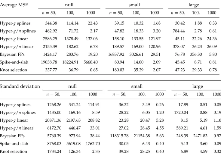
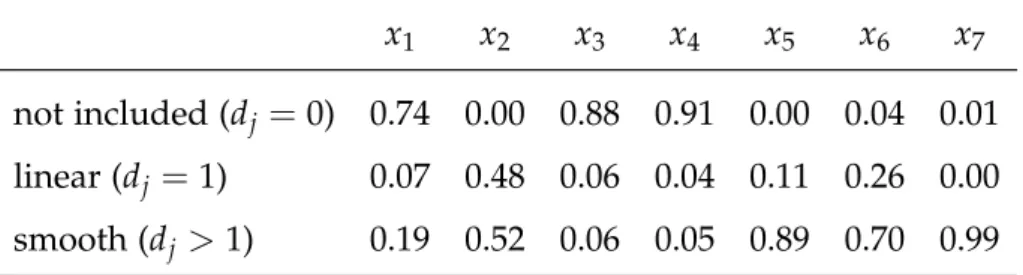
This paper extends the hyper-gpriors to generalised additive models. The additive covariate effects are modelled with penalised splines, represented as mixed models. After integrating out the random effects parametrising the non-linear parts of the splines, the hyper-g prior is applied to the fixed effects parametrising the linear parts. Each additive model is de-fined by the collection of (integer) degrees of freedom for all covariates, which derive from the random effects variances. A suitable objective model prior and a stochastic search algo-rithm are proposed. The methodology is first introduced for models for Gaussian response, and a simulation study demonstrates the advantages over other Bayesian model selection ap-proaches. Consistently with the approach for GLMs, the methodology is extended to models for non-Gaussian response, and illustrated in a logistic regression application. The idea of meta-models differing only in the degrees of freedom of included covariates allows to define intuitive Bayesian model averages.
This work is based on the idea by G. Kauermann to specify the hyper-g prior for the fixed effects in the marginal model, and to discretise the model space by allowing only a finite set of degrees of freedom for the covariate effects. I started the manuscript from the initial draft by G. Kauermann, and generalised his idea to comprise any objective parameter prior for linear models. I implemented the method in the R-package hypergsplines, and wrote a
separateR-packageappellthat calculates Appell’s F1 hypergeometric function that is required
for use of the hyper-g/n prior. L. Held had the idea to extend the objective model prior from variable selection. After G. Kauermann wrote the derivation of the approximate Fisher information for generalised additive models now contained in Appendix B of the paper, I discovered a simpler and more direct explanation based on the iteratively weighted least squares algorithm. I conducted the simulation study on the supercomputer “Schrödinger” and the logistic regression analysis. Both L. Held and G. Kauermann commented on the paper, which I subsequently finalized.
The main contribution of this paper is the idea to apply objective parameter priors developed for linear models to generalised additive models with penalised splines. The implementation with hyper-gpriors shows advantages in a simulation study over competing approaches. Appendix I presents an early version of Paper II which is published in the Proceedings of the 26th International Workshop on Statistical Modelling (2011). This version is less detailed and
Comment on Cai and Betensky (2003), On the Poisson approximation for hazard regression by Daniel Sabanés Bové and Leonhard Held.
This Letter to the Editor contains a correction to the Poisson approximation for proportional hazards regression models proposed by Cai and Betensky (2003, section 5.1) and based on the univariate approach in Cai, Hyndman, and Wand (2002). It is shown that the original approximation, which uses a pseudo data set of the same size nas the original data set, and the resulting log-likelihood has anO(n) error. The correct approximation requires a pseudo
data set that grows withn2.
An extended version is attached. It describes in detail the employed trapezoidal cubature approximation to the cumulative baseline hazard, and slightly improves the original proposal by Cai et al. (2002). It contains an algorithm for computing the required offsets, which also accommodates data sets with ties between the survival times. An application example shows that the error might change the conclusions drawn from the statistical analysis.
The idea for this Letter to the Editor arose from the aim to extend the hyper-g priors from Gaussian, logistic and Poisson regression models covered so far to Cox regression models. After I obtained strange results with the original Poisson approximation, I discovered the error in its derivation and derived the correct approximation. I first drafted the extended version of the manuscript, on which L. Held commented. The Editor of Biometrics then asked for a shortened version suitable for a Letter to the Editor. After L. Held commented on my draft, I finalized it.
The main contribution of this Letter to the Editor is the exposure of the error in the initial publication of the Poisson approximation, and the correction of it, which can be used with a simple R-script written by me. Basically all Cox regression models can be fitted with this
Poisson approximation, which also allows to estimate the baseline hazard.
Paper IV
Approximate Bayesian model selection with the deviance statistic by Daniel Sabanés Bové and Leonhard Held.
This paper merges the hyper-g prior methodology with the test-based Bayes factors (TBFs) proposed by Johnson (2005, 2008). Note that in this paper, the Bayes factor as defined in the Introduction is called data-based Bayes factor, in order to differentiate it from the TBF. It shows that if the deviance statistic is used for the TBFs, the generalized g-prior from Pa-per I is implicitly used. The TBF is a closed form expression in the hyPa-perparameter g, the deviance and the dimension of the model, which allows to conveniently study the influence of g on shrinkage of regression coefficients and model selection. The paper reveals connec-tions of empirical Bayes estimates of g to minimum Bayes factors and shrinkage estimates from the literature. As an alternative, fully Bayes estimation of g is proposed, which effec-tively implements TBF-based hyper-g priors. This approach is especially attractive for large model selection problems because of its computational efficiency, and the corresponding im-plementation issues are discussed in a separate section of the paper. As an example for the development of a clinical prediction model, variable and function selection in a logistic re-gression application is performed with the proposed test-based and the standard data-based
the results are close to those obtained with the Poisson approximation from Paper III.
The initial idea on which this paper is based was from L. Held, who suspected a relation between theg-priors and the TBFs, and proposed to specify a prior distribution forg. I found that the incomplete inverse-gamma prior (Cui and George, 2008) is conjugate to the TBF, and implemented the numerical integration required for non-conjugate hyperpriors. I proved that the generalized g-prior is implicitly assumed in the TBF derivation. I implemented the methodology in theR-packageglmBfp, and conducted all analyses. While