inference for stochastic epidemic models. PhD thesis,
University of Nottingham.
Access from the University of Nottingham repository:
http://eprints.nottingham.ac.uk/29170/1/PhD%20Thesis%20Xiaoguang%20Xu%20ID %204121112%20final.pdf
Copyright and reuse:
The Nottingham ePrints service makes this work by researchers of the University of Nottingham available open access under the following conditions.
· Copyright and all moral rights to the version of the paper presented here belong to the individual author(s) and/or other copyright owners.
· To the extent reasonable and practicable the material made available in Nottingham ePrints has been checked for eligibility before being made available.
· Copies of full items can be used for personal research or study, educational, or not-for-profit purposes without prior permission or charge provided that the authors, title and full bibliographic details are credited, a hyperlink and/or URL is given for the original metadata page and the content is not changed in any way.
· Quotations or similar reproductions must be sufficiently acknowledged. Please see our full end user licence at:
http://eprints.nottingham.ac.uk/end_user_agreement.pdf A note on versions:
The version presented here may differ from the published version or from the version of record. If you wish to cite this item you are advised to consult the publisher’s version. Please see the repository url above for details on accessing the published version and note that access may require a subscription.
for Stochastic Epidemic Models
Xiaoguang Xu
Thesis submitted to The University of Nottingham
for the degree of Doctor of Philosophy
The following errors were discovered after the binding of the printed edition. The corrections are incorporated into the text of the online version only.
p.29. the acceptance ratio is simplified to T×λ∗M×+σ(1g(l′)) should read: the accep-tance ratio is simplified to T×λ∗×Mσ+(−1g(l′))
p.30. the acceptance ratio is simplified to T×λ∗×Mσ(g(l)) should read: the accep-tance ratio is simplified to T×λ∗×Mσ(−g(l))
p.31. ×∏ K k=1σ(g(sk))∏mM=1σ(−g(s˜m))× σ(g(l ′)) σ(g(l)) ×π(g′M+K|{sk}Kk=1,{s˜m}M ′ m=1,θ) ∏Kk=1σ(g(sk))∏Mm=1σ(−g(s˜m))×π(gM+K|{sk}Kk=1,{s˜m}mM=1,θ) should read: × ∏Kk=1σ(g(sk))∏Mm=1σ(−g(s˜m))×σ(−g(l ′)) σ(−g(l)) ×π(g′M+K|{sk}Kk=1,{s˜m}M ′ m=1,θ) ∏Kk=1σ(g(sk))∏Mm=1σ(−g(s˜m))×π(gM+K|{sk}Kk=1,{s˜m}mM=1,θ)
the acceptance ratio is simplified to σσ((gg((ll′)))) should read: the acceptance ratio is simplified to σσ((−−gg((ll′)))) p.38. π(γ|τ,I,I1,h(t))∝ Γ νγ+K,λγ+ Z T I1 γYsds should read: π(γ|τ,I,I1,h(t)) ∝ Γ νγ+K,λγ+ Z T I1 Ysds p.39. ∝ K
∏
j=2 σ(g(Ij−))× K∏
i=1 Yτi− exp − Z T I1 Ysds ×π(gM+K|M,I,{I˜s}Ms=1,θ)∝
∏
j=2 σ(g(Ij−))×∏
i=1 Yτi− exp − I1 γYsds ×π(gM+K|M,I,{I˜s}sM=1,θ) = 1 K−1× T−1I1 ×π(g(Ij−)|Ij,g ′ M+K,I′,{I˜s}Ms=1,T,θ) 1 K−1× T−1I1 ×π(g(I ′ j−)|I′j,gM+K,I,{I˜s}Ms=1,T,θ) ×∏ K j=2σ(−g(I′j−)) ∏Kj=2σ(−g(Ij−)) × ∏ K i=1Yτ′i− exp{− RT I1Y ′ sds} ×π(g′M+K|I′,{I˜s}Ms=1,θ) ∏iK=1Yτi− exp{− RT I1Ysds} ×π(gM+K|I,{ ˜ Is}Ms=1,θ) . should read: = 1 K−1×T−1I1 ×π(g(Ij−)|Ij,g ′ M+K,I′,{I˜s}sM=1,T,θ) 1 K−1×T−1I1 ×π(g(I ′ j−)|Ij′,gM+K,I,{I˜s}sM=1,T,θ) × ∏ K j=2σ(g(Ij′−)) ∏Kj=2σ(g(Ij−)) ×∏ K i=1Yτ′i− exp{− RT I1γY ′ sds} ×π(g′M+K|I′,{I˜s}Ms=1,θ) ∏Ki=1Yτi− exp{− RT I1γYsds} ×π(gM+K|I,{I˜s} M s=1,θ) .p.40. the acceptance ratio is simplified to σ(−g(I′j−)) σ(−g(Ij−)) × ∏iK=1Yτ′ i− exp{− RT I1Y ′ sds} ∏Ki=1Yτi−exp{− RT I1Ysds} .
should read: the acceptance ratio is simplified to σ(g(I′j−)) σ(g(Ij−)) × ∏Ki=1Yτ′ i− exp{− RT I1γY ′ sds} ∏iK=1Yτi− exp{−RTI1γYsds} . p.41. (T−I1)×h∗×σ(g(I˜s′−)) M+1 , and M (T−I1)×β∗×σ(g(I˜s−)) . should read: (T−I1)×h∗×σ(−g(I˜s′−)) M+1 , and M (T−I1)×β∗×σ(−g(I˜s−)) .
Hastings acceptance ratio is σ(−g(Is−)) σ(−g(I˜ s−)) p.62. we have π(γ|τ,I,I1,β(t)) ∝ Γ νγ+K,λγ+ Z T I1 γYsds . should read: we have
π(γ|τ,I,I1,β(t)) ∝ Γ νγ+K,λγ+ Z T I1 Ysds . p.64. π(I,gK|τ,M,{I˜s}sM=1,gM, ˜β∗,γ,T,θ) ∝ K
∏
j=2 XIj−YIj− K∏
j=2 σ(g(Ij−))exp{− Z T I1 XsYsds} × K∏
i=1 Yτi− exp{− Z T I1 Ysds} ×π(gM+K|M,I,{I˜s}Ms=1,θ). should read: π(I,gK|τ,M,{I˜s}sM=1,gM, ˜β∗,γ,T,θ) ∝ K∏
j=2 XI j−YIj− K∏
j=2 σ(g(Ij−))exp{− Z T I1 ˜ β∗XsYsds} × K∏
i=1 Yτi− exp{− Z T I1 γYsds} ×π(gM+K|M,I,{I˜s}Ms=1,θ). p.65. × ∏Kj=2X′I j−Y ′ Ij− ×∏Kj=2σ(−g(Ij′))exp{− RT I1X ′ sYs′ds} ∏Kj=2XIj−YIj− ∏Kj=2σ(−g(Ij))exp{−RTI1XsYsds} ×∏ K i=1Yτ′i− exp{− RT I1Y ′ sds} ×π(g′M+K|{Ij′}Kj=2,{I˜s}Ms=1,θ) ∏Ki=1Yτi− exp{−RTI1Ysds} ×π(gM+K|I,{I˜s}sM=1,θ) . should read: × ∏Kj=2X′I j−Y ′ Ij− ×∏Kj=2σ(g(I′j))exp{− RT I1 ˜ β∗Xs′Ys′ds} ∏Kj=2XIj−YIj− ∏ K j=2σ(g(Ij))exp{− RT I1 ˜ β∗XsYsds} × ∏ K i=1Yτ′i− exp{− RT I1γY ′ sds} ×π(g′M+K|{I′j}Kj=2,{I˜s}Ms=1,θ) ∏Ki=1Yτi− exp{− RT I1γYsds} ×π(gM+K|I,{ ˜ Is}sM=1,θ) .∏j=2XI j−YIj− ×σ(−g(Ij))exp{− I1XsYsds} ∏Kj=2XI j−YIj−σ(−g(Ij))exp{− RT I1XsYsds} ×∏ K i=1Yτ′i− exp{− I1Y ′ sds} ∏iK=1Yτi− exp{−RTI1Ysds} .
should read: the acceptance ratio is simplified to
∏Kj=2X′I j−Y ′ Ij− ×σ(g(Ij′))exp{− RT I1 ˜ β∗X′sYs′ds} ∏Kj=2XIj−YIj−σ(g(Ij))exp{− RT I1 ˜ β∗XsYsds} ×∏ K i=1Yτ′i− exp{− RT I1γY ′ sds} ∏Ki=1Yτi− exp{− RT I1γYsds} .
p.66. The acceptance ratio is
q(M′→M) q(M→M′) × π(M′,{I˜s}mM=′1,g′M|I,gK,θ, ˜β∗) π(M,{I˜s}sM=1,gM|I,gK,θ, ˜β∗) = 1 2 ×M1′ 1 2× T−1I1 ×π(g(I˜ ′ s−)|I˜s′,gM+K,I,{I˜s}Ms=1,θ) × ( ˜ β∗)M′∏sM=′1XI˜ s−YI˜s−∏ M′ m=1σ(−g(I˜s−))×π(gM′ +K|I,{I˜s}Mm=′ 1,θ) (β˜∗)M∏M s=1XI˜s−YI˜s− ∏mM=1σ(−g(I˜s−))×π(gM+K|I,{I˜s}sM=1,θ) . should read: The acceptance ratio is
q(M′→M) q(M→M′) × π(M′,{I˜s}sM=′1,g′M|I,gK,θ, ˜β∗) π(M,{I˜s}Ms=1,gM|I,gK,θ, ˜β∗) = 1 2×M1′ 1 2 ×T−1I1 ×π(g( ˜ Is′−)|I˜′ s,gM+K,I,{I˜s}sM=1,θ) × ( ˜ β∗)M′∏Ms=′1XI˜ s−YI˜s− ∏ M′ s=1σ(−g(I˜s−))×π(gM′ +K|I,{I˜s}Ms=′1,θ) (β˜∗)M∏M s=1XI˜s−YI˜s− ∏Ms=1σ(−g(I˜s−))×π(gM+K|I,{I˜s}Ms=1,θ) . p.67. π(g′M+K|I,{I˜s}mM=′1,θ) =π(gM+K|I,{I˜s}sM=1,θ)×π(g(I˜s′−)|I˜s′,gM+K,I,{I˜s}Ms=1,θ),
the acceptance ratio is simplified to
(T−I1)×β˜∗×σ(g(I˜s′−))×XI˜′ s− Y˜I′ s− M+1 should read: π(g′M+K|I,{I˜s}sM=′1,θ) =π(gM+K|I,{I˜s}sM=1,θ)×π(g(I˜s′−)|I˜s′,gM+K,I,{I˜s}Ms=1,θ),
the acceptance ratio is simplified to
(T−I1)×β˜∗×σ(−g(I˜s′−))×XI˜′
s−
YI˜′
s−
should read: q(M′→M) = 1 2 × 1 T−I1 × π(g(I˜s−)|I˜s,g′M+K,I,{I˜s}sM=′1,θ).
The acceptance ratio is
q(M′→M) q(M→M′) × π(M′,{I˜s}mM=′1,g′M|I,{I˜s}sM=1,gK,θ, ˜β∗) π(M,{I˜s}sM=1,gM|I,{I˜s}sM=′1,gK,θ, ˜β∗) = 1 2× T−1I1 ×π(g(I˜s−)|I˜s,g ′ M+K,I,{I˜s}M ′ m=1,θ) 1 2× M1 × ( ˜ β∗)M′∏M′ s=1XI˜s−YI˜s−∏ M′ m=1σ(−g(I˜s−))×π(gM′ +K|I,{I˜s}Mm=′ 1,θ) (β˜∗)M∏M s=1XI˜s−YI˜s− ∏ M m=1σ(−g(I˜s−))×π(gM+K|I,{I˜s}sM=1,θ) . should read: The acceptance ratio is
q(M′→M) q(M→M′) × π(M′,{I˜s}sM=′1,g′M|I,{I˜s}sM=1,gK,θ, ˜β∗) π(M,{I˜s}Ms=1,gM|I,{I˜s}Ms=′1,gK,θ, ˜β∗) = 1 2 ×T−1I1 ×π(g(I˜s−)|I˜s,g ′ M+K,I,{I˜s}M ′ s=1,θ) 1 2 ×M1 × ( ˜ β∗)M′∏M′ s=1XI˜s−YI˜s− ∏Ms=′1σ(−g(I˜s−))×π(g′M+K|I,{I˜s}Ms=′1,θ) (β˜∗)M∏M s=1XI˜s−YI˜s− ∏Ms=1σ(−g(I˜s−))×π(gM+K|I,{I˜s}Ms=1,θ) . =π(g′M+K|I,{I˜s}mM=′1,θ)×π(g(I˜s−)|I˜s,g′M+K,I,{I˜s}mM=′1,θ),
the acceptance ratio is simplified to ( M
T−I1)×β˜∗×σ(g(I˜s−))×XI˜s−Y˜Is− should read:
=π(g′M+K|I,{I˜s}Ms=′1,θ)×π(g(I˜s−)|I˜s,g′M+K,I,{I˜s}sM=′1,θ),
the acceptance ratio is simplified to ( M
T−I1)×β˜∗×σ(−g(I˜s−))×XI˜s−YI˜s− p.68. × ∏sM=−11XI˜ s−YI˜s− × XI˜′ s−YI˜′s− XI˜s−YI˜s− ∏ M m=1σ(−g(I˜s))×σ(g( ˜ Is′)) σ(g(I˜s)) ×π(g′M+K|I,{I˜s}sM=′1,θ) ∏sM=−11XI˜ s−YI˜s− ∏ M m=1σ(−g(I˜s))×π(gM+K|I,{I˜s}sM=1,θ) .
× ∏sM=−11XI˜ s−YI˜s− × s− s− XI˜ s−YI˜s− ∏Ms=1σ(−g(I˜s))×σσ((−−gg((II˜ss)))) ×π(g′M+K|I,{I˜s}sM=1,θ) ∏sM=−11XI˜ s−YI˜s− ∏ M s=1σ(−g(I˜s))×π(gM+K|I,{I˜s}Ms=1,θ) .
the acceptance ratio is simplified to XI˜′
s−
YI˜′
s−×
σ(g(I˜s′−))
XI˜s−YI˜s−×σ(g(I˜s−)) should read: the
accep-tance ratio is simplified to XI˜′ s−YI˜s′−×σ (−g(I˜′ s−)) XI˜ s−YI˜s−×σ(−g( ˜ Is−)) p.89. π(γ|βββ˜(t),τττ,I e) ∝ Γ νγ+ k
∑
i=1 ni,λγ+ k∑
i=1 Z T Ii1 γYi(s)ds ! . should read: π(γ|βββ˜(t),τττ,I e) ∝ Γ νγ+ k∑
i=1 ni,λγ+ k∑
i=1 Z T Ii1 Yi(s)ds ! .Modelling of infectious diseases is a topic of great importance. Despite the enormous attention given to the development of methods for efficient parame-ter estimation, there has been relatively little activity in the area of nonparamet-ric inference for epidemics. In this thesis, we develop new methodology which enables nonparametric estimation of the parameters which govern transmis-sion within a Bayesian framework. Many standard modelling and data analy-sis methods use underlying assumptions (e.g. concerning the rate at which new cases of disease will occur) which are rarely challenged or tested in practice. we relax these assumptions and analyse data from disease outbreaks in a Bayesian nonparametric framework.
We first apply our Bayesian nonparametric methods to small-scale epidemics. In a standard SIR model, the overall force of infection is assumed to have a parametric form. We relax this assumption and treat it as a function which only depends on time. Then we place a Gaussian process prior on it and infer it using data-augmented Markov Chain Monte Carlo (MCMC) algorithms. Our methods are illustrated by applications to simulated data as well as Smallpox data. We also investigate the infection rate in the SIR model using our methods. More precisely, we assume the infection rate is time-varying and place a Gaus-sian process prior on it. Results are obtained using data augmentation methods and standard MCMC algorithms. We illustrate our methods using simulated data and respiratory disease data. We find our methods work fairly well for the stochastic SIR model.
We also investigate large-scaled epidemics in a Bayesian nonparametric frame-work. For large epidemics in large populations, we usually observe surveil-lance data which typically provide number of new infection cases occurring during observation periods. We infer the infection rate for each observation
pe-I feel very fortunate to have Philip O’Neill and Theodore Kypraios as my su-pervisors. They were always there for me and I am very grateful for all their guidance, advice and patience during my PhD studies.
Many thanks to my parents for all their support and patience.
I would also like to thank my friends in Nottingham for making my life more enjoyable.
Many thanks to the University of Nottingham School of Mathematical Sciences who fully funded my PhD study.
Finally, there is nothing I could do to sufficiently express my gratitude to Lin. She has been very supportive and understanding.
List of Figures VIII
List of Tables XXVII
1 Introduction 1
1.1 Motivation . . . 1
1.2 Bayesian inference . . . 3
1.2.1 Bayes’ theorem . . . 3
1.2.2 Markov Chain Monte Carlo . . . 4
1.2.2.1 The Metropolis-Hastings algorithm . . . 4
1.2.2.2 Gibbs sampler . . . 5
1.2.2.3 Burn-in . . . 6
1.2.2.4 Thinning . . . 6
1.2.2.5 Proposal distributions and convergence . . . 6
1.3 Epidemic modelling . . . 7
1.3.1 Stochastic SIR model . . . 7
1.3.2 Bayesian inference for the SIR model from partially ob-served data . . . 9
1.4 Bayesian nonparametric model . . . 10
1.5 Gaussian process . . . 12
1.5.1 Introduction . . . 12
1.5.3 Covariance function . . . 13
1.5.4 Gaussian process prediction . . . 17
1.6 Overview. . . 19
2 Bayesian nonparametric estimation for the overall force of infection in small-scale epidemics 21 2.1 Introduction . . . 21
2.2 Estimation for inhomogeneous Poisson process . . . 23
2.2.1 Introduction . . . 23
2.2.2 Sigmoidal Gaussian Cox process model . . . 23
2.2.3 Generating exact Poisson data . . . 24
2.2.4 Inference . . . 25
2.2.4.1 Doubly intractable problem . . . 25
2.2.5 Data augmentation . . . 27
2.2.6 MCMC sampling . . . 28
2.2.7 Simulated Poisson data study . . . 33
2.3 Estimation for epidemic models . . . 36
2.3.1 MCMC algorithms . . . 38
2.3.2 Simulated complete data. . . 42
2.3.3 Simulated partial data . . . 45
2.3.4 Smallpox data . . . 48
2.4 Sensitivity to the Gaussian process prior for the SIR epidemic model . . . 53
2.5 Conclusion . . . 57
3 Bayesian nonparametric estimation for the infection rate in small-scale epidemics 59 3.1 Introduction . . . 59
3.2.1 Inference . . . 61
3.2.1.1 MCMC algorithms. . . 63
3.2.2 Simulated complete single group data . . . 69
3.2.2.1 Constant infection rate . . . 69
3.2.2.2 Infection rate varies throughout the epidemic . . 72
3.2.3 Simulated partially observed single group data . . . 74
3.2.3.1 Constant infection rate . . . 74
3.2.3.2 Infection rate varies throughout the epidemic . . 74
3.2.4 Smallpox data . . . 80
3.3 Sensitivity to the Gaussian process prior for the SIR epidemic model . . . 82
3.4 Estimation for epidemic models from multi-group epidemic data 86 3.4.1 Multi-group epidemic model . . . 86
3.4.2 Inference . . . 87
3.4.3 Simulated partially observed multi-group data . . . 90
3.4.4 Respiratory disease multi-group data . . . 93
3.5 Comparison withh(t)approach . . . 97
3.6 Conclusion . . . 100
4 Bayesian nonparametric estimation for epidemic models in large pop-ulations from time-series data 102 4.1 Introduction . . . 102
4.2 Approximation to the SIR epidemic model . . . 103
4.2.1 Introduction . . . 103
4.2.2 The Cox-Ingersoll-Ross diffusion process . . . 106
4.3 Inference . . . 110
4.3.1 MCMC sampling . . . 111
4.3.1.2 Sampling the infection rates . . . 111
4.3.1.3 Sampling the total number of new infections . . 112
4.3.1.4 Sampling the initial number of susceptibles . . . 113
4.3.1.5 Sampling the number of infectives . . . 113
4.4 Simulation study using Cauchemez & Ferguson’s method . . . . 114
4.5 Bayesian nonparametric estimation on infection rates . . . 116
4.5.1 Seasonal assumption on infection rates . . . 118
4.5.1.1 Sampling the function values . . . 119
4.5.1.2 Sampling the hyperparameters . . . 119
4.5.1.3 Results . . . 120
4.5.2 Seasonal assumption on infection rates relaxed . . . 120
4.5.3 Different parameter settings for the Gaussian process . . . 124
4.5.3.1 Strong prior on hyperparameters for Gaussian processes . . . 124
4.5.3.2 Different covariance functions for Gaussian pro-cesses . . . 125
4.6 Measles epidemics in london (1948-1957) . . . 128
4.7 Conclusion . . . 130
5 Conclusions 135
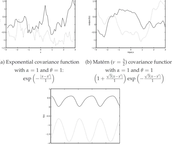
1.1 Samples drawn from Gaussian process priors. The figure shows two functions (solid and dotted) drawn from each of three Gaus-sian process priors with the squared exponential covariance func-tion. The sample functions are obtained using a discretization of thex-axis of 60 equally spaced points. The corresponding covari-ance function is given below each plot. . . 16 1.2 Samples drawn from Gaussian process priors. The figure shows
two functions (solid and dotted) drawn from each of six Gaus-sian process priors with different covariance functions. The func-tions are obtained using a discretization of the x-axis of 60 and 100 equally spaced points for plots (a) and (b) and plot (f) re-spectively. The corresponding covariance function is given be-low each plot. . . 17 1.3 5 random samples are generated from the GP with the same
co-variance function, the squared exponential coco-variance function, where the hyperparameters α = 1 and θ = 1. The samples are obtained using a discretization of thex-axis of 60 equally spaced points. . . 18 1.4 Given three observations (-1.15,0), (0.15,-1), (1.15,0), 5 random
samples are generated from the Gaussian process with the same covariance function, the squared exponential covariance func-tion, where the hyperparameters α = 1 and θ = 1. The sam-ples are obtained using a discretization of thex-axis of 60 equally spaced points. . . 19
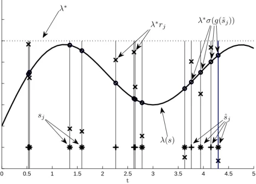
2.1 Procedure for generating exact Poisson data via a thinning method. A Poisson time series,{sˆj}jJ=1(+and∗marks), is generated from a homogeneous Poisson process with rate, λ∗. At each point of the time series, a sample,g(sˆj), is drawn from the Gaussian
pro-cess. Then the function value is transformed through the sigmoid function so that it is in form ofλ∗σ(g(sˆj)) (◦ marks) and is pos-itive and bounded above by λ∗. Variates, {λ∗rj}Jj=1 (×marks), are drawn uniformly on (0,λ) in the vertical coordinate. If the variates are greater than the transformed function values, the corresponding events are discarded (+ marks). The remaining events,{sj}Jj=1(∗marks), are the exact Poisson events generated from the inhomogeneous Poisson process corresponding to the random function,λ(s). . . 26 2.2 Plot (a) shows posterior mean of the inhomogeneous Poisson
process intensity λ(t) at each Poisson point compared with the true λ(t) generated from a transformed Gaussian process (see (2.1)) given by λ∗ = 60, T = 7 and a zero mean and a value of hyperparameter,θ = 1.5, for the Gaussian process. The Poisson data are shown by “ | ” marks. The 95% credible intervals are shown as well. Plot (b) shows the MCMC trace plot of the hyper-parameter θ compared with the true θ (dotted line) for the first Poisson data set. . . 34 2.3 Plot (a) shows posterior mean of the inhomogeneous Poisson
process intensity λ(t) at each Poisson point compared with the true λ(t) generated from a transformed Gaussian process given by λ∗ = 60, T = 7 and a zero mean and a value of hyperpa-rameter, θ = 1.5, for the Gaussian process. The Poisson data are shown by “ |” marks. The 95% credible intervals are shown as well. Plot 2.3 (b) shows the MCMC trace plot of the hyperpa-rameter θ compared with the true θ (dotted line) for the second Poisson data set. . . 34
2.4 Plot (a) shows posterior mean of the inhomogeneous Poisson process intensity λ(t) at each Poisson point compared with the true λ(t) generated from a transformed Gaussian process given by λ∗ = 40, T = 5 and a zero mean and a value of hyperpa-rameter, θ = 1.5, for the Gaussian process. The Poisson data are shown by “ |” marks. The 95% credible intervals are shown as well. Plot 2.4 (b) shows the MCMC trace plot the hyperparame-terθ compared with the trueθ (dotted line) for the third Poisson data set.. . . 35 2.5 Posterior mean of the inhomogeneous Poisson process intensity
λ(t) at each Poisson point compared with the truth λ(t) = 10 (dotted line). The Poisson data (“|” marks) are generated from the intensityλ(t) = 10 within a time region[0, 10]. . . 35 2.6 Posterior mean of the inhomogeneous Poisson process intensity
λ(t) at each Poisson point compared with the truth λ(t) = 10 (dotted line). The Poisson data, different from the one in Figure 2.5, (“|” marks) are generated with the same parameter setting, i.e. from the intensityλ(t) =10 within a time region[0, 10]. . . . 36 2.7 Posterior mean of the overall force of infectionh(t) (solid line) at
each infection time compared with the original dataβXtYt
(dot-ted line) genera(dot-ted from the general stochastic epidemic with pa-rameters infection rate β = 0.025, removal rate γ = 1, initial number of susceptibles N = 100 and initial number of infective individualsa =1. The 95% credible intervals are shown as well. There is a total of 87 infections during the whole epidemic and all the infection times are assumed to be known. The “|” marks in the plot represent the observed data, i.e. the infection times. The squared exponential covariance function is used for the Gaussian process prior and the hyperparameter of the covariance function, α, is set to 2. . . 44
2.8 Posterior mean of the overall force of infectionh(t) (solid line) at each infection time compared with the original dataβXtYt
(dot-ted line) genera(dot-ted from the general stochastic epidemic with pa-rameters infection rate β = 0.015, removal rate γ = 1, initial number of susceptibles N = 150 and initial number of infec-tive individuals a = 1. The 95% credible intervals are shown as well. There is a total of 130 infections during the whole epi-demic and all the infection times are assumed to be known. The “|” marks in the plot represent the observed data, i.e. the infec-tion times. The squared exponential covariance funcinfec-tion is used for the Gaussian process prior and the hyperparameter of the co-variance function,α, is set to 2. . . 44 2.9 Posterior mean of the overall force of infectionh(t) (solid line) at
each infection time compared with the original dataβXtYt
(dot-ted line) genera(dot-ted from the general stochastic epidemic with pa-rameters infection rate β = 0.015, removal rate γ = 1, initial number of susceptibles N = 200 and initial number of infec-tive individuals a = 1. The 95% credible intervals are shown as well. There is a total of 189 infections during the whole epi-demic and all the infection times are assumed to be known. The “|” marks in the plot represent the observed data, i.e. the
infec-tion times. The squared exponential covariance funcinfec-tion is used for the Gaussian process prior and the hyperparameter of the co-variance function,α, is set to 2. . . 45
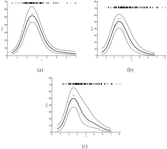
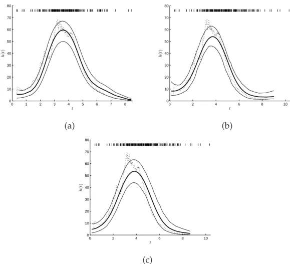
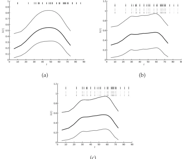
2.10 Dataset SE-Data 2 recovered by placing the Gaussian process prior. Three plots show posterior mean of the overall force of infection h(t) (solid line) at each infection time compared with the original data βXtYt (dotted line) generated from the general
stochastic epidemic with parameters β =0.015, γ =1, N =150 and a =1. Plot (a) corresponds to the case where complete data are observed. Plot (b) corresponds to the case where removal times are known as well as the removal rate. Plot (c) corresponds to the case where only removal times are known. The 95% cred-ible intervals are shown for each of the plot. The “ | ” marks in each plot represent the observed data, i.e. the infection times for plot (a) and the removal times for plot (b) and (c). There is a total of 130 infections during the whole epidemic. The squared exponential covariance function is used for the Gaussian process prior and the hyperparameter of the covariance function,α, is set to 2. . . 47 2.11 Dataset SE-Data 2 recovered by placing the Gaussian process
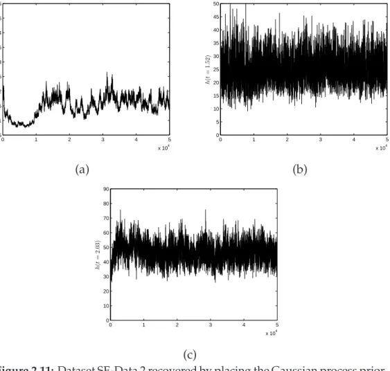
prior where only removal times are known. Plot (a) shows MCMC trace plot of the hyperparameter,θ. Plot (b) and (c) show MCMC trace plot of the overall force of infection at time t = 1.52 and t = 2.03 respectively. The squared exponential covariance func-tion is used for the Gaussian process prior and the hyperparam-eter of the covariance function, α, is set to 2. . . 48
2.12 Dataset SE-Data 3 recovered by placing the Gaussian process prior. Three plots show posterior mean of the overall force of infection h(t) (solid line) at each infection time compared with the original data βXtYt (dotted line) generated from the general
stochastic epidemic with parameters β =0.015, γ =1, N =200 anda =1. Plot (a) corresponds to the case where infection times are known. Plot (b) corresponds to the case where removal times are known as well as the removal rate. Plot (c) corresponds to the case where only removal times are known. The 95% cred-ible intervals are shown for each of the plot. The “ | ” marks in each plot represent the observed data, i.e. the infection times for plot (a) and the removal times for plot (b) and (c). There is a total of 189 infections during the whole epidemic. The squared exponential covariance function is used for the Gaussian process prior and the hyperparameter of the covariance function,α, is set to 2. . . 49 2.13 Posterior mean of force of infection h(t) (solid line) at each
esti-mated infection time. The 95% credible intervals are shown as well. There is a total of 30 infections during the whole epidemic and all the infection times and the removal rate are assumed to be unknown. Only removal times are known. The “|” marks in
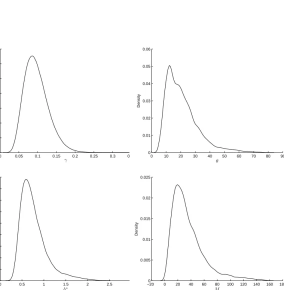
the plot represent the observed data, i.e. the removal times. The squared exponential covariance function is used for the Gaussian process prior and the hyperparameter of the covariance function, α, is set to 2. . . 51 2.14 Densities of removal rate,γ, hyperparameter,θ, upper boundh∗
2.15 Posterior mean of the infection rate, ˆβ(t) at each estimated in-fection time for the Smallpox data. The 95% credible intervals are shown as well. There is a total of 30 infections during the whole epidemic and all the infection times and the removal rate are assumed to be unknown. Only removal times are known. The “ |” marks in the plot represent the observed data, i.e. the removal times. The squared exponential covariance function is used for the Gaussian process prior and the hyperparameter of the covariance function,α, is set to 2. . . 53 2.16 Dataset SE-Data 2 recovered by placing three different Gaussian
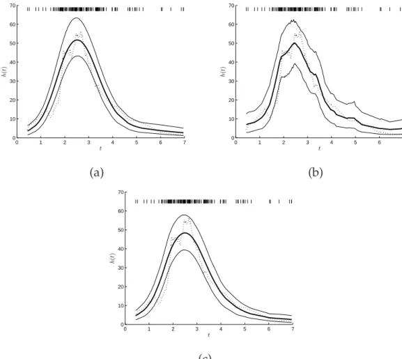
process priors. Three plots show posterior mean of the overall force of infection h(t) (solid line) at each infection time com-pared with the original data βXtYt (dotted line) generated from
the general stochastic epidemic with parameters infection rate β = 0.015, removal rate γ = 1, initial number of susceptibles N = 200 and initial number of infective individuals a = 1. Plot (a) corresponds to the squared exponential covariance function see, (1.2). Plot (b) corresponds to the exponential covariance function see, (1.3). Plot (c) corresponds to the Matérn covariance function with ν set to 3/2 see, (1.4). The 95% credible intervals are shown for each of the plot. The “|” marks in each plot
rep-resent the observed data, i.e. the infection times. There is a total of 130 infections during the whole epidemic and all the infection times are assumed to be known. The hyperparameter of the three covariance functions,α, is set to 2. . . 55 2.17 Dataset SE-Data 2 recovered by placing three different Gaussian
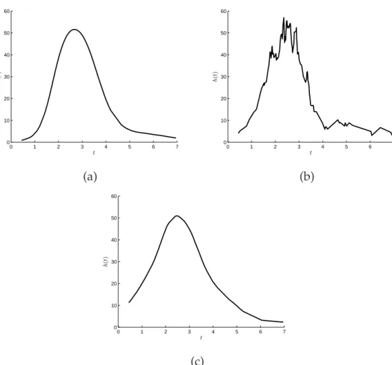
process priors. Three plots show posterior samples of the overall force of infectionh(t) (solid line) at each infection time. Plot (a) corresponds to the squared exponential covariance function see, (1.2). Plot (b) corresponds to the exponential covariance function see, (1.3). Plot (c) corresponds to the Matérn covariance function with νset to 3/2 see, (1.4). The hyperparameter of the three co-variance functions,α, is set to 2. . . 56
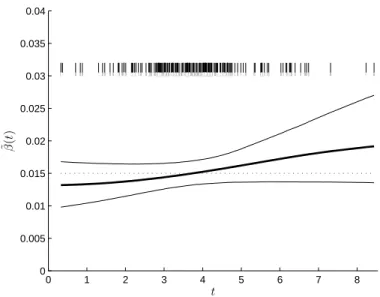
2.18 Smallpox recovered by placing three different Gaussian process priors. Plot (a) corresponds to the squared exponential covari-ance function see, (1.2). Plot (b) corresponds to the exponential covariance function see, (1.3). Plot (c) corresponds to the Matérn covariance function with ν set to 3/2 see, (1.4). The 95% cred-ible intervals are shown for each of the plot. The “ | ” marks in each plot represent the observed data, i.e. the removal times. There is a total of 30 infections during the whole epidemic and only removal times are known. The hyperparameter of the three covariance functions,α, is set to 2. . . 57 3.1 Posterior mean of the infection rate ˜β(t)(solid line) at each
infec-tion time for SE-Data 1. The 95% credible intervals are shown as well. True infection rate (dotted line), β =0.025. There is a total of 87 infections during the whole epidemic and all the infection times are assumed to be known. The “|” marks in the plot rep-resent the observed data, i.e. the infection times. The squared exponential covariance function is used for the Gaussian process prior and the hyperparameter of the covariance function, α, is fixed to 1. . . 70 3.2 Posterior mean of the infection rate ˜β(t)(solid line) at each
infec-tion time for SE-Data 2. The 95% credible intervals are shown as well. True infection rate (dotted line), β =0.015. There is a total of 130 infections during the whole epidemic and all the infection times are assumed to be known. The “|” marks in the plot rep-resent the observed data, i.e. the infection times. The squared exponential covariance function is used for the Gaussian process prior and the hyperparameter of the covariance function, α, is fixed to 1. . . 71
3.3 Posterior mean of the infection rate ˜β(t)(solid line) at each infec-tion time for SE-Data 3. The 95% credible intervals are shown as well. True infection rate (dotted line), β =0.015. There is a total of 189 infections during the whole epidemic and all the infection times are assumed to be known. The “|” marks in the plot rep-resent the observed data, i.e. the infection times. The squared exponential covariance function is used for the Gaussian process prior and the hyperparameter of the covariance function, α, is fixed to 1. . . 72 3.4 Posterior mean of the infection rate ˜β(t) (solid line) at each
in-fection time compared with true inin-fection rate (dotted line). The 95% credible intervals are shown as well. There is a total of 222 infections during the whole epidemic and all the infection times are assumed to be known. The “| ” marks in the plot represent the observed data, i.e. the infection times. The squared exponen-tial covariance function is used for the Gaussian process prior and the hyperparameter of the covariance function,α, is fixed to 1. 73 3.5 Posterior mean of the infection rate ˜β(t) (solid line) at each
esti-mated infection time for SE-Data 1 (plot (a) and plot(b)). True in-fection rate (dotted line),β=0.025 and true removal rate,γ=1. The 95% credible intervals are shown in (a) and (b). Plot (a) is the case where complete data are observed. Plot (b) is the case where only removal times are observed. The “|” marks in each plot represent the observed data, i.e. the infection times in (a) and removal times in (b). Plot (c) shows density of the removal rate for the second case. There is a total of 87 infections during the whole epidemic. The squared exponential covariance function is used for the Gaussian process prior and the hyperparameter of the covariance function,α, is fixed to 1.. . . 75
3.6 Posterior mean of the infection rate ˜β(t) (solid line) at each esti-mated infection time for SE-Data 2 (plot (a) and plot(b)). True in-fection rate (dotted line),β=0.015 and true removal rate,γ=1. The 95% credible intervals are shown in (a) and (b). Plot (a) is the case where complete data are observed. Plot (b) is the case where only removal times are observed. The “|” marks in each plot represent the observed data, i.e. the infection times in (a) and removal times in (b). Plot (c) shows density of the removal rate for the second case. There is a total of 130 infections during the whole epidemic. The squared exponential covariance function is used for the Gaussian process prior and the hyperparameter of the covariance function,α, is fixed to 1.. . . 76 3.7 Dataset SE-Data 2 recovered by placing the Gaussian process
prior where only removal times are known. Plot (a) shows MCMC trace plot of the hyperparameter,θ. Plot (b) and (c) show MCMC trace plot of the infection rate at time t = 2.42 and t = 3.42 re-spectively. The squared exponential covariance function is used for the Gaussian process prior and the hyperparameter of the co-variance function,α, is fixed to 1. . . 77 3.8 Posterior mean of the infection rate ˜β(t) (solid line) at each
esti-mated infection time for SE-Data 3 (plot (a) and plot(b)). True in-fection rate (dotted line),β=0.015 and true removal rate,γ=1. The 95% credible intervals are shown in (a) and (b). Plot (a) is the case where complete data are observed. Plot (b) is the case where only removal times are observed. The “|” marks in each
plot represent the observed data, i.e. the infection times in (a) and removal times in (b). Plot (c) shows density of the removal rate for the second case. There is a total of 189 infections during the whole epidemic. The squared exponential covariance function is used for the Gaussian process prior and the hyperparameter of the covariance function,α, is fixed to 1.. . . 78
3.9 Posterior mean of the infection rate ˜β(t) (solid line) at each esti-mated infection time for SE-Data 4 (plot (a) and plot (b)). True removal rate, γ = 0.7. The 95% credible intervals are shown in (a) and (b). Plot (a) is the case where complete data are observed. Plot (b) is the case where only removal times are observed. The “
|” marks in each plot represent the observed data, i.e. the infec-tion times in (a) and removal times in (b). Plot (c) shows density of the removal rate for the second case. There is a total of 222 infections during the whole epidemic. The squared exponential covariance function is used for the Gaussian process prior and the hyperparameter of the covariance function,α, is fixed to 1. . . 79 3.10 Smallpox data recovered by placing the Gaussian process prior.
The plot (a) shows posterior mean of the infection rate, ˜β(t), at each estimated infection time using our Bayesian nonparamet-ric methods where the squared exponential covariance function is adopted. The “ | ” marks in the plot represent the observed
data, i.e. the removal times. The plot (b), obtained from Becker (1989), p.137, shows two estimation results of the infection rate for smallpox data from Becker’s methods. The infection rate is assumed to be a decreasing function of time in the two models. . 81 3.11 Smallpox data recovered by placing the Gaussian process prior
on ˜β(t). Four plots show densities of the removal rate,γ, the hy-perparameter,θ, the upper bound ˜β∗ and the number of thinned events,Mrespectively. The squared exponential covariance func-tion for the Gaussian process prior is adopted. . . 82
3.12 Dataset SE-Data 2 recovered by placing three different Gaussian process priors. Three plots show posterior mean of the infec-tion rate, ˜β(t) (solid line) at each infection time compared with the trueβ(dotted line). The data are generated from the general stochastic epidemic with parameters infection rate β=0.015, re-moval rateγ =1, initial number of susceptiblesN =150 and ini-tial number of infective individuals a = 1. Plot (a) corresponds to the squared exponential covariance function see, (1.2). Plot (b) corresponds to the exponential covariance function see, (1.3). Plot (c) corresponds to the Matérn covariance function withνset to 3/2 see, (1.4). The 95% credible intervals are shown for each of the plot. The “|” marks in each plot represent the observed data,
i.e. the infection times. There is a total of 130 infections during the whole epidemic and all the infection times are assumed to be known. The hyperparameter of the three covariance functions, α, is set to 1. . . 84 3.13 Smallpox recovered by placing three different Gaussian process
priors. Three plots show posterior mean of the infection rate, ˜β(t)
(solid line) at each estimated infection time. Plot (a) corresponds to the squared exponential covariance function see, (1.2). Plot (b) corresponds to the exponential covariance function see, (1.3). Plot (c) corresponds to the Matérn covariance function withνset to 3/2 see, (1.4). The 95% credible intervals are shown for each of the plot. The “ |” marks in each plot represent the observed data, i.e. the removal times. There is a total of 30 infections dur-ing the whole epidemic and only removal times are known. The hyperparameter of the three covariance functions,α, is set to 1.. . 85
3.14 (a), posterior mean of the infection rate ˜β1(t) (solid line) at each estimated infection time for SE-Data 5. True infection rate,β1 =
0.005. The 95% credible intervals are shown as well. (b), poste-rior mean of the infection rate ˜β2(t)(solid line) at each estimated
infection time for SE-Data 5. True infection rate, β2 =0.005. The
95% credible intervals are shown as well. Only removal times of each group are known. The “|” marks in each plot represent the
observed data, i.e. the removal times. The squared exponential covariance function is used for the Gaussian process prior and the hyperparameter,α, is fixed to 1. . . 92 3.15 (a), posterior mean of the infection rate ˜β3(t) (solid line) at each
estimated infection time for SE-Data 5. True infection rate, β =
0.002 and true removal rate, γ = 0.5. The 95% credible intervals are shown as well. (b), density of the removal rate. Only removal times of each group are known. The “|” marks in the plot
rep-resent the observed data, i.e. the removal times. The squared exponential covariance function is used for the Gaussian process prior and the hyperparameter of the covariance function, α, is fixed to 1. . . 94 3.16 (a), posterior mean of the infection rate ˜βinfants(t) (solid line) at
each estimated infection time for the respiratory disease data (Hayakawa et al., 2003). The 95% credible intervals are shown as well. (b), posterior mean of the infection rate ˜βchildren(t)(solid line) at each estimated infection time for the respiratory disease data. The 95% credible intervals are shown as well. Only re-moval times of each group are known. The “| ” marks in each
plot represent the observed data, i.e. the removal times. The squared exponential covariance function is used for the Gaussian process prior and the hyperparameter of the covariance function, α, is fixed to 1. . . 95
3.17 (a), posterior mean of the infection rate ˜βadults(t) (solid line) at each estimated infection time for the respiratory disease data (Hayakawa et al., 2003). The 95% credible intervals are shown as well. (b), density of the removal rate. Only removal times in each group are known. The “|” marks in the plot represent the observed data, i.e. the removal times. The squared exponential covariance function is used for the Gaussian process prior and the hyperparameter of the covariance function,α, is fixed to 1. . . 96 3.18 Dataset SE-Data 2 recovered by placing the Gaussian process
prior with different Bayesian nonparametric methods. Two plots show posterior mean of the infection rate, ˆβ(t) and ˜β(t) (solid line) at each infection time respectively. The original data βXtYt
(dotted line) are generated from the general stochastic epidemic with parameters infection rate β = 0.015, removal rate γ = 1, initial number of susceptibles N = 150 and initial number of infective individuals a = 1. Only removal times are observed for both cases. Plot (a) corresponds to the case where the ap-proach discussed in Chapter 2 is used. Plot (b) corresponds to the case where the approach discussed in Chapter 3 is used. The 95% credible intervals are shown for each of the plot. The “ |” marks in each plot represent the observed data, i.e. the removal times. The squared exponential covariance function is used for the Gaussian process prior and the hyperparameter of the covari-ance function,α, is set to 2 and 1 for ˆβ(t)and ˜β(t) respectively. . . 98
3.19 Dataset SE-Data 3 recovered by placing the Gaussian process prior with different Bayesian nonparametric methods. Two plots show posterior mean of the infection rate, ˆβ(t) and ˜β(t) (solid line) at each infection time respectively. The original data βXtYt
(dotted line) are generated from the general stochastic epidemic with parameters infection rate β = 0.015, removal rate γ = 1, initial number of susceptibles N = 200 and initial number of infective individuals a = 1. Only removal times are observed for both cases. Plot (a) corresponds to the case where the ap-proach discussed in Chapter 2 is used. Plot (b) corresponds to the case where the approach discussed in Chapter 3 is used. The 95% credible intervals are shown for each of the plot. The “ |”
marks in each plot represent the observed data, i.e. the removal times. The squared exponential covariance function is used for the Gaussian process prior and the hyperparameter of the covari-ance function,α, is set to 2 and 1 for ˆβ(t)and ˜β(t) respectively. . . 99 3.20 Smallpox data recovered by placing the Gaussian process prior
with different Bayesian nonparametric methods. Two plots show posterior mean of the infection rate, ˆβ(t) and ˜β(t) (solid line) at each infection time respectively. Only removal times are ob-served for both cases. Plot (a) corresponds to the case where the approach discussed in Chapter 2 is used. Plot (b) corresponds to the case where the approach discussed in Chapter 3 is used. The 95% credible intervals are shown for each of the plot. The “ |” marks in each plot represent the observed data, i.e. the removal times. The squared exponential covariance function is used for the Gaussian process prior and the hyperparameter of the covari-ance function,α, is set to 2 and 1 for ˆβ(t)and ˜β(t) respectively. . . 100 4.1 An example of the trajectory of the number of infectives It with
Uk =5, whereUkis the number of new infections occurring dur-ing the(k+1)thperiod fromkTto(k+1)TandI
kT =3,I(k+1)T =
4.2 An example of the trajectory for the number of infectives It with
Uk =5, whereUkis the number of new infections occurring dur-ing the(k+1)thperiod fromkTto(k+1)TandI
kT =3,I(k+1)T =
5. . . 105 4.3 10 years simulation data analysed by Cauchemez & Ferguson’s
method. Posterior mean (solid line) and true value (dashed line) of the infection rates over 1 year for the SIR epidemic simulated with mean infectious period, 1/γ =14 days. The infection rates vary every two weeks with a period of 1 year. . . 115 4.4 10 years simulation data analysed by Cauchemez & Ferguson’s
method. Posterior mean (solid line) and true value (dot) of the number of infectives over 10 years for the SIR epidemic simu-lated with mean infectious period, 1/γ =14 days. . . 115 4.5 10 years simulation data analysed by Cauchemez & Ferguson’s
method. Posterior mean (solid line) and true value (dot) of the total number of new infections over 10 years for the SIR epidemic simulated with mean infectious period, 1/γ=14 days. . . 116 4.6 Convergence of the MCMC algorithm for the SIR epidemic
simu-lated with mean infectious period, 1/γ=14 days under Cauchemez & Ferguson’s method. The plots show MCMC trace of the report-ing rate, ρ, the initial number of susceptibles, S0, the infection
rate for the first observation period, β0, the infection rate for the 11th observation period, β10, the initial number of infectives, I0 and the total number of new infections for the first observation period. . . 117 4.7 Posterior mean (solid line) and true value (dashed line) of the
infection rates over 1 year for the SIR epidemic simulated with mean infectious period 1/γ = 14 days under the BNP method. The infection rates vary every two weeks with a period of 1 year. 120 4.8 Posterior mean (solid line) and true value (dot) of the number
of infectives over 10 years for the SIR epidemic simulated with mean infectious period 1/γ=14 days under the BNP method. . 121
4.9 Posterior mean (solid line) and true value (dot) of the total num-ber of new infections over 10 years for the SIR epidemic simu-lated with mean infectious period 1/γ =14 days under the BNP method.. . . 121 4.10 Convergence of the MCMC algorithm for the SIR epidemic
simu-lated with mean infectious period, 1/γ =14 days under the BNP method. The plots show MCMC trace of the reporting rate,ρ, the initial number of susceptibles, S0, the infection rate for the first
observation period, β0, the infection rate for the 11thobservation
period, β10, the initial number of infectives, I0, the total number of new infections for the first observation period and the hyper-parametersαandθ. . . 122 4.11 Posterior mean (solid line) and true value (dashed line) of the
infection rates over 10 years for the SIR epidemic simulated with mean infectious period, 1/γ=14 days under BNP method using a periodic covariance function for the Gaussian process. . . 124 4.12 Posterior mean (solid line) and true value (dot) of the number
of infectives over 10 years for the SIR epidemic simulated with mean infectious period, 1/γ=14 days under BNP method using a periodic covariance function for the Gaussian process. . . 125 4.13 Convergence of the MCMC algorithm for the SIR epidemic
sim-ulated with mean infectious period, 1/γ = 14 days under BNP method. The plots show MCMC trace of the reporting rate,ρ, the initial number of susceptibles, S0, the infection rate for the first
observation period, β0, the infection rate for the 11thobservation
period, β10, the initial number of infectives, I0and the
hyperpa-rameters in the Gaussian process covariance functionαandθ. . . 126 4.14 Posterior mean (solid line) and true value (dashed line) of the
infection rates over 1 year for the SIR epidemic simulated with mean infectious period, 1/γ = 14 days under BNP method us-ing a squared exponential function for the Gaussian process. A strong prior,Γ(50, 1)is put on the haperparameter,θ. . . 127
4.15 Posterior mean (solid line) and true value (dashed line) of the infection rates over 1 year for the SIR epidemic simulated with mean infectious period, 1/γ = 14 days under BNP method us-ing a squared exponential covariance function for the Gaussian process. A strong prior,Γ(100, 1)is put on the haperparameter,θ. 127
4.16 10 years simulation data analysed by the BNP method with dif-ferent covariance functions. Posterior mean (solid line for r = 1 and dashed line r = 2) of the infection rates over 1 year for the SIR epidemic simulated with mean infectious period, 1/γ = 14 days. The infection rates vary every two weeks with a period of 1 year. . . 128 4.17 Posterior mean of the infection rates over 1 year for the CF method
(dashed line) and BNP method (solid line) using the squared ex-ponential covariance function for the Gaussian process for the 10 years measles data. . . 130 4.18 Posterior mean of the infection rates over 10 years for the CF
method (dashed line) and BNP method (solid line) using the pe-riodic covariance function for the Gaussian process for the 10 years measles data. . . 132 4.19 Posterior mean of the number of infectives over 10 years for the
CF method (dot) and BNP method using the squared exponential covariance function for the Gaussian process (solid line) for the 10 years measles data. . . 132 4.20 Posterior mean of the number of infectives over 10 years for the
CF method (dot) and BNP method using the periodic covariance function for the Gaussian process (solid line) for the 10 years measles data.. . . 133 4.21 The figure shows the density plots of the reporting rate,ρ, for the
CF method (dashed line), BNP method using the squared expo-nential covariance function for the Gaussian process (dotted line) and BNP method using the periodic covariance function for the Gaussian process (solid line) for the 10 years measles data. . . 133
4.22 The figure shows the density plots of the initial number of sus-ceptibles, S0, for the CF method (dashed line), BNP method
us-ing the squared exponential covariance function for the Gaussian process (dotted line) and BNP method using the periodic covari-ance function for the Gaussian process (solid line) for the 10 years measles data.. . . 134
2.1 Infection rates, β, removal rates, γ, initial number of suscepti-bles, N, and initial number of infectives, a, for 3 of the data sets. Such parameter settings are used to generate 3 different epidemic process from the SIR model, i.e. 3 simulated epidemic data set named as SE-Data 1, SE-Data 2 and SE-Data 3. . . 43 2.2 Mean and standard deviation of the removal rate, γ, the
hyper-parameter, θ, the upper bound h∗ and the number of thinned events,M. . . 53 3.1 Infection rate, ˜β(t), removal rate, γ, initial number of
suscepti-bles, N, and initial number of infectives, a, for the new data set. The parameter setting is used to generate an epidemic process from the SIR model, i.e. the simulated epidemic data set named as SE-Data 4. . . 73 3.2 Infection rate, β, removal rate, γ, initial number of susceptibles,
N, and initial number of infectives, a, for the new 3-group data set. The parameter setting is used to generate an epidemic pro-cess from the multi-group SIR model, i.e. the simulated epidemic data set named as SE-Data 5. . . 91 3.3 Mean and standard deviation of the infection rate in each group
for the real multi-group data (Hayakawa et al., 2003). The re-sults are obtained from Hayakawa et al. (2003) where the initial number of susceptibles in each group is assumed to be known.. . 97 4.1 Infection rates for each observation period under level of 10−7. . . 114
4.2 Posterior mean, 95% CI, standard deviation for the reporting rate, ρ, the initial number of susceptiblesS0 and infectives I0 and
in-fection rates. CF, BNP1 and BNP2 represent respectively the CF method, the BNP method using the squared exponential covari-ance function for the Gaussian process assuming the infection rates are seasonal and the BNP method using the periodic co-variance function for the Gaussian process without assuming the infection rates are seasonal. Measles in London 1948-1957. . . 131
Introduction
1.1
Motivation
Understanding the spread of communicable infectious diseases is of great im-portance in order to prevent major future outbreaks and therefore it remains high on the global scientific agenda. Mathematical and statistical modelling has become a valuable tool and has been widely used in the analysis of infectious disease dynamics. It is of interest to make statistical inference for the parame-ters of stochastic epidemic models given observed data. This is not a standard problem due to the fact that, in general, the underlying transmission process is partially observed (e.g. infection times are not observed). To date, almost all of the literature concerning statistical inference for epidemic models adopts an approach based on a parametric framework, in which a model is a family of distributions that can be described using a finite number of parameters. O’Neill & Roberts (1999) and Gibson & Renshaw (1998) present the first Bayesian ap-proach using Markov Chain Monte Carlo (MCMC) methods for the so-called SIR (susceptible-infective-removed) stochastic epidemic model, given tempo-ral data on case diagnosis times, in which infection times are not observed and are treated as unknown model parameters. O’Neill & Becker (2001) ex-tend the techniques and develop an MCMC algorithm for performing Bayesian inference for a non-Markovian SIR model where the infectious period follows a Gamma distribution. O’Neill et al. (2000) develop MCMC algorithms to anal-yse both temporal and final size data from household outbreaks. Numerous other papers have utilised MCMC algorithms to analyse infectious disease data,
including Neal & Roberts, (2005), Lekone & Finkenst¨adt, (2006), Cauchemez & Ferguson (2008), Jewell et al., (2009) and McKinley et al., (2009). In gen-eral terms, inference for stochastic epidemic models has benefited considerably from the use of MCMC methods.
Despite the enormous attention given to the development of methods for effi-cient parameter estimation, there has been relatively little activity in the area of nonparametric inference for epidemics. Becker & Yip (1989) and Becker (1989) consider nonparametric estimation of the infection rate in an SIR model, specif-ically allowing the infection rate to depend on time. They applied martingale approaches to temporal epidemic data where the initial state and final state of the epidemic are assumed to be known. Chen et al. (2008) use classical nonpara-metric methods to estimate the infection rate of an epidemic model over time. They use local polynomial methods and martingale estimating equations to de-velop a closed-form estimator of the intensity function and its derivatives for multiplicative counting process models. They also apply the proposed estima-tors to analyse the infection rate of the 2003 SARS epidemic in Beijing, China. Cauchemez & Ferguson (2008) point out that the martingale approaches pro-vided simple but efficient ways to estimate key quantities and approximate confidence regions for the parameters. However, it would be difficult when more complex situations are considered such as (i) the initial state of the epi-demic is unknown, (ii) observed data are further aggregated temporally, and (iii) under-reporting, seasonality in transmission rates are what one must ac-count for. Therefore, martingale approaches appear limited in terms of their range of epidemic applications. Lau & Yip (2008) adopt a nonparametric kernel estimator to reconstruct the infection process given that the removal process is observed. Hence, they estimate the basic reproduction number, R0, with an
unknown initial number of susceptibles and the methods are illustrated by an application to data from a smallpox epidemic. However, the person-to-person infection rate was assumed constant, which implied that the method may not be suitable if the infection rate varies throughout the epidemic.
Recently, Dureau et al. (2013) developed stochastic extensions to the determin-istic SEIR epidemic model and assigned integrated Brownian motion for the time-varying effective contact rate (where an SEIR model, a variant of the stan-dard SIR model, is characterised by four states: susceptible (S), exposed (E),
infected (I), removed (R) and it is assumed that there exists a latent period between time of infection and time of infectiousness during which individu-als are in the ’exposed’ state). Under a Bayesian framework, they adopted a particle Markov Chain Monte Carlo algorithm to implement inference (Pers-ing, 2014). The performance of the proposed computational methods was val-idated on simulated data and applied to the 2009 A/H1N1 pandemic in Eng-land. However, the approach they used is not fully nonparametric as the time-varying infection rate is assumed to be governed by a diffusion process and is estimated with a parametric approach.
The motivation behind this thesis is to develop new methodology which en-ables nonparametric estimation of the parameters which govern transmission within a Bayesian framework. In the following sections we recall some key concepts that will be relevant.
1.2
Bayesian inference
In this section, we will review the fundamentals of Bayesian theory. For de-tailed discussions of the theory see Bernardo & Smith (1994).
1.2.1
Bayes’ theorem
In a Bayesian framework, parameters are viewed as having probability distri-butions rather than fixed values, as is the case in Frequentist inference (Moyé, 2008). Bayesian inference is based around Bayes’ theorem, which, for observed dataXand model parametersθθθ, is
π(θθθ|X) = π(X|θθθ)π(θθθ)
π(X) ∝ π(X