TI 2013-168/III
Tinbergen Institute Discussion Paper
A Capital Adequacy Buffer Model
David Allen
1Michael McAleer
2Robert Powell
3Abhay Singh
31 University of South Australia, and University of Sydney, Australia;
2 National Tsing Hua University, Taiwan; Econometric Institute, Erasmus School of Economics,
Erasmus University Rotterdam, and Tinbergen Institute, The Netherlands, and Complutense University of Madrid, Spain;
Tinbergen Institute is the graduate school and research institute in economics of Erasmus University Rotterdam, the University of Amsterdam and VU University Amsterdam.
More TI discussion papers can be downloaded at http://www.tinbergen.nl Tinbergen Institute has two locations:
Tinbergen Institute Amsterdam Gustav Mahlerplein 117 1082 MS Amsterdam The Netherlands Tel.: +31(0)20 525 1600 Tinbergen Institute Rotterdam Burg. Oudlaan 50
3062 PA Rotterdam The Netherlands Tel.: +31(0)10 408 8900 Fax: +31(0)10 408 9031
Duisenberg school of finance is a collaboration of the Dutch financial sector and universities, with the ambition to support innovative research and offer top quality academic education in core areas of finance.
DSF research papers can be downloaded at: http://www.dsf.nl/ Duisenberg school of finance
Gustav Mahlerplein 117 1082 MS Amsterdam The Netherlands Tel.: +31(0)20 525 8579
1
A Capital Adequacy Buffer Model*
David Allen
Centre for Applied Financial Studies University of South Australia
and
School of Mathematics and Statistics University of Sydney
Michael McAleer
Department of Quantitative Finance National Tsing Hua University
Taiwan and
Econometric Institute Erasmus School of Economics Erasmus University Rotterdam
and
Tinbergen Institute The Netherlands
and
Department of Quantitative Economics Complutense University of Madrid
Robert Powell
School of Accounting, Finance & Economics Edith Cowan University
Abhay Singh
School of Accounting, Finance & Economics Edith Cowan University
October 2013
*
The authors wish to thank the Australian Research Council, Edith Cowan University Faculty of Business and Law Strategic Research Fund, and the National Science Council, Taiwan, for financial support.2
Abstract
In this paper, we develop a new capital adequacy buffer model (CABM) which is sensitive to dynamic economic circumstances. The model, which measures additional bank capital required to compensate for fluctuating credit risk, is a novel combination of the Merton structural model which measures distance to default and the timeless capital asset pricing model (CAPM) which measures additional returns to compensate for additional share price risk.
Keywords:Credit risk, Capital buffer, Distance to default, Conditional value at risk, Capital adequacy buffer model.
3
1.
Introduction
Extreme credit risk had a devastating impact on global economic stability during the Global Financial Crisis (GFC). Unable to withstand the sheer weight of credit losses, the global banking sector was beset by capital shortages, and large numbers of bank failures. The Basel capital adequacy framework could not cope. Although Basel III has subsequently introduced stricter requirements, the standardized model which is used by the majority of US banks (Federal Reserve Bank, 2012) is still based on fairly static criteria such as credit ratings, which do not change with dynamic economic circumstances. In addition, Basel only provides minimum requirements and banks and regulators need to ensure that their capital buffers and regulation can withstand extreme economic circumstances. Wide calls have been made for capital models to be improved on aspects such as less complexity, greater standardization, better alignment to dynamic economic conditions, and less reliance on static credit ratings (see Kretzschmar, McNeil, and Kirchner (2010), Weber (2010) and Woo (2012)).
In this paper, we propose a novel Capital Adequacy Buffer Model (CABM), which meets all these needs, combining simplicity with high market responsiveness. It is based on a combination of the Capital Asset Pricing Model (CAPM) (Sharpe, 1964) and the Merton (1974) Distance to Default (DD) Model. CAPM is soundly entrenched in financial theory, estimating the additional share price return required to compensate for additional risk, as measured by the share’s Beta (β). CAPM’s beauty lies in its simplicity and effectiveness in pricing risk, and in its wide global acceptance. The Merton model, as modified by Moody’s KMV, is also widely accepted, with Moody's Analytics (2013) reporting use by more than 2,000 firms in over 80 countries including most of the world’s 100 largest financial institutions.
The beauty of the Merton model lies in its rapid response to market conditions, whereby market asset values can be measured even daily if required. CABM combines the benefits of both these models to provide a dynamic, highly responsive model which introduces a credit β to estimate capital buffers required for extreme credit risk. CABM captures CAPM’s strengths in its simplicity, and in in CABM’s application of the widely understood CAPM pricing techniques to capital measurement. From Merton, CABM derives its dynamic ability
4
to measure credit risk, which permits capital adequacy to be re-assessed daily. We compare CABM outcomes to actual impaired assets and defaults and find it to be highly accurate and very responsive to changing conditions. A sound, uncomplicated model like CABM, which can accurately estimate capital adequacy over a range of economic circumstances, is critically important to financial and economic stability.
The importance of the link between the volatility of market asset values of banks (measured by models like the Merton DD) and capital adequacy, has been emphasized several prominent bodies, including BOE (Bank of England, 2008), ECB (European Central Bank, 2005), and the IMF (International Monetary Fund (Chan-Lau & Sy, 2006)). BOE report that as bank probabilities of default (PDs) increase with deteriorating market conditions, so too does the chance of the assets needing to be liquidated at market prices. Therefore as PDs rose during the GFC, market participants changed the way they assessed underlying bank assets, placing a greater weight on mark to market asset values, implying lower asset values and higher capital needs for banks. Thus BOE sees the mark to market approach of a bank’s assets as a measure of how much capital needs to be raised to restore market confidence in the bank’s capitalization.
The ECB see a reducing DD as a useful measure of bank distress, and the IMF see DD in a bank context as “Distance to Capital” (DC), which indicates when capital has been eroded and needs to be restored. In line with this thinking by the BOE, ECB and IMF, our CABM shows what capital buffers are required to restore market confidence in volatile times. The link between volatility and credit risk is also highlighted by Bucher, Diemo, and Hauck (2013), who argue that economic volatility can drive the dynamics and stability of credit. The focus on capital buffers through our CABM is consistent with Basel III (Bank for International Settlements, 2011), which requires banks to hold countercyclical capital buffers.
The remainder of the paper is organized as follows. Section 2 describes our data and methodology. Section 3 examines applications of the CABM model and provides some policy prescriptions. Section 4 concludes.
5
2.
Data and methodology
2.1 Data
In order to demonstrate the model, we provide an example of a single loan asset as well as a portfolio of loan assets. Our portfolio consists of entities comprising the S&P400 mid-cap index, which provide a better mix of higher and lower credit ratings than a high-cap or small cap-index. We use only entities with external ratings from Moody’s Default & Recovery Database (so we can compare our outcomes to Basel as well as to actual defaults for each rating). This yields 177 entities across several industries, including aerospace & defense, banking, business services, consumer goods, capital equipment, chemicals, food & beverage, healthcare, insurance, leisure, media, metals & mining, real estate, retail, technology, transportation and utilities. Our period spans 10 years (2003 - 2012), encompassing a range of economic circumstances including pre-GFC, GFC and post-GFC years. We use the year end Moody’s rating for each entity and year. The assets, liabilities and daily equity information required to calculate DD are obtained for each entity from Datastream. To ascertain the accuracy of our model, we compare outcomes to Moody’s actual default data and to corporate delinquent loan percentages obtained from the U.S. Federal Reserve Bank (2013).
2.2 Our Capital Asset Buffer Model
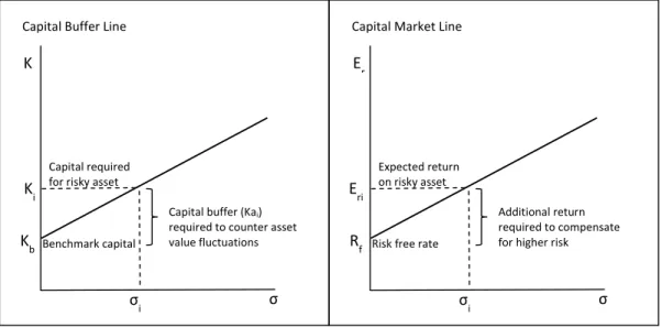
In a stock market context beta (β) measures the systematic risk of an individual security with CAPM predicting what an asset or portfolio’s expected return should be relative to its risk and the market return. As CAPM is a widely used model, we will not explain it in detail, other than a brief summary and an explanation of our modifications. Within CAPM is the Capital Market line (CML), where additional volatility (σ) above a benchmark σ or market σ, needs to be compensated for by additional return above the risk free rate (Rf). This is shown
in Figure 1. For CML, E(Ri) is the expected asset return and E(Rm) is the market return:
6
CABM follows a similar thought process to CAPM, but instead of extra returns compensating for share price volatility above a risk-free rate, we measure additional capital required to compensate for additional volatility in market asset values (measured by the Merton DD model) above a specified benchmark. There are some important differences between CAPM and CABM. It measures capital as opposed to returns, it incorporates the Merton model to measure volatility in market asset values as opposed to share price volatility and it uses a capital benchmark as opposed to a risk free rate. A further feature is that it also a default measurement model, as DD (see sections 2.3 and 3) can be measured from the CBL as Ki / σi.
Figure 1. Comparing CABM’s CBL to CAPM’s CML Capital Buffer Line
σ Kb K i K σ i Benchmark capital
Capital buffer (Kai)
required to counter asset
value fluctuations
Capital required
for risky asset
Capital Market Line
σ Rf E ri E r σ i Risk free rate
Additional return
required to compensate
for higher risk
Expected return
7
β is measured as the market asset volatility of asset i (σi) divided by benchmark volatility (σb),
which is the level of market asset volatility associated with a benchmark capital (Kb). Kb is
the prescribed minimum level of capital for any asset in a portfolio:
ߚ ൌఙఙ
್ (2)
CAPM’s CML is re-defined as the Capital Buffer Line (CBL) as shown in Figure 1, which shows additional capital required for risky loan assets. Capital required (Ki) for asset i:
ܭ ൌ ቀఙఙ
್ܭቁ ൌ ߚܭ (3)
Additional capital required for asset i (Kai) to compensate for risk above the benchmark rate:
ܭܽ ൌ ቀఙఙ
್ܭቁ െ ܭ (4)
2.3 The Merton DD Model
Volatility in our model is based on market asset value volatility as per the Merton (1974) Distance to default (DD) model. As the model is well documented, we only provide a brief summary of its key features to assist the reader. Key components of the model are equity (E), market asset values of the firm (V), debt (F) and fluctuations in market asset values (σV). The
firm defaults when liabilities exceed assets. This equals the payoff of a call option on the firm’s value with strike price F. If, at time T, loans exceed assets, then the option will expire unexercised and the owners default. The call option is in the money where VT - F > 0, and out
the money where VT - F < 0. As V-F is a measure of the firm’s capital, in our model V = F is
the point where the lender has run out of capital. An increase in σV indicates capital erosion,
which needs to be restored, as noted by BOE and IMF (see our introduction). Merton assumes that asset values are log normally distributed, and calculates DD (with µ being the drift in asset values) as:
8 T T F V DD V V 0.5 ) ( ) / ln( 2 (5)
There are different ways in which this “capital” numerator can be defined. Basel III has a risk-weighted capital calculation. Capital in an accounting sense is measured as book value of debts minus liabilities. Moody’s KMV (Crosbie & Bohn, 2003), find that in general firms do not default when asset values reach total liability book values, due to the breathing space given by long term liabilities. Thus KMV use current debt plus half of long term debt as the default point (so do we, when applying equation 5 in this paper). Gapen, Gray, Lim, and Xiao (2004) from the IMF, refer to “Distance to Distress” where the capital numerator is measured as market value of assets minus a specified distress barrier. Crosbie and Bohn (2003), provide the following simplified equation:
) ( ) ( V V F V DD (6)
We simplify this even further:
V
K DD
(7)
where K is the capital held as a percentage of the relevant asset or portfolio. If for example capital is 4% and σV is 2%, then DD is 2 standard deviations away from default. In our model,
it is immaterial which formula is used to measure K, as long as the denominator is σV. This is
because we are interested in the relative capital changes brought about by changes in σV,
rather than absolute capital measures. Our benchmark capital (Kb)is the minimum capital
which a bank is required to maintain, and any increase in the σV denominator requires a
proportionately equal increase in the capital numerator to restore the DD.
To derive σV, we obtain daily equity returns per entity, and calculate the standard deviation of
the logarithm of price relatives. Following the estimation, iteration and convergence procedure outlined by KMV (Crosbie & Bohn, 2003) and Bharath and Shumway (2008), we
9
derive asset value returns, allowing for correlation between returns as described by KMV’s Kealhofer and Bohn (1993). These figures are then applied to the DD calculation (equation 5). We measure µ as the mean of the change in lnV as per Vassalou & Xing (2004).
3.
Applications of CABM
We commence our illustration with a single asset portfolio, using an entity from our dataset, Con-way, a transport company. Con-way was hard hit during the GFC through a combination of factors. This included volatility in energy prices and a meltdown of core industries that the company was reliant on such as housing, construction and automotive industries. Prices and margins came under severe pressure. Profits plunged from $147m in 2007 to $67m in 2008, and then to a huge loss of $111m in 2009. Although a small profit was achieved in 2010, which has been steadily climbing since, profits have never returned to pre-GFC levels.
As at 2005, Con-way had an external credit rating of Baa3, which remained unchanged to end 2012, despite the severity of the problems incurred by the company. Under Basel II and Basel III, a bank is required to hold 8% capital, multiplied by the risk weighted assets (RWA), which for a Baa3 rating is 100% under the standardized model, giving an 8% capital requirement. It should be noted that a bank or regulator can choose to opt out of the external ratings approach and hold 100% RWA against all corporate assets, which the US has chosen to do. To compare the results of our model to Basel, we will assume here that a ratings based approach applies, but we also comment on how this would change if opting out. Moody’s state that their ratings show relative risk, rather than absolute risk, but from a Basel perspective this has important ramifications, because an unchanged rating means no change in the capital required throughout the period.
The right hand side of Table 1 shows the RWA, the β applying to the RWA (βRWA, which we
explain in the following paragraph), and the required capital (K) under Basel. Because the capital remains static throughout the period, βis 1 for each year. It should be noted that, when Basel III is eventually fully phased in, banks will also be required to hold a 2.5% capital conservation buffer, which will improve the overall capital situation of a bank. Nonetheless, this falls well short of our CABM outcomes.
10
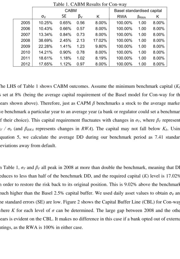
Table 1. CABM Results for Con-way
CABM Basel standardised capital
σV SE βV K RWA βRWA K 2005 10.25% 0.65% 0.56 8.00% 100.00% 1.00 8.00% 2006 10.43% 0.66% 0.57 8.00% 100.00% 1.00 8.00% 2007 13.34% 0.84% 0.73 8.00% 100.00% 1.00 8.00% 2008 38.69% 2.45% 2.13 17.02% 100.00% 1.00 8.00% 2009 22.28% 1.41% 1.23 9.80% 100.00% 1.00 8.00% 2010 14.21% 0.90% 0.78 8.00% 100.00% 1.00 8.00% 2011 18.61% 1.18% 1.02 8.19% 100.00% 1.00 8.00% 2012 17.65% 1.12% 0.97 8.00% 100.00% 1.00 8.00%
The LHS of Table 1 shows CABM outcomes. Assume the minimum benchmark capital (Kb)
is set at 8% (being the average capital requirement of the Basel model for Con-way for the years shown above). Therefore, just as CAPM β benchmarks a stock to the average market, we benchmark a particular year to an average year (a bank or regulator could set a benchmark of their choice). This capital requirement fluctuates with changes in σV, where βV represents
σV / σb (and βRWA represents changes in RWA). The capital may not fall below Kb. Using
equation 5, we calculate the average DD during our benchmark period as 7.41 standard deviations away from default.
In Table 1, σVand βVall peak in 2008 at more than double the benchmark, meaning that DD
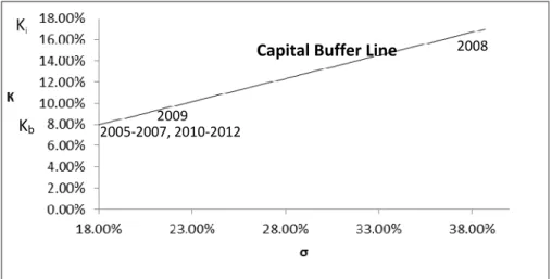
reduces to less than half of the benchmark DD, and the required capital (K) level is 17.02%, in order to restore the risk back to its original position. This is 9.02% above the benchmark, much higher than the Basel 2.5% capital buffer. We used daily asset values to obtain σV and the standard errors (SE) are low. Figure 2 shows the Capital Buffer Line (CBL) for Con-way, where K for each level of σ can be determined. The large gap between 2008 and the other years is evident on the CBL. It makes no difference in this case if a bank opted out of external ratings, as the RWA is 100% in either case.
11
Figure 2: CBL for Con-way
We now extend our analysis from one asset to our portfolio of mid-cap assets. As with our single asset, we base Kb on the average volatility over all the years. The average annual RWA
applying to our portfolio, based on each of the assets’ credit ratings in the portfolio, was 94%. Multiplied by the Basel capital requirement of 8%, this provides a risk weighted capital of 7.5%, which we set as Kb.
Table 2. CABM Results for mid-cap portfolio.
CABM Basel standardised capital
σV SE βV K RWA βRWA K 2003 16.02% 1.01% 0.80 7.50% 95.00% 1.01 7.60% 2004 14.58% 0.92% 0.73 7.50% 91.58% 0.98 7.33% 2005 13.62% 0.86% 0.68 7.50% 91.01% 0.97 7.28% 2006 14.17% 0.90% 0.71 7.50% 91.59% 0.98 7.33% 2007 20.63% 1.30% 1.04 7.77% 81.98% 0.87 6.56% 2008 43.93% 2.78% 2.20 16.53% 88.13% 0.94 7.05% 2009 23.56% 1.49% 1.18 8.87% 95.48% 1.02 7.64% 2010 16.19% 1.02% 0.81 7.50% 100.34% 1.07 8.03% 2011 21.20% 1.34% 1.06 7.98% 102.66% 1.09 8.21% 2012 15.38% 0.97% 0.77 7.50% 101.45% 1.08 8.12% 2005‐2007, 2010‐2012 2009 2008 Kb
12
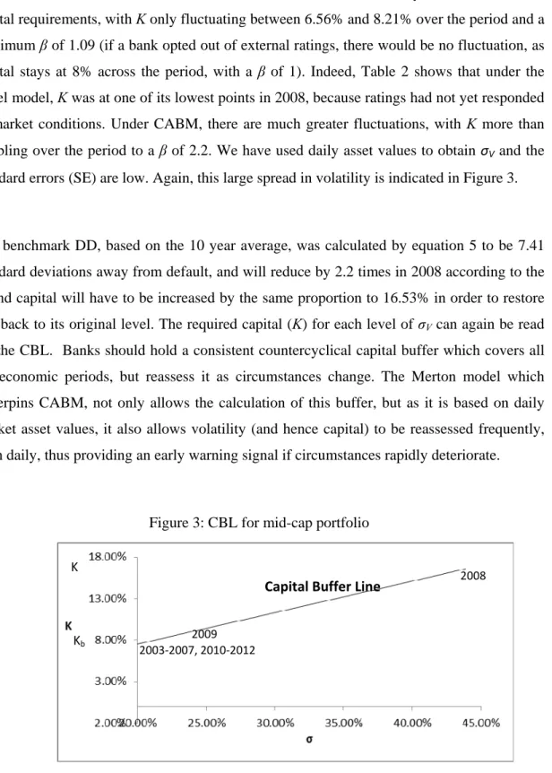
Table 2 shows how under the Basel standardized model, there is very little fluctuation in capital requirements, with K only fluctuating between 6.56% and 8.21% over the period and a maximum βof 1.09 (if a bank opted out of external ratings, there would be no fluctuation, as capital stays at 8% across the period, with a β of 1). Indeed, Table 2 shows that under the Basel model, K was at one of its lowest points in 2008, because ratings had not yet responded to market conditions. Under CABM, there are much greater fluctuations, with K more than doubling over the period to a β of 2.2. We have used daily asset values to obtain σV and the standard errors (SE) are low. Again, this large spread in volatility is indicated in Figure 3.
Our benchmark DD, based on the 10 year average, was calculated by equation 5 to be 7.41 standard deviations away from default, and will reduce by 2.2 times in 2008 according to the
β, and capital will have to be increased by the same proportion to 16.53% in order to restore DD back to its original level. The required capital (K) for each level of σV can again be read
off the CBL. Banks should hold a consistent countercyclical capital buffer which covers all the economic periods, but reassess it as circumstances change. The Merton model which underpins CABM, not only allows the calculation of this buffer, but as it is based on daily market asset values, it also allows volatility (and hence capital) to be reassessed frequently, even daily, thus providing an early warning signal if circumstances rapidly deteriorate.
Figure 3: CBL for mid-cap portfolio
2003‐2007, 2010‐2012
2008
2009
Capital Buffer Line
K
13
In order to be confident in our model, we compare the indicated risk and capital levels to actual default levels experienced for rated entities. We obtain year by year default figures by rating from Moody’s global default database for each of our 10 years, and match these to the rating of every entity in our portfolio. We calculate a weighted average portfolio default β, which in line with our CABM model is based on the maximum annual portfolio default figure divided by the average default figures for ten years. This yields a default β based on Moody’s figures of 2.32, just slightly more than CABM’sβ of 2.20. Given the highly detailed nature of this comparison with actual Moody’s defaults (rating by rating, year by year), this can be considered to be a very extensive and accurate comparison.
As an additional check we compare our results to corporate delinquent loan figures from the U.S. Federal Reserve Bank (2013), which is not as accurate as our comparison to Moody’s default figures as the delinquent loan figures are not split by rating. Nonetheless, it gives an idea of overall corporate default volatility across the market. The β for these delinquent assets, calculated in a similar way to which we calculated our CABM and Moody’s default β, is 1.92, slightly under our CABM Beta of 2.20, but again, much more accurate than the Basel maximum βRWAfor this portfolioof 1.09.
We now turn to policy prescriptions. In addition to the prescribed capital conservation buffer of 2.5%, Basel III requires regulators in each member state to set a countercyclical capital buffers, which are reviewed on a regular basis. CABM could be used at three different policy levels to facilitate these buffer calculations. At the global level, it could be used to modify the Basel standardized model policy, by providing β’s attached to each credit rating. At the member regulator level, β’s could be reviewed on a regular basis as part of the regulator policy for reviewing capital adequacy according to the particular economic circumstances of the member country.
These revised β’s could be provided to Banks with a requirement to adjust buffers. At a bank policy level, banks could use CABM as part of their internal capital adequacy modeling policy. Basel could set the time intervals at which β’s are required to be reviewed by regulators, and regulators could set them for Banks. CABM is extremely flexible in the use of
14
time periods, given that asset values can be measured at any chosen time interval, such as daily, monthly, quarterly, annually, or even longer to cover different cycles.
4.
Conclusions
We have developed an innovative CABM model which is able to measure fluctuations in asset values and the capital that is required to compensate for risk above a benchmark level. The advantages of the model are its simplicity and incorporation of the well-established techniques of CAPM and the Merton DD model. Our comparison to actual defaults show the model to be far more accurate in determining the capital adequacy levels than a ratings based model. During the GFC, the banking industry was beset by capital shortages highlighting the need for improved capital adequacy requirements across dynamic economic circumstances. Given the simplicity and accuracy of the CABM model, it can provide an extremely useful policy tool to Basel, banks and regulators in meeting this need, rather than the current Basel method of applying an across the board capital buffer percentage.
15
References
Bank for International Settlements. (2011). Basel III: A global regulatory framework for more resilient banks and banking systems - revised version June 2011. Retrieved 2 February 2013, from http://www.bis.org
Bank of England. (2008). Financial Stability Report, October. (24).
Bharath, S. T., & Shumway, T. (2008). Forecasting default with the merton distance-to-default model. The Review of Financial Studies, 21(3), 1339-1369.
Bucher, M., Diemo, D., & Hauck, A. (2013). Business cycles, bank credit and crises.
Economics Letters, 120(2), 229-231.
Chan-Lau, J., & Sy, A. (2006). Distance-to-default in banking: A bridge too far: IMF working paper WP06/215.
Crosbie, P., & Bohn, J. (2003). Modelling default risk. Retrieved 12 May 2013, from
http://www.moodysanalytics.com/
European Central Bank. (2005). Financial Stability Review.
Federal Reserve Bank. (2012). The new face of bank capital. Financial Update, 25(3). Federal Reserve Bank. (2013). U.S. Federal Reserve statistical release. Charge-off and
delinquency rates.
Gapen, G., Gray, D., Lim, C., & Xiao. (2004). The contingent claims approach to corporate vulnerability analysis: Estimating default risk and economy-wide risk transfer: International Monetary Fund WP/04/121.
Kealhofer, S., & Bohn, J. R. (1993). Portfolio Management of Default Risk. Retrieved 11 June 2009, from www.moodysanalytics.com
Kretzschmar, G., McNeil, A. J., & Kirchner, A. (2010). Integrated models of capital
adequacy – Why banks are undercapitalised. Journal of Banking and Finance, 34(12), 2838-2850.
Merton, R. (1974). On the pricing of corporate debt: The risk structure of interest rates.
Journal of Finance, 29, 449-470.
Moody's Analytics. (2013). History of KMV. http://www.moodysanalytics.com/About-Us/History/KMV-History.aspx
Sharpe, W. F. (1964). Capital Asset Prices - A theory of market equilibrium under conditions of risk. Journal of Finance, 19(3).
Vassalou, M., & Xing, Y. (2004). Default risk in equity returns. Journal of Finance, 59, 831-868.
Weber, R. F. (2010). New governance, financial regulation, and challenges to legitimacy: The example of the internal models approach to capital adequacy regulation.
Administrative Law Review, 62(3), 783-872.
Woo, S. P. (2012). Stress before consumption: A proposal to reform agency ratings.