A biologically plausible learning rule for deep learning in the brain

A B

IOLOGICALLY

P

LAUSIBLE

L

EARNING

R

ULE FOR

D

EEP

L

EARNING IN THE

B

RAIN

Isabella Pozzi Vision & Cognition Group Netherlands Institute for Neuroscience

Amsterdam, The Netherlands

[email protected]

Sander M. Bohte Machine Learning Group Centrum Wiskunde & Informatica

Amsterdam, The Netherlands

[email protected]

Pieter R. Roelfsema Vision & Cognition Group Netherlands Institute for Neuroscience

Amsterdam, The Netherlands

[email protected]

A

Intelligence is our ability to learn appropriate responses to new stimuli and situations. Recent theoretical insights have allowed a preliminary understanding of how animals learn to represent and memorize the key features of sensory stimuli for the guidance of action, and how this learning can proceed by trial-and-error. However, our understanding of how organisms can learn more complex tasks is still in its infancy. A number of researchers have proposed that deep learning, which is providing important progress in a wide range of high complexity tasks, might inspire new insights into learning processes in the brain. However, the methods used for deep learning in artificial neural networks are biologically unrealistic and would need to be replaced by biologically realistic counterparts. Previously, some biologically plausible learning rules were devised [Roelfsema and Ooyen (2005); Rombouts et al. (2012)], showing promising results. However, these previous studies focused on shallow networks with three layers, and only mentioned the possibility of generalizing the biologically plausible learning schemes to deeper networks with an arbitrary number of layers. Will these learning rules also generalize to networks with more layers and can they handle tasks of higher complexity? Here, we demonstrate that these learning schemes indeed generalize to networks with an arbitrary number of layers if we include an attention network that propagates information about the selected action to lower network levels. The resulting learning rule is equivalent to a particular form of error-backpropagation that trains one output unit at anyone time. To demonstrate the utility of the learning scheme in larger problems we include simulations with a network with two -hidden-layers that is trained on the MNIST dataset, i.e. a standard and interesting Machine Learning task. Our results demonstrate that the capability of the new biologically plausible learning rule (called Q-AGREL) is comparable to error backpropagation. However, its learning rate is 1.5-2 times slower because the network trains one output unit at a time in a reinforcement learning setting and it therefore has to discover the appropriate outputs by trial-and-error, unlike supervised backpropagation where the correct response is signaled by an external teacher and the connections to all output units are updated at the same time. Our results provide new insights into how deep learning can be implemented in the brain.

Keywords Reinforcement learning·MNIST·deep learning·biologically plausible learning rules

1

Introduction

Imagine a human or monkey in front of a screen, who has to decide which action gives the reward, e.g. money or fruit juice. The subject does not yet know the rules behind the task, and he does not know when the task finishes or when the rules change. Yet through trial-and-error, humans and animals can learn complicated tasks, even if the only feedback is the presence or absence of reward at the end of each trial. Understanding this learning process of mapping new stimuli and new situations onto appropriate actions, is a central question in both AI and Neuroscience.

There are various types of learning rules for neural networks. In unsupervised learning, the network learns the statistical regularities of the sensory input without any feedback about desired performance. In supervised learning a teacher provides the desired pattern of activity of the output layer of the network, for every stimulus. A weak form of supervision is reinforcement learning where the network or agent explores its environment and receives rewards or punishments for selected actions, but the most rewarding actions have to be discovered by the agent because there is no teacher. As a result, learning is slower in reinforcement learning than in the case of fully supervised learning. An important virtue of reinforcement learning is that it also occurs in animals and humans. Hence, reinforcement learning by artificial neural networks can be used as a model for learning in the brain [Bishop et al. (1995)]. Indeed, previous theories have suggested how powerful reinforcement learning rules inspired by artificial neural networks could be implemented in the brain [Roelfsema and Holtmaat (2018)] and the methodology for shaping neural networks with rewards and punishments is an active area of research [Schmidhuber et al. (2011); Friedrich et al. (2010); Vasilaki et al. (2009); O’Reilly and Frank (2006); Huang et al. (2013)].

Artificial neural networks with many layers are calleddeep[Hinton et al. (2006)] and they have recently accomplished breakthrough performance on important tasks, like image and speech recognition [Krizhevsky et al. (2012); Hinton et al. (2012)]. Deep artificial neural networks are typically trained with supervised learning methods and in particular with the error-backpropagation rule, a method that specifies how connections between the units of a network should change during training. The error backpropagation adjusts synaptic weights in networks that are composed of several layers to reduce the errors in the mapping of inputs into the lower layer to outputs in the top layer. It does so by first computing the output error, which is the difference between the actual and desired activity levels of output units. Error backpropagation then determines how the strength of connections between successively lower layers should change to decrease this error, by computing derivatives using gradient descent [Rumelhart et al. (1986)]. Artificial neural networks, trained by error backpropagation, now attain human-level performance in image recognition [LeCun et al. (2015)] and in some (computer) games [Mnih et al. (2015); Silver et al. (2017)].

The brain of humans and animals are also composed of many layers between the sensory neurons that register the stimulus and the motor neurons that control the muscles. Hence it is tempting to speculate that the methods for deep learning that work so well for artificial neural networks also play a role in the brain Marblestone et al. (2016); Scholte et al. (2017). A number of important challenges need to be solved, however, and some of them were elegantly expressed by Francis Crick who argued that the error-backpropagation rule is neurobiologically unrealistic [Crick (1989)]. He found it difficult to imagine how synapses in the brain could determine the change in their strength that would decrease the overall network error; that is, how can they compute the error derivative based on information available locally, at the synapse? In more recent years, researchers have started to address this challenge by proposing ways in which learning rules that are equivalent to error-backpropagation might be implemented in the brain [Urbanczik and Senn (2014), Schiess et al. (2016); Scellier and Bengio (2017); Roelfsema and Ooyen (2005); Rombouts et al. (2015); Brosch et al. (2015)], which were reviewed in [Marblestone et al. (2016)].

One of the main challenges remained to inform synapses at the lower network levels about the desired change in their strength, because the influence of changes in their strength on activity in the output layer is only indirect and depends on many intermediate synapses. Here we will focus on a particular type of learning rule known as AGREL (attention-gated reinforcement learning) [Roelfsema and Ooyen (2005)] and AuGMEnT (attention-gated memory tagging) [Rombouts et al. (2015)]. These learning rules realized that in a reinforcement learning setting the synaptic error derivative can be split into two factors. The first factor is the reward prediction error (RPE) during reinforcement learning. The RPE is positive if an action selected by the network is associated with more reward than expected or if the prospects of receiving reward increase and the RPE is negative if the outcome of the selected action is disappointing. In the brain, the RPE is signaled by neuromodulatory systems that project diffusely to many synapses so that they can inform them about the RPE [Schultz (2002)]. The second factor is an attentional feedback signal that is known to propagate from the motor cortex to earlier processing levels in the brain [Roelfsema and Holtmaat (2018); Pooresmaeili et al. (2014)]. When a network chooses an action, this feedback signal is most pronounced for those neurons and synapses that can be held responsible for the selection of this action and hence for the resulting RPE. These two factors jointly determine synaptic plasticity. Importantly, the learning rules cause the strength of feedback connections to become proportional to that of the feedforward connections, and the learning rules then become computationally equivalent to error backpropagation on the error in the value of the selected action. A recent study in humans demonstrated the separable influences of

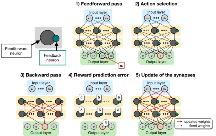
1) Feedforward pass 2) Action selection Output layer 0.1 0.5 0.2 Input layer xN x1 0.1 qs Output layer 0 1 0 Input layer xN x1 0 Feedforward neuron _Feedback neuron

3) Backward pass 4) Reward prediction error

Output layer 0 1 0 Input layer xN x1 0 Output layer 0 1 0 Input layer xN x1 0 ẟ ẟ ẟ ẟ ẟ ẟ ẟ

5) Update of the synapses

Output layer 0 0 Input layer xN x1 0 1 updated weights fixed weights

Figure 1:Schematic depiction of Q-AGREL. At each node, a feedforward neuron (grey) and a feedback neuron (green) are present; two sets of weights, i.e. feedforward and feedback weights, connect the nodes in the network. 1) In the feedforward pass, the information is inferred from the input layer throughout the network, until the ouput layer, where the Q-values are computed; 2) based on the Q-values, an action is selected as described in the text; 3) the activity of the winning unit is propagated back through the feedback connections to the feedback neurons; 4) a reward prediction errorδis globally computed; 5) the synapses (both feedforward and feedback, even if the latter are not indicated in the image) are updated.

rewards and attention on the learning of new stimulus-response associations [Vartak et al. (2017)]. Furthermore, as both factors are available at the synapses undergoing plasticity, it has been argued that learning schemes such as AGREL and AuGMEnT are indeed implemented in the brain [Roelfsema and Holtmaat (2018)].

The previous AGREL and AuGMEnT models used networks with only three layers, that is, a single hidden layer, and modeled learning in tasks with only a handful input neurons. The present work has two goals. The first is to establish the relation between the biologically realistic learning rules and error backpropagation for deep networks composed of multiple layers between the input and output layer in a reinforcement learning setting. Can the brain, with its many layers between input and output indeed solve the credit-assignment problem in a manner that is equivalent to deep learning? The second goal is to compare trial-and-error learning with biologically plausible learning rules to learning with error-backpropagation in more challenging problems. To this aim we investigated if and how the biologically learning rules cope with the MNIST data for handwritten digit recognition. We will present a binary image to the network, it chooses a digit category and immediate feedback is given about whether the choice is right or wrong.

2

Deep, biologically plausible reinforcement learning

We here generalize and extend AGREL to networks with multiple layers with two modifications of the previous learning schemes. Firstly, we use rectified linear (ReLU) functions as activation function of the neurons in the network. This simplifies the learning rule, because the derivative of the ReLU is equal to zero for negative activation values, and has a constant positive value for positive activation values. We note, however, that the learning scheme could be generalized to other activation functions. Secondly, we assume that network nodes correspond to cortical columns with feedforward and feedback subnetworks: in the present implementation we use a feedforward neuron and a feedback neuron per node, shown as grey and green circles inFig. 1.

Overall, the network learning goes through five phases upon presentation of an input image (Fig. 1): (1) the signal is propagated through the network by feedforward connections to obtain activations for the output units that estimate the value of each of the choices (Feedforward pass), (2) in the output layer one output unit is chosen (Action selection), (3) the selected output unit causes (attention-like) feedback to the feedback unit of each node (Backward pass). Note that this feedback network propagates information about the selected action (just as in the brain see e.g. [Roelfsema and Holtmaat (2018)]), and that it does not need to propagate error signals, which would be biologically implausible. (4) A reward prediction errorδis computed and signaled throughout the network, and (5) the strengths of the synapses are updated.

The proposed learning rule, Q-AGREL, has four factors:

∆wi,j=prei·postj·δ·f bj, (1)

where∆wi,jis the change in the strength of the synapse between unitsiandj,preiis a function of the activity of the presynaptic unit,postja function of the activity of the postsynaptic unit andf bjthe amount of feedback from the selected action arriving at feedback unitjthrough the feedback network. This local learning rule governs the plasticity of both feedforward and feedback connections between the nodes.

To understand the learning rule, it is important to describe the interactions between the feedforward and feedback units within a node. The role of the feedback units in the node is to gate the plasticity of feedforward connections (as well as their own plasticity). In Equation 1,f bjacts as a plasticity-gating term, which determines the plasticity of synapses onto the feedforward neuron. There is neuroscientific evidence for the gating of plasticity of feedforward connections by the activity of feedback connections, as was reviewed by [Roelfsema and Holtmaat (2018)].

In the opposite direction, the feedforward units gate the activity of the feedback units. Feedback gating is shaped by the local derivative of the activation function, which, for a unit with a ReLU activation function, corresponds to an all-or-nothing gating signal: for ReLU feedforward units, the associated feedback units of a node are only active if the feedforward units are activated above their threshold. Otherwise the feedback units remain silent and they do not propagate the feedback signal to lower processing levels.

Gating of the activity of feedback units by the activity of feedforward units is in accordance with neurobiological findings: attentional feedback effects on the firing rate of sensory neurons are pronounced if the neurons are well driven by a stimulus and much weaker if they are not [Van Kerkoerle et al. (2017); Roelfsema (2006); Treue and Trujillo (1999)].

In what follows we will first consider learning by a network with two fully connected hidden layers comprised of ReLU units (Fig. 1), and we will then explain why the proposed learning scheme can train networks with an arbitrary number of layers in a manner that provides synaptic changes that are equivalent to a particular form of error backpropagation. In the network with two hidden layers, there areNinput units with activitiesxi. The activation of theJneurons in the first hidden layer,y_j(1), is given by:

y(1)_j =ReLUa(1)_j with a(1)_j =

N X

i=1

ui,jxi, (2)

whereui,jis the synaptic weight between thei-th input neuron and thej-th neuron in the first hidden layer, and the ReLU function can be expressed as:

ReLU(x) =

_x

if x >0,

0 otherwise. (3)

Similarly, the activations of theKneurons in the second hidden layer,y(2)_k , are obtained as follows:

y_k(2)=ReLUa(2)_k with a(2)_k = J X j=1 vj,ky (1) j , (4)

withvj,kas synaptic weight between thej-th neuron in the first hidden layer and thek-th neuron in the second hidden layer. TheLneurons in the output layer are fully connected (by the synaptic weightswk,l) to the second hidden layer and will compute a linearly weighted sum of their inputs:

ql= K X k=1 wk,ly (2) k , (5)

which we treat as Q-values as defined in Reinforcement Learning [Sutton et al. (1998)], from which actions (or classifications) are selected by an action selection mechanism.

x

fb

x

fb

y

y

y

y

ẟ

ẟ

ẟ

ẟ

ẟ

ẟ

u

_1,

′

N

v

u

_N

_,1

v

′

y

₁

(1)

a

fb

_y

(1)

1

fb

_y

g

(1)

x

g

fb

Δ

u

=

αδx

g

fb

≡

Δ

u

′

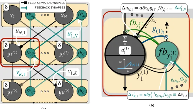
Figure 2:Details of the Q-AGREL algorithm. (a)Explanatory sketch of the notation used. The feedforward (grey) and feedback (green) weights are indicated, together with the activation of the neurons (e.g.y₁(1)for the feedforward neuron andf b_y(1)

1

for the respective feedback neuron);(b)details on a single-neuron level. During the forward pass, the feedforward neuron receives a set of weighted inputs, which are summed, obtaining the net input to the neuron (i.e. a(1)₁ ), which will be passed to a ReLU function. During the backward pass, the feedback neuron activation (f b_y(1)

1 ) is gated by the factorg(1)1(i.e. plasticity gating). During the weight update,y

(1)

1 andf by(1)₁ are used to update the synapses at the feedback and feedforward neuron, respectively (synapse gating). It can be seen how all the information is locally available for the update, both for the feedback and feedforward synapses.

In our action selection mechanism, the output unit with the highest activity has the largest chance of being selected. After action selection, the activity of the winning unit is set to one and the activity of the other units to zero. For the action-selection process, we implemented a max-Boltzmann controller [Wiering and Schmidhuber (1997)]: the network will select the output unit with the highest Q-value as the winning unit with probability1−, and otherwise it will probabilistically select an output unit using a Boltzmann distribution over the output activations:

P(zl= 1) =

expql P

lexpql

. (6)

Once an action is selected, the network will receive a scalar rewardrand a globally available RPEδis computed as:

δ=r−qs, (7)

whereqsis the activity of the winning units(seeFig. 1), i.e. zl=s= 1andzl6=s= 0, leading to a global prediction errorE=1₂δ2. In a classification task, we set the reward to 1 when the selected output unit corresponds to the correct class, and we set the reward to 0 otherwise.

Next, only the winning output unit starts propagating the feedback signal – the other output units are silent. This feedback will pass through the feedback connections with their own weightsw0to the feedback neurons in the next layer, where the feedback signal is gated by the local derivative of the activation function, and then further passed to the next layer of feedback neurons through weightsv0, and so on. We will demonstrate that this feedback scheme locally updates the synapses of the network in a manner equivalent to a particular form of error-backpropagation.

Given the learning rateα, the update of the feedforward weightswk,sbetween the last hidden layer and the output layer (but the same rule holds for the corresponding set of feedback weights, indicated asw_s,k0 ) is given by:

∆wk,s=αδy

(2)

x

x

y

y

y

y

if

g

= 1

g

x

x

y

y

y

y

if

g

= 0

g

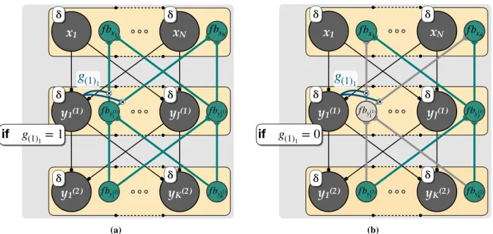
Figure 3:Effects of the plasticity-gating mechanisms on the feedback signal.(a)Open gate. Because the activation of the neurony₁(1)is positive, the gate is open and the feedback signalf b_y(1)

1

is received by the feedback neurons in the next layer (i.e.f bx1, . . . , f bxN);(b)Closed gate. The gate switches off when the input to the feedforward unity

(1)

1 stay

below the threshold for activation and now the plasticity gating feedback signal is not propagated to the next lower layer (i.e. the grey elements in the figure).

Note that the synaptic changes only depend onδ, the RPE and pre- and post-synpatic activity. The feedforward and feedback weightsvandv0between the first and second hidden layer change as follows:

∆vj,k=αδy (1) j g(2)kws,kzs=αδy (1) j g(2)kf by_k(2) = ∆v 0 k,j, with g(2)k = ( 1 if y_k(2)>0, 0 otherwise, (9) f b_y(2) k =X l g(O)lw 0 l,kzl=ws,k0 zs, (10) which is the feedback coming from the output layer. Hence, the synaptic plasticity rule depends on the RPE, the pre-and postsynaptic activity pre-and the activity of the feedback neuronf b_y(2)

k

. Finally, the weightsubetween the inputs and the first hidden layer are adapted as:

∆ui,j=αδxig(1)j X k v0k,jg(2)kw 0 s,kzs =αδxig(1)j X k v0_k,jg(2)kf by_k(2)=αδxig(1)jf by(1)_j , with g(1)j = ( 1 if y_j(1)>0, 0 otherwise, (11) f b_y(1) j =X k g(2)kv 0 kjf by(2)_k , (12)

which is the feedback coming from the second hidden layer. Again, the plasticity depends on pre- and postsynpatic activity, the RPE and the activity of the feedback unitf b_y(1)

j

in the column.f b_y(2)

k

andf b_y(1)

j

represent the activity of feedback neuronsy_k(2)andy_j(2), which are activated by the propagation of signals through the feedback network once an action has been selected (see alsoFig. 2).

In general, for even deeper networks, updates of feedforward synapses∆wp,mfromp-th neuron in then-th hidden layer ontom-th feedforward neuron in the(n+ 1)-th hidden layer are thus computed as:

∆wp,m =αδy(pn)g(n+1)_mf b_y(n+1)

and it is equal to the update of the corresponding feedback synapse∆wm,p0 , where the activity of the feedback unit is determined by the feedback signals coming from the(n+ 2)-th hidden layer as follows:

f b_y(n+1) m = X q g(n+2)_qv0q,mf b_y(n+2) q , (14)

withqindexing the units of the(n+ 2)-th hidden layer.

The update of a synapse is thus expressed as the product of four factors: the RPEδ, the activity of the presynaptic unit, the activity of postsynaptic feedforward unit and the activity of feedback unit of the same postsynaptic node, as anticipated in Equation 1. Notably, all the information necessary for the synaptic update is available locally, at the synapse. Moreover, the identical update for both feedforward and corresponding feedback synapses (i.e.,∆wk,land

∆w0_l,k,∆vj,kand∆vk,j0 , and∆ui,jand∆u0j,i) can be computed locally (see alsoFig. 2b).

For clarity, we reiterate the two main features of the proposed learning rule, which can also be considered as predictions for neurobiological experiments. First, the feedback units gate the plasticity of feedforward connections into the same node (Fig. 2b). The plausibility of this prediction has been discussed by [Roelfsema and Holtmaat (2018)]. Second, if the feedforward unit of a particular node (or cortical column) is not active (its input remains below the ReLU threshold), the associated feedback units are switched off (Fig. 3b). This switching off of feedback units has consequences for the propagation of the feedback signals to lower network levels and hence for the plasticity at these levels, as is illustrated inFig. 3.

We next demonstrate that Q-AGREL is equivalent to a special form of error-backpropagation. In this form the network only computes the derivatives relative to the error of the Q-value of the selected output unit.

For supervised error backpropagation in the same networks with errorEcomputed as the summed square error over all output Q-valuesqland target outputsqˆl,E = 1₂P_l(ql−qˆl)2, if we define ∂E_∂q

l = (ql−qˆl) :=e

(O)

l , where the superscript(O)stands for output layer, the relevant equations for the synaptic updates are:

∆wk,l=−αy (2) k e (O) l , (15) ∆vj,k=−αy (1) j y (2) k 0X l wl,ke (O) l =−αy (1) j y (2) k 0 e(2)_k , (16) ∆ui,j =−αxiy (1) j 0X k vk,jy (2) k 0X l wl,ke (O) l =−αxiy (1) j 0X k vk,jy (2) k 0 e(2)_k =−αxiy (1) j 0 e(1)_j , (17)

and in general, for a weight between unitspandmin layernandn+ 1respectively:

∆wp,m=−αy(pn)y (n+1) m 0 e(_mn+1), with e(_mn+1)=: ∂E ∂y(mn+1) =X q wm,qy(qn+2) 0 e(_qn+2), (18)

withqindexing the units of the(n+ 2)-th hidden layer and<·>0indicating the derivative.

This corresponds to the Q-AGREL equations for the adjustment to the winning output when we sety()_j0 =gj and e(_l=O_s)=_∂q∂E s =−δ, ande (O) l6=s= 0: ∆wk,l=αδy (2) k , (19) ∆vj,k=αδy (1) j gkf b_y(2) k , (20) ∆ui,j =αδxigj X k gkwl,kf b_y(2) k =αδxigjf b_y(1) j , (21) and, by recursion, ∆wp,m=αδyp(n)gmf b_y(n+1) m . (22)

Compared to supervised error-backpropagation, in the RL formulation of Q-AGREL only the errorelfor the winning actionlis non-zero, and the weights in the network are adjusted to reduce the error for this action only. Depending on the selection mechanism that determines winning actions from Q-values, this trial-and-error approach will adjust

the network towards selecting the correct action, while the Q-values for incorrect actions will be trained to just be sufficiently smaller than the correct action so that they are unlikely to be selected. These Q-values will only further decrease in strength occasionally, when the stochastic action takes an explorative action. This in contrast to standard error-backpropagation, which will continuously drive the values of the incorrect actions to the appropriate lower action values. Furthermore, reinforcement learning of Q-values by Q-AGREL is expected to be slower than learning with fully supervised error-backpropagation where a teacher provides the correct Q-values for all actions. We will test these predictions in our simulations.

3

Experiments

We tested the performance of Q-AGREL for fully connected neural networks with one and two hidden layers on the MNIST dataset. MNIST is a classification task, and it is therefore simpler than the more general reinforcement learning settings that necessitate the learning of a number of intermediate actions before a reward can be obtained, and for which AuGMEnT was developed. Like AuGMEnT, Q-AGREL computes reward expectancy in the form of Q-values and it selects actions with an action-selection mechanism. We chose this approach because it gives rise to more stable learning as compared to AGREL, which uses separate action and critic networks.

The MNIST dataset consists of 60,000 training samples, of which 1,000 were randomly chosen for validation at every epoch, and of 10,000 test samples. Every sample is an image of 28 by 28 pixels, and the samples were presented in batches to the network (i.e.batch gradient) to speed up the learning process (but the learning scheme also works with learning after each trial, i.e. not in batches): 100 samples were given as an input, the gradients were calculated, divided by the batch size, and then the weights were updated, for each batch until the whole training dataset was processed (i.e. for 590 batches in total), indicating the end of anepoch. Once every five epochs, a validation accuracy was calculated on the validation dataset. An early stopping criterion was implemented: if for five consecutive times the validation accuracy was the same with one decimal precision, learning was stopped. Otherwise, we trained the networks for 1,000 epochs in total, and at the 500-th epoch the learning rate was decreased to facilitate the convergence. By randomly choosing the validation set in every epoch, the convergence criterion was met more quickly, because the networks train effectively on the whole training dataset, so also on the validation set, throughout different epochs.

We ran the same experiments with Q-AGREL and with error backpropagation with 10 different seeds for synaptic weight initialization. All weights were randomly initialized within the range [−0.05,0.05]and layers were fully connected. We demonstrated in the above that the changes of synaptic weights of Q-AGREL are identical to those of error-backpropagation for one of the output units at a time, provided that the strengths of the feedforward connections between nodes are proportional to the strength of the feedback connections. This reciprocity could emerge as the result of the learning rules described above (see also [Roelfsema and Ooyen (2005)]).

Here we therefore compared the performance of networks where (1) the feedback synapses were identical to the feedforward synapses (strict reciprocity), (2) with independently randomly initialized feedback weights (random

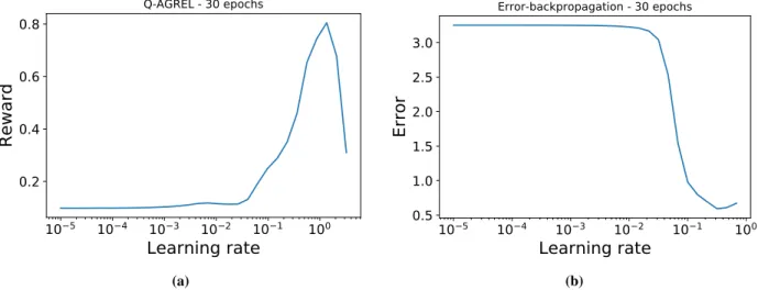
10−5 ₁₀−4 ₁₀−3 ₁₀−2 ₁₀−1 ₁₀0 Learning rate 0.2 0.4 0.6 0.8 R ew ar d Q-AGREL - 30 epochs (a) 10−5 ₁₀−4 ₁₀−3 ₁₀−2 ₁₀−1 ₁₀0 Learning rate 0.5 1.0 1.5 2.0 2.5 3.0 Er ro r Error-backpropagation - 30 epochs (b)

Figure 4:Learning rate optimization study. (a)Curve followed by the Reward throughout the Q-AGREL learning process, as a function of the increasing learning rate;(b)trend of the Epoch error when the learning rate is increased during error backpropagation.

feedback learning) which are expected to become approximately reciprocal during the learning process and (3) networks with so-calledfeedback alignment[Lillicrap et al. (2016)], for which the feedback synapses were randomly initialized but not updated during learning. We note that the networks with feedback alignment thereby violated one of the conditions required for the equivalence between Q-AGREL and error-backpropagation.

We optimized the learning rateαfor each learning rule. Following a similar procedure as the one described in [Smith (2017)], we selected an interval of values for the learning rate for each rule. Then a small simulation (i.e. 30 epochs) was performed, during which the learning rate was increased at each epoch. At the end, the error (in the case of error-backpropagation) or the reward (for Q-AGREL) was plotted as a function of the learning rate, and a value ofα lying within the range with the steepest decrease in error (for backpropagation) or increase in reward (for Q-AGREL) was chosen for the simulations (Fig. 4). The steepest increase in the reward for Q-AGREL was for anαbetween 0.5 and 1, and the steepest decrease in the error for error-backpropagation was for anαbetween 0.05 and 0.1.

4

Results

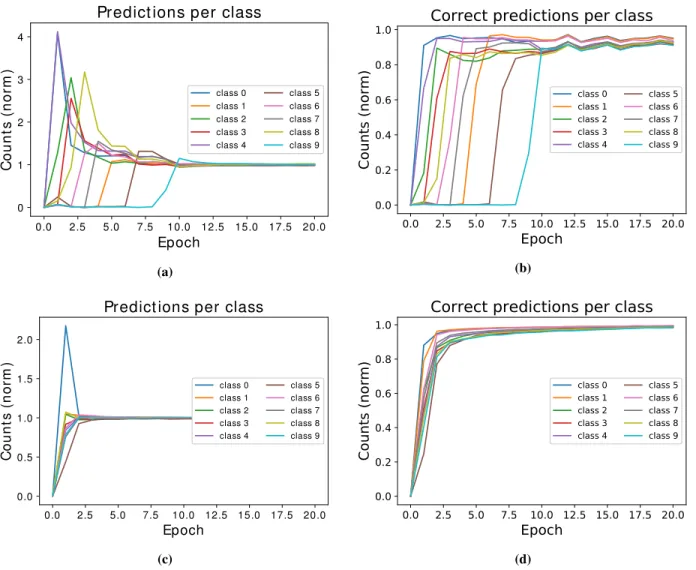
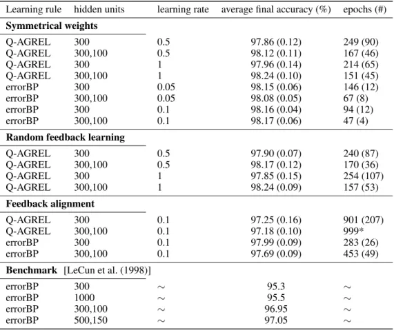
To illustrate the learning process of networks trained with the Q-AGREL reinforcement learning approach, we show how the reward probability increases (Fig. 5a) during the training for one example network. Both the reward obtained at each batch and at each epoch (i.e. average reward over 59 batches, since for this example a batch size of 1,000 was used) are plotted. The panel on the right of theFig. 5illustrates the improvement in performance of one example network that was trained with standard error-backpropagation. An unexpected observation was that learning proceeded in a stepwise manner for Q-AGREL, which contrasts with the smoother progression with standard error-backpropagation. When we analyzed this result, we found that the network discovered each of the 10 digit classes at a time. When it happened to select a new class during the presentation of a digit of the same class (i.e. a coincidental correct response) as the result of the random action selection policy, it quickly started to recognize most samples of the same class.

To substantiate this interpretation, we computed the confusion matrix as function of learning time for an example network trained with Q-AGREL. We evaluated the frequency with which the different classes were selected by the network (Fig. 6a) and we also determined the probability of a correct response for each of the classes (Fig. 6b). It can be seen that from the moment onwards where a new class is recognized, e.g. class "1" at the∼4-th epoch or class "5" at the∼6-th epoch, the network quickly learns how classify multiple images falling within this class. The network exhibits a tendency to then also apply this class label to images that do not belong to the class (note the initial overshoot in the count inFig. 6a) that disappears with more learning. For a comparison, inFig. 6candFig. 6dthe results for error-backpropagation are shown. Here, the network starts recognizing all the classes from the first moment because the teacher always provides the correct response. This leads to faster learning with error-backpropagation than with Q-AGREL. Moreover, in Q-AGREL only the synapses that have impact on the selected are changed, whereas error-backpropagation also decreases the activity of the connections leading to the output units that should remain off. It is therefore evident that training with Q-AGREL should overall take more time than training with error backpropagation.

0 5 10 15 20 Epoch 0.0 0.2 0.4 0.6 0.8 1.0 R ew ar d Q-AGREL Epoch reward Batch reward (a) 5 10 15 20 Epoch −1.0 −0.5 0.0 0.5 1.0 1 - Er ro r Error-backpropagation (b)

Figure 5: Example of learning process (the first 20 epochs are shown) with the two learning schemes in example networks. In both cases two hidden layers were used, the batch size was 1,000 and the learning rate wasα= 0.5.(a) Reward during a Q-AGREL simulation. A step-like trend is observable;(b)evolution of the error (here plotted as 1-error) during an error-backpropagation experiment.

Table 1presents the results of simulations with the different learning rules. In our first simulation, we compared error-backpropagation to a version of Q-AGREL in which the feedback and the feedforward weights were symmetrical. We trained networks with only one hidden layer (with 300 units) and networks two hidden layers; these networks had an extra hidden layer with 100 units. We compared the results obtained with two learning rates and we used 10 seeds for each combination of learning rate and network architecture and report the results asmean (standard deviation)

(Table 1).

Our first result is that Q-AGREL reaches a relatively high classification accuracy of 97.9-98.2% on the MNIST task, obtaining essentially the same performance as standard error-backpropagation. The convergence rate of Q-AGREL was a factor of 2 to 3 slower than that of error-backpropagation. However, this consideration should not distract from the conclusion that Q-AGREL is able to learn the MNIST classification task with a performance that is on par with standard error-backpropagation.

It is also of interest that the addition of an extra hidden layer improved performance, both for networks trained with error-backpropagation and Q-AGREL, albeit only slightly. This difference in final accuracy between the one-hidden-layer networks and their two-hidden-layers counterparts is not as large as was reported originally by [LeCun et al. (1998)] (bottom of theTable 1), and we obtain significantly higher accuracies both for Q-AGREL and error-backpropagation

0.0 2.5 5.0 7.5 10.0 12.5 15.0 17.5 20.0 Epoch 0 1 2 3 4 C ou n ts ( n or m )

Predictions per class

class 0 class 1 class 2 class 3 class 4 class 5 class 6 class 7 class 8 class 9 (a)

0.0 2.5 5.0 7.5 10.0 12.5 15.0 17.5 20.0

Epoch

0.0

0.2

0.4

0.6

0.8

1.0

Co

un

ts

(no

rm

)

Correct predictions per class

class 0 class 1 class 2 class 3 class 4 class 5 class 6 class 7 class 8 class 9 (b) 0.0 2.5 5.0 7.5 10.0 12.5 15.0 17.5 20.0 Epoch 0.0 0.5 1.0 1.5 2.0 C ou n ts ( n or m )

Predictions per class

class 0 class 1 class 2 class 3 class 4 class 5 class 6 class 7 class 8 class 9 (c)

0.0 2.5 5.0 7.5 10.0 12.5 15.0 17.5 20.0

Epoch

0.0

0.2

0.4

0.6

0.8

1.0

Co

un

ts

(no

rm

)

Correct predictions per class

class 0 class 1 class 2 class 3 class 4 class 5 class 6 class 7 class 8 class 9 (d)

Figure 6: Selection frequency for each of the classes for a network trained with Q-AGREL and one with error-backpropagation (the same networks asFig. 5a andFig. 5b, respectively). (a) Frequency of class selection over the epochs for Q-AGREL;(b)Correct predictions per class over the epochs for Q-AGREL. It is possible to notice a correspondence between when the network "discovers" a new class and a step in the learning in Fig. 5a; (c) Frequency of selection across epochs for error-backpropagation;(d)Correct predictions per class over the epochs for error-backpropagation: the network quickly learns to select all the classes.

Table 1:Results (averaged over 10 different seeds, the mean and standard deviation are indicated). In some cases, the network did not converge at the end of the simulation (i.e. after 1000 epochs), even if the learning rate was 10 times smaller from the 500-th epoch.

Learning rule hidden units learning rate average final accuracy (%) epochs (#) Symmetrical weights Q-AGREL 300 0.5 97.86 (0.12) 249 (90) Q-AGREL 300,100 0.5 98.12 (0.11) 167 (46) Q-AGREL 300 1 97.96 (0.14) 214 (65) Q-AGREL 300,100 1 98.24 (0.10) 151 (45) errorBP 300 0.05 98.15 (0.06) 146 (12) errorBP 300,100 0.05 98.08 (0.05) 67 (8) errorBP 300 0.1 98.16 (0.04) 94 (12) errorBP 300,100 0.1 98.17 (0.06) 47 (4)

Random feedback learning

Q-AGREL 300 0.5 97.90 (0.07) 240 (87) Q-AGREL 300,100 0.5 98.17 (0.12) 170 (36) Q-AGREL 300 1 97.85 (0.15) 254 (107) Q-AGREL 300,100 1 98.24 (0.09) 157 (53) Feedback alignment Q-AGREL 300 0.1 97.25 (0.16) 901 (207) Q-AGREL 300,100 0.1 97.18 (0.10) 999* errorBP 300 0.1 97.99 (0.09) 283 (26) errorBP 300,100 0.1 97.69 (0.09) 453 (49)

Benchmark [LeCun et al. (1998)]

errorBP 300 ∼ 95.3 ∼

errorBP 1000 ∼ 95.5 ∼

errorBP 300,100 ∼ 96.95 ∼

errorBP 500,150 ∼ 97.05 ∼

than this original study. Likely causes for these differences are the use of sigmoidal activation functions by [LeCun et al. (1998)] whereas we included ReLU’s, and the smaller number of training epochs in the original study.

As was mentioned in the above, Q-AGREL is equivalent to a form of error-backpropagation in which the Q-value of one output unit is updated per trial, but only if the strengths of feedforward and feedback connections are proportional. However, such proportionality may not be present at the start of the training process in biology and may need to emerge during learning. In the second section of the table, we therefore also report results from networks trained with Q-AGREL with independently initialized feedback weights. The final accuracies and learning rate were indistinguishable from those obtained with Q-AGREL in the case of symmetric weights, which supports our conjecture that the approximate symmetry of feedforward and feedback connections can emerge during learning.

A number of recent studies [Lillicrap et al. (2016)] have demonstrated that forms of learning in networks with one or more hidden layers can also occur when the feedback weights are random and not changed during learning. These previous studies demonstrated that the feedforward connections tend to align in strength with the feedback connections, which is why this process has been called "feedback alignment". In our simulations, we also included networks which were trained with such fixed feedback weights. However, these networks achieved substantially lower accuracies and required many more epochs. Furthermore, we had to lower the learning rate compared to that used with networks trained with Q-AGREL to obtain reasonable results in this feedback alignment framework.

5

Discussion

We here implemented a deep, biologically plausible reinforcement learning scheme called Q-AGREL and found that it was able to train networks with one or two hidden layers to perform the MNIST task with performance that was nearly identical to error-backpropagation. We also found that the trial-and-error nature of learning to classify with

reinforcement learning incurred a very limited cost of 2-3x more training epochs to achieve the stopping criterion. We observed that the learning progressed in a step-wise manner, because the network discovered the usage of the different classes one by one. This result suggests that small modifications might speed up the learning with Q-AGREL. First, it is possible to initialize the Q-values of all actions at higher values, which should increase the network’s tendency to sample all actions from the start. Second, the action selection mechanism could be modified to increase the probability of selecting actions that have not been sampled for a while. Future studies could examine if these and related modifications further speed up the learning process.

The results were obtained with relatively simple network architectures (fully connected layers) and learning rules (no optimizers or data augmentation methods were used). These additions would almost certainly further increase the final accuracy of the Q-AGREL learning scheme. For example, by simply adding distortions algorithms [Cire¸san et al. (2012))] obtained an accuracy on MNIST of 99.68% using networks with only fully connected layers, which is comparable to state-of-the-art convolutional neural networks. Interestingly, Cire¸san et al. found that adding hidden layers had only limited effect on the accuracy that could be achieved, and they obtained an accuracy of 98.22% and 98.15% for one-hidden-layer and two-hidden-layer MLP respectively.

The present results demonstrate how deep learning can be implemented in a biologically plausible fashion in deeper networks and for tasks of higher complexity by using the combination of a global RPE and "attentional" feedback from the response selection stage to influence synaptic plasticity. Importantly, both factors are available locally, at many, if not all, relevant synapses in the brain [Roelfsema and Holtmaat (2018)]. We demonstrated that Q-AGREL is equivalent to a version of error-backpropagation that only updates the value of the selected action. Q-AGREL was developed for feedforward networks and for classification tasks where feedback about the response is given immediately after the action is selected. However, the learning scheme is a straightforward generalization of the AuGMeNT framework [Rombouts et al. (2012, 2015)], which also deals with reinforcement learning problems for which a number of actions have to be taken before a reward is obtained. In that case, AuGMEnT provides a biologically plausible implementation of SARSA learning [Sutton et al. (1998)]. Furthermore, AuGMEnT can learn to memorize previously presented sensory stimuli and to make decisions based on sensory evidence that needs to accumulated across time. The memory units share a number of the properties of LSTM-units that are widely used in tasks requiring memory and can transform a so-called partially observable Markov decision process (POMDP) into a simpler Markov decision process (MDP) by storing relevant information as persistent activity, making it available when selecting the next action.

We find it encouraging that insights into the rules that govern plasticity in the brain are compatible with some of the more powerful methods for deep learning in artificial neural networks. These results hold promise for a genuine understanding of learning in the brain, with its many processing stages between sensory neurons and the motor neurons that ultimately control behavior.

References

Bishop, C. M. et al. (1995). Neural networks for pattern recognition. Oxford university press.

Brosch, T., Neumann, H., and Roelfsema, P. R. (2015). Reinforcement learning of linking and tracing contours in recurrent neural networks.PLoS computational biology, 11(10):e1004489.

Cire¸san, D. C., Meier, U., Gambardella, L. M., and Schmidhuber, J. (2012). Deep big multilayer perceptrons for digit recognition. InNeural networks: tricks of the trade, pages 581–598. Springer.

Crick, F. (1989). The recent excitement about neural networks.Nature, 337(6203):129–132.

Friedrich, J., Urbanczik, R., and Senn, W. (2010). Learning spike-based population codes by reward and population feedback.Neural computation, 22(7):1698–1717.

Hinton, G., Deng, L., Yu, D., Dahl, G. E., Mohamed, A.-r., Jaitly, N., Senior, A., Vanhoucke, V., Nguyen, P., Sainath, T. N., et al. (2012). Deep neural networks for acoustic modeling in speech recognition: The shared views of four research groups.IEEE Signal processing magazine, 29(6):82–97.

Hinton, G. E., Osindero, S., and Teh, Y.-W. (2006). A fast learning algorithm for deep belief nets.Neural computation, 18(7):1527–1554.

Huang, T.-R., Hazy, T. E., Herd, S. A., and O’Reilly, R. C. (2013). Assembling old tricks for new tasks: A neural model of instructional learning and control.Journal of Cognitive Neuroscience, 25(6):843–851.

Krizhevsky, A., Sutskever, I., and Hinton, G. E. (2012). Imagenet classification with deep convolutional neural networks. InAdvances in neural information processing systems, pages 1097–1105.

LeCun, Y., Bengio, Y., and Hinton, G. (2015). Deep learning. Nature, 521(7553):436.

LeCun, Y., Bottou, L., Bengio, Y., and Haffner, P. (1998). Gradient-based learning applied to document recognition.

Proceedings of the IEEE, 86(11):2278–2324.

Lillicrap, T. P., Cownden, D., Tweed, D. B., and Akerman, C. J. (2016). Random synaptic feedback weights support error backpropagation for deep learning.Nature communications, 7:13276.

Marblestone, A. H., Wayne, G., and Kording, K. P. (2016). Toward an integration of deep learning and neuroscience.

Frontiers in computational neuroscience, 10:94.

Mnih, V., Kavukcuoglu, K., Silver, D., Rusu, A. A., Veness, J., Bellemare, M. G., Graves, A., Riedmiller, M., Fidjeland, A. K., Ostrovski, G., et al. (2015). Human-level control through deep reinforcement learning.Nature, 518(7540):529. O’Reilly, R. C. and Frank, M. J. (2006). Making working memory work: a computational model of learning in the

prefrontal cortex and basal ganglia.Neural computation, 18(2):283–328.

Pooresmaeili, A., Poort, J., and Roelfsema, P. R. (2014). Simultaneous selection by object-based attention in visual and frontal cortex. Proceedings of the National Academy of Sciences, page 201316181.

Roelfsema, P. R. (2006). Cortical algorithms for perceptual grouping. Annu. Rev. Neurosci., 29:203–227.

Roelfsema, P. R. and Holtmaat, A. (2018). Control of synaptic plasticity in deep cortical networks.Nature Reviews Neuroscience, 19(3):166.

Roelfsema, P. R. and Ooyen, A. v. (2005). Attention-gated reinforcement learning of internal representations for classification.Neural computation, 17(10):2176–2214.

Rombouts, J., Roelfsema, P., and Bohte, S. M. (2012). Neurally plausible reinforcement learning of working memory tasks. InAdvances in Neural Information Processing Systems, pages 1871–1879.

Rombouts, J. O., Bohte, S. M., and Roelfsema, P. R. (2015). How attention can create synaptic tags for the learning of working memories in sequential tasks. PLoS computational biology, 11(3):e1004060.

Rumelhart, D. E., Hinton, G. E., McClelland, J. L., et al. (1986). A general framework for parallel distributed processing.

Parallel distributed processing: Explorations in the microstructure of cognition, 1(45-76):26.

Scellier, B. and Bengio, Y. (2017). Equilibrium propagation: Bridging the gap between energy-based models and backpropagation. Frontiers in computational neuroscience, 11:24.

Schiess, M., Urbanczik, R., and Senn, W. (2016). Somato-dendritic synaptic plasticity and error-backpropagation in active dendrites. PLoS computational biology, 12(2):e1004638.

Schmidhuber, J., Cire¸san, D., Meier, U., Masci, J., and Graves, A. (2011). On fast deep nets for agi vision. In

International Conference on Artificial General Intelligence, pages 243–246. Springer.

Scholte, H. S., Losch, M. M., Ramakrishnan, K., de Haan, E. H., and Bohte, S. M. (2017). Visual pathways from the perspective of cost functions and multi-task deep neural networks.Cortex.

Schultz, W. (2002). Getting formal with dopamine and reward.Neuron, 36(2):241–263.

Silver, D., Schrittwieser, J., Simonyan, K., Antonoglou, I., Huang, A., Guez, A., Hubert, T., Baker, L., Lai, M., Bolton, A., et al. (2017). Mastering the game of go without human knowledge. Nature, 550(7676):354.

Smith, L. N. (2017). Cyclical learning rates for training neural networks. InApplications of Computer Vision (WACV), 2017 IEEE Winter Conference on, pages 464–472. IEEE.

Sutton, R. S., Barto, A. G., Bach, F., et al. (1998). Reinforcement learning: An introduction. MIT press.

Treue, S. and Trujillo, J. C. M. (1999). Feature-based attention influences motion processing gain in macaque visual cortex.Nature, 399(6736):575.

Urbanczik, R. and Senn, W. (2014). Learning by the dendritic prediction of somatic spiking.Neuron, 81(3):521–528.

Van Kerkoerle, T., Self, M., and Roelfsema, P. (2017). Effects of attention and working memory in the different layers of monkey primary visual cortex.Nat. Commun, 8:13804.

Vartak, D., Jeurissen, D., Self, M. W., and Roelfsema, P. R. (2017). The influence of attention and reward on the learning of stimulus-response associations.Scientific reports, 7(1):9036.

Vasilaki, E., Frémaux, N., Urbanczik, R., Senn, W., and Gerstner, W. (2009). Spike-based reinforcement learning in continuous state and action space: when policy gradient methods fail. PLoS computational biology, 5(12):e1000586. Wiering, M. and Schmidhuber, J. (1997). Hq-learning.Adaptive Behavior, 6(2):219–246.