Nonparametric model calibration estimation in survey sampling

Nonparametric Model Calibration Estimation

in Survey Sampling

Giorgio E. Montanari and M. Giovanna Ranalli

October 2003

Abstract

Calibration is commonly used in survey sampling to include auxiliary information at the estimation stage of a population parameter. Calibrating the observation weights on the population means (or totals) of a set of auxiliary variables means building weights that when applied to the auxiliaries give exactly their population mean (total). Implicitly calibration techniques rely on a linear relation between the survey variable and the auxiliary variables. However, when auxiliary information is available for all units in the population, more complex modelling can be handled by means of model calibration: the auxiliary variables are used to obtain fitted values of the survey variable for all units of the population and estimation weights are sought to satisfy calibration constraints on the fitted values population mean, rather than on the auxiliary variable ones. In this work we extend model calibration by assuming more general superpopulation models and employ nonparametric methods to obtain the fitted values to calibrate on. More precisely, we adopt neural network learning and local polynomial smoothing to estimate the functional relationship between the survey variable and the auxiliary variables. Neural networks have already been employed in survey sampling as an imputation technique, however their application for model calibration is new. Conversely, local polynomial smoothing has been introduced by Breidt and Opsomer in order to define a local polynomial regression estimator. Under suitable ∗_{Giorgio E. Montanari is Professor, Department of Statistical Sciences, Universit`a degli Studi di Perugia, C.P.1315 succ.1,}

Perugia, Italy (Email: [email protected]). M. Giovanna Ranalli is Research Assistant, Department of Statistical Sciences, Universit`a degli Studi di Perugia, Perugia, Italy (Email: [email protected]). The authors are grateful to Jean Opsomer, Salvatore Ingrassia and two anonymous referees for helpful comments and constructive suggestions. This work was supported by a grant from MIUR (COFIN 2002), Italy and for the application in Section 7 by STAR Research Assistance Agreements CR-829095 and CR-829096 awarded by the U.S. Environmental Protection Agency (EPA) to Colorado State University and Oregon State University. This manuscript has not been formally reviewed by EPA. The views expressed here are solely those of the authors. MIUR and EPA do not endorse any products or commercial services mentioned in this report.

regularity conditions, the proposed estimators are proved to be design consistent. The moments of the asymptotic distribution are also derived and a consistent estimator of the variance of each distribution is then proposed. The performance of the proposed estimators for finite size samples has been investigated by means of two simulation studies. We compare nonparametric model calibration estimators with nonparametric regression estimators and classical parametric ones. Gains in efficiency with respect to the classical calibration estimator are provided in all cases by neural network estimators, except when sampling from a linear population. An application to the assessment of the ecological conditions of streams in the Mid-Atlantic Highlands in the United States is also carried out. Auxiliary information coming from remote sensing is available for all stream locations and is shown to be efficiently incorporated by means of the proposed technique in the estimation of the concentrations of Nitrogen and Phosphorus in the streams.

Keywords: Generalized regression estimator; Auxiliary information; Nonparametric regression; Neural networks; Local polynomials; Model-assisted approach.

1

Availability of auxiliary information to estimate descriptive parameters of a survey variable in a finite popu-lation has become fairly common: census data, administrative registers, previous surveys and remote sensing data provide a wide and growing range of variables eligible to be employed to increase the precision of esti-mation procedures. A simple way to incorporate known population means (or totals) of auxiliary variables is through ratio end regression estimation. More general situations are handled by means of generalized regression estimation (S¨arndal, 1980; S¨arndal, Swensson and Wretman, 1992) and of calibration estimation (Deville and S¨arndal, 1992). Those methods have been proposed within a model-assisted approach to infer-ence for a finite population. By model-assisted is meant that a working modelξdescribing the relationship between the auxiliary variables and the survey variable is assumed. Then estimators are sought to have de-sirable properties like asymptotic design unbiasedness (unbiasedness over repeated sampling from the finite population) and design consistency, irrespective of whether the working model is correctly specified or not, and to be particularly efficient if the model holds true.

Nonetheless, all of these techniques refer to rather simple statistical models for the underlying relationship between the survey and the auxiliary variables: essentially a linear regression model. In this framework,

concern is mainly with an efficient prediction of the values taken by the survey variable in non sampled units, rather than with interpretation of the relation between the variable of interest and the auxiliary ones. As a consequence, introduction of more general models and flexible techniques to obtain predictions seems of great interest. Two approaches have been recently considered in literature to undertake this issue in order to allow more complex modelling by generalizing both regression estimation and calibration estimation. To effectively implement both these techniques, the usual condition of known population totals or means of the auxiliary variables is no longer sufficient. In fact, both these methods require complete auxiliary information, that is the value taken by the auxiliary variables has to be available for all units in the population. Even though more restrictive, this requirement can be met whenever information for a population can be combined at the individual level from different sources (census data, administrative registers, etc.). One example of this combination is provided in the simulation experiment in Section 7. Information on land type for the watersheds is provided by remote sensing and is available to integrate the assessment of the ecological state of the streams in the Mid-Atlantic Highlands in the United States.

On one side, model calibration has been introduced by Wu and Sitter (2001), who consider nonlinear parametric regression models and generalized linear regression models to obtain model-assisted estimators by generalizing the calibration method of Deville and S¨arndal (1992). In particular, complete auxiliary information is incorporated in the construction of the estimators by calibrating on the population mean of the fitted values obtained from the model for the survey variable. Wu (2002) shows that the resulting estimator is optimal among the class of calibration estimators, in that it has minimum expected asymptotic design variance under the assumed superpopulation model and any regular sampling design with fixed sample size.

On the other side, further flexibility is allowed by assuming a nonparametric class of models forξ. Kernel smoothing is adopted by Kuo (1988) in order to obtain model-based estimators of the distribution function and the total of a survey variable using a single auxiliary variable. Dorfman (1992), Dorfman and Hall (1993) and Chambers, Dorfman and Wehrly (1993) study and extend these techniques to allow models to be correctly specified for a larger class of functions. Breidt and Opsomer (2000) first consider nonparametric models for ξwithin a model-assisted framework and obtain a local polynomial regression estimator as a generalization of the ordinary generalized regression estimator. Even though multivariate auxiliary information might be

accounted for in the above proposals, the problem of the sparseness of the regressors’ values in the design space makes kernel methods and local polynomials unfeasible. This problem is known in literature as the

curse of dimensionality: in high dimensions all feasible samples sparsely populate the space, neighborhoods

that contain even a small number of observations have large radii and all sample points are close to an edge of the space. Local approximators in such a context run into problems. A very good review on the curse of dimensionality is provided in Friedman (1994). Attempts to handle multivariate auxiliary information make use of recursive covering in a model-based perspective (Di Ciaccio and Montanari, 2001) and of generalized additive modelling in a model-assisted framework (Opsomer, Moisen and Kim, 2001).

Introduction of nonparametric methods has shown to supply good improvements in the prediction of the value of the variable of interest in non sampled units. This feature increases the efficiency of the resulting estimators when compared with the classical parametric ones, in particular when the underlying functional relationship is rather complex. In this paper we combine model calibration estimation with the use of nonparametric methods and introducenonparametric model calibration estimators for a finite population

mean. Calibration and nonparametric methods have been considered together also by Chambers (1996, 1998) in a model-based context: a ridging procedure which ensures positive calibrated weights is proposed together with a kernel regression bias correction factor to protect against model misspecifications. In this paper our perspective is different, adopting a model-assisted approach to inference, we aim to extend model calibration by assuming more general models than those suggested by Wu and Sitter (2001) and employ nonparametric methods to obtain the fitted values to calibrate on. More precisely, we consider neural network learning and local polynomial smoothing to estimate the functional relationship between the survey variable and the auxiliary variables. Local polynomial smoothing has already been employed in model-assisted survey sampling by Breidt and Opsomer (2000), as mentioned above. Here we add the model calibration property in such a framework. Although Nordbotten (1996) employs neural networks for imputation with auxiliary information coming from administrative registers, the use of neural networks for model calibration is new and allows for more flexible prediction and straightforward insertion of multivariate auxiliary information. Neural networks are very popular learning methods. Among the others, Ripley (1996), Hastie, Tibshirani and Friedman (2001) and Ingrassia and Davino (2002) show that this technique is suitable to a wide range of problems. Theoretical work by Cybenko (1989), Funahashi (1989) and Barron (1993) provides evidence of

their universal approximation property, in that neural networks with a single hidden layer can approximate any continuous function uniformly on compact sets.

In principle any nonparametric method existing in literature can be employed to recover fitted values for the survey variable on non sampled units. However, treatment here is limited to neural networks and local polynomials as being methods for which theoretical properties for the resulting estimators can be established. Moreover, for local polynomials an existing methodology in the same framework is available (Breidt and Opsomer, 2000), while neural networks are widely used in practice, software is commonly available and can easily handle multivariate data.

The treatment proceeds as follows. In Section 2, we briefly review the calibration method and the gener-alized regression estimation technique. Then, we introduce the neural network model calibration estimator in Section 3. The design theoretical properties of the proposed estimator are stated in Section 4. Section 5 introduces the local polynomial model calibration estimator and establishes its theoretical properties. Sec-tion 6 reports on the results of simulaSec-tion experiments carried on to study the finite sample performance of the proposed estimators in comparison to that of other parametric and nonparametric estimators proposed in literature. In Section 7 nonparametric model calibration is considered for the assessment of the ecological condition of the streams in the Mid-Atlantic Highlands. Some concluding remarks are given in Section 8.

2

Consider a finite populationU ={1, . . . , N}. For each unit in the population the value of a vectorx ofQ auxiliary variables is available, for example from census data, administrative registers or previous surveys; hence the vector xi = (x1i, . . . , xqi, . . . , xQi) is known ∀i ∈ U. A sample s of size n is drawn without replacement from U according to a probabilistic sampling plan with inclusion probabilitiesπi andπij. Let δi= 1 wheni∈sandδi= 0 otherwise; then we have thatE(δi) =πi, where expectation is taken with respect to the sampling design. The survey variabley is observed for each unit in the sample, henceyi is known for alli∈s. The goal is to estimate the population mean of the survey variable, that is ¯Y =N−1PN

i=1yi. Deville and S¨arndal (1992) first introduced the notion of a calibration estimator. It is defined to be a linear combination of the observations ˆY¯c=Pn_i=1wiyi with weights chosen to minimize an average distance from the basic design weights di = 1/πi. Minimization is constrained to satisfy a set of calibration

equa-tions, N−1Pn

i=1wixi = x, where¯ x¯ is the known vector of population means for the auxiliary variables. Although alternative distance measures are available in Deville and S¨arndal (1992), all resulting estimators are asymptotically equivalent to the one obtained from minimizing the chi-squared distance function

Φs= n X i=1 (wi−di)2 diqi , (1)

where the qi’s are known positive weights unrelated to di. This choice provides as the solution to the minimization problem the following calibration estimator

ˆ ¯ Yc = ˆY¯+ (x¯−x)ˆ¯ ′β,ˆ (2) where βˆ = (Pn_i=1diqixix′i) −1Pn i=1diqixiyi and ˆY¯ = N−1 Pn i=1diyi and xˆ¯ = N−1 Pn i=1dixi are the

Horvitz-Thompson estimators of ¯Y and x, respectively. This definition of ˆ¯¯ Yc is equivalent to a general-ized regression estimator, which is derived as a model-assisted estimator assuming a linear regression model, with variance structure provided by the diagonal matrix with elements (1/qi) (Deville and S¨arndal, 1992, Section 1). Other examples on the role of the constantsqi are in Deville and S¨arndal (1992) and in S¨arndal (1996).

Hence, ˆ¯Ycimplicitly relies on a linear relationship between the auxiliary variables and the survey variable. By noting that “it is the relationship between y and x, hopefully captured by the working model, that determines how the auxiliary information should best be used”, Wu and Sitter (2001) propose to consider more complex models and to generalize the calibration procedure by means ofmodel calibration. In particular

they consider generalized linear models and nonlinear regression models for ξsuch that Eξ(yi) =µ(xi,θ), where θ is an unknown superpopulation parameter vector, µ(·) is a known function of xi and θ and Eξ denotes expectation with respect to ξ. The proposed model calibration estimator for ¯Y is defined to be

ˆ¯

Ymc = N−1Pin=1wiyi, with weights again sought to minimize the distance measure Φs in equation (1), under the new constraintsPn_i=1wi =N andPn_i=1wiµˆi =PN_i=1µˆi, where ˆµi =µ(xi,θ) andˆ θˆis a design consistent estimator for θ. In this context, calibration is performed with respect to the population mean of the fitted values ˆµi, instead of the population mean of the auxiliary variables as for ˆY¯c. Therefore,

model calibration allows a more efficient use of the auxiliary information than the one implied by classical calibration. The resulting estimator can be written as

ˆ ¯ Ymc= ˆY¯+ 1 N (_N X i=1 ˆ µi− n X i=1 diµˆi ) ˆ βmc, (3)

where ˆµi =µ(xi,θ), ˆˆ βmc =Pi∈sdiqi(ˆµi−µ)(y˘ i−y)/˘ Pi∈sdiqi(ˆµi−µ)˘ 2, y˘=Pi∈sdiqiyi/Pi∈sdiqi and ˘

µ=P_i∈sdiqiµˆi/Pi∈sdiqi.

Following another direction to allow for more complex modelling than linear models, Breidt and Opsomer (2000) propose a model-assisted nonparametric regression estimator based on local polynomial smoothing. The local polynomial regression estimator has the form of the generalized regression estimator, but it is based on a nonparametric superpopulation modelξ for which

yi=m(xi) +εi, fori= 1,2, . . . , N (4)

wherem(·) is a smooth function of a single auxiliary variablex,εi’s are independent random variables with mean zero and variancev(xi) andv(·) is smooth and strictly positive. A local polynomial kernel estimator of degree pis employed to obtain fitted values. Let Kh(u) = h−1K(u/h), where K denotes a continuous kernel function andhis the bandwidth. Then, a sample based consistent estimator of the local polynomial estimator for the unknownm(xi) is given by

ˆ

mi=e′1(X′siWsiXsi)−1X′siWsiys, (5) wheree1= (1,0, . . . ,0)′is a column vector of lengthp+1,ys= (y1, . . . , yn)′,Wsi= diag{djKh(xj−xi)}_j∈s andXsi= [1 xj−xi · · · (xj−xi)p]_j∈s. Then, the local polynomial regression estimator for the population mean is defined to be ˆ ¯ Ylp= ˆY¯+ 1 N ( _N X i=1 ˆ mi− n X i=1 dimˆi ) . (6)

Among other desirable properties, estimator (6) has been proved to be calibrated with respect to the auxiliary variables (Breidt and Opsomer, 2000, Section 2), while it is not calibrated with respect to the

fitted values ˆmi. Moreover, as noted in the introduction, accounting for more than one auxiliary variable could represent a problem in practice. On the other hand, model calibration estimators proposed by Wu and Sitter rely on classes of superpopulation models that could be usefully enlarged in order to account for more complex model structures. In the following sections we introduce two nonparametric model calibration estimators of the population mean.

3

Let us assume that the relationship between the survey variable and the auxiliary variables can be described by the following superpopulation model

               Eξ(yi) =f(xi), fori= 1, . . . , N Vξ(yi) =v(xi), fori= 1, . . . , N Cξ(yi, yj) = 0, fori6=j (7)

where Vξ and Cξ denote variance and covariance, respectively, with respect to the superpopulation model; f(xi) takes the form of a feedforward neural network with skip-layer connections and v(·) is a smooth and strictly positive function of xi. A typical structure of a feedforward neural network with skip layer connections is represented in Figure 1. Three components are present in such a model: the auxiliary - or input - variables, the response - or output - variable and an intermediate set of hidden variables -neurons

- that transform in a nonlinear fashion the information coming from the input to the output. The three sets of variables are linked only by one-way connections: the direction of the connections is indicated by the arrows. In a feedforward network no feedback is allowed, the three layers are totally connected and there is no link between units belonging to the same layer. Skip layer connections link straightforwardly the input variables to the output. Each connection is weighted. A linear combination of the inputs is the input to each hidden unit; at this level a constant is added and an activation functionφ(·) is applied to get outgoing signals to the output. To a linear combination of these signals another constant is added to provide the final

output. This structure can be formalized as f(xi) = Q X q=1 βqxqi+ M X m=1 amφ Q X q=1 γqmxqi+γ0m ! +a0, (8)

where M is the number of neurons at the hidden layer; am ∈ R, for m = 1, . . . , M, is the weight of the connection of them-th hidden node with the response variable;γqm∈ R, form= 1, . . . , Mandq= 1, . . . , Q, is the weight attached to the connection between theq-th auxiliary variable and them-th hidden node. The scalars a0 andγ0m, for m= 1, . . . , M, represent theactivation levels of, respectively, the response variable

and the M neurons at the hidden layer. The activation function φ(·) is usually taken to be a sigmoidal function; that is anS-shaped function that assumes monotonically increasing values between zero and one, as the value of its argument goes from −∞to +∞. Finally, by allowing skip-layer connections from the auxiliary variables to the response,βqforq= 1, . . . , Qdenotes the weight attached to such direct connection: to a basic linear structure provided by the skip layer connections, non linear components are added to allow fitting more complex regression functions (see e.g. Ripley, 1996, Chapter 5).

Feedforward networks with more than one layer of hidden units and more complicated networks which allow feedback of information can be specified. For the sake of simplicity we will only deal with the presented structure, which is commonly used for a wide variety of applications and has the appealing feature of being easily implemented by means of thennet()function inRandS-plus.

Since we consider M as fixed, we can denote byθ the set of all parameters of the network, and write

θ={β1, . . . , βQ, a0, a1, . . . , aM, γ01, . . . , γ0M,γ1, . . . ,γM}, (9)

where γm = (γ1m, . . . , γQm)′ for m= 1, . . . , M. Then, f(xi) in (7) becomes f(xi;θ) and θ is a vector of unknown superpopulation parameters. Letθ∗ denote the unknown true value ofθ.

Remark 1. Model assumptions in equation (7) formally restrict the regression function to belong to a specified class of nonlinear parametric functions. Such an assumption might seem somehow restrictive and too tight for a nonparametric approach to the problem. Nevertheless, the ‘universal approximation’ property of neural networks proved by Cybenko (1989) and Funahashi (1989) shows that any continuous function can

be uniformly approximated on compact sets (i.e. closed and bounded subsets of RQ_{) by the parametric} function in (8) by increasing the size of the hidden layer M. Moreover, Barron (1993) gives results on the rate of convergence in squared mean for all functions having a Fourier representation; namely, the approximation error for a fixed M is bounded by a term of order O(1/M). For a detailed review of the theoretical properties of feedforward neural networks see Ripley (1996). In order to estimate the regression function (8), we follow the approach of Wu and Sitter (2001). The first step is to obtain a design consistent estimate ofθ in equation (9) and, therefore, of the regression function at xi, fori= 1, . . . , N, i.e. the fitted values. In other words, we first seek for an estimateθ˜of the model parameters θ∗ based on the entire finite population. We then obtain θ, a design consistent estimate ofˆ θ˜ based on sample data only.

The population parameter θ˜is defined as the minimizer in the parameter space Θ of the weighted sum of squared residuals with a weight decay penalty term; in particular

˜ θ= argmin θ_∈Θ ( _N X i=1 1 vi (yi−f(xi,θ))2+λ r X l=1 θ2 l ) , (10)

where the functionf is as in (8),vifori= 1, . . . , N are known positive weights assumed to be proportional to the variance functionv(xi),ris the dimension of the vectorθandλis a tuning parameter. The weight decay penalty is analogous to ridge regression introduced for linear models as a solution to collinearity. Larger values ofλtend to favor approximations corresponding to small values of the parameters and therefore shrink the weights towards zero to avoid overfitting. Hence,θ˜is obtained as the solution of the following equations:

N X i=1 (yi−f(xi,θ)) ∂f(xi,θ) ∂θ 1 vi − λ Nθ =0. (11)

The sum on the left-hand side of equation (11) is a population total; the estimateθˆis defined as the solution of the design-based sample version of (11), that is the solution of the following equations:

n X i=1 1 πi (yi−f(xi,θ))∂f(xi,θ) ∂θ 1 vi − λ Nθ =0. (12)

when not differently stated, are considered with respect to the design. Once the estimates θˆare obtained, the available auxiliary information is included in the estimator through the fitted values ˆfi =f(xi,θ), forˆ i= 1, . . . , N. To this end, we define theneural network model calibration estimator as ˆ¯Ymc

nn =N−1

Pn i=1wiyi,

where the calibrated weightswi are sought to minimize the distance function Φsin equation (1) under the constraintsN−1Pn

i=1wi= 1 andPni=1wifˆi =PNi=1fˆi. Using the technique of Deville and S¨arndal (1992) to derive the optimal weights, the proposed estimator follows to be

ˆ ¯ Ymc nn = ˆY¯+ 1 N (_N X i=1 ˆ fi− n X i=1 difˆi ) ˆ βnn, (13) where ˆ βnn= Pn i=1diqi( ˆfi−f˘)(yi−y)˘ Pn i=1diqi( ˆfi−f˘)2 , (14) ˘ y=Pni=1diqiyi/Pni=1diqi and ˘f =Pni=1diqifˆi/Pni=1diqi.

Estimator (13) includes a straightforward extension to neural networks of the approach proposed by Breidt and Opsomer (2000) and discussed here in Section 2 by setting ˆβnn= 1. Therefore here we add the supplementary regression step performed with ˆβnn. In fact, we could have derived ˆ¯Ynnmcas a GREG estimator based on the model Eξ(yi) = α+βf(xi). This shows that ˆ¯Ynnmc is using fitted values ˆfi as the auxiliary variable in a generalized regression procedure. If the nonparametric technique provides unbiased estimates of the mean function f, then the estimator would be model unbiased and this supplementary calibration step would not provide gains in efficiency with respect to setting the value of ˆβnnequal to one. However, in cases in which the nonparametric technique provides biased estimates of the mean function or the working model is not valid, then this step makes sense in a model-assisted approach and will asymptotically lead to more efficient estimates for the population mean ofy.

A nonparametric framework helps this type of understanding of model calibration, since with nonpara-metric techniques a tight relation can be established between bias of the estimates and complexity of the model employed to estimate it. Less complex approximators - neural networks with a small number of units at the hidden layer and/or a large value of the weight decay parameter - will likely underfit the data and lead to more biased, but less variable, estimates. On the other side, more complex neural networks will likely overfit the data by this leading to poor generalization power resulting in highly variable but less biased

estimates. Therefore model calibration provides more efficient estimators in the former case, while in the latter, since overfitting the data will likely lead to a regression coefficient close to one, the resulting estimator will show no sensible difference from the one in (6) with ˆmi replaced by ˆfi.

Properties of estimator in (13) will be assessed in the following section. Here we observe that the sample based fitted value ˆfi differs from the ordinary neural network estimator of the regression function based on nobservations in one important feature. The presence of the inclusion probabilities as weights in the least squares procedure in equation (12) makes ˆfia design consistent estimator of the population fit ˜fi=f(xi,θ),˜ which is based on the same number of hidden units M and weight decay parameter λ. Both the values of M and λ are considered given and fixed. In fact, regardless of the choice of M and λ, ˜fi is a finite population parameter; namely, it is a specified function of parameters θ˜which can be implicitly written as population totals (left-hand side of equation (11)). Each of these totals is unbiasedly estimated by means of its corresponding Horvitz-Thompson estimator; this is accomplished by the inclusion of the basic design weights in equation (12). This procedure of deriving fitted values mirrors the one employed for the development of the generalized regression estimator, which the proposed estimator reverts to as both the number of units in the hidden layerM and the value of λgo to zero.

4

nn

To study the design properties of ˆY¯mc

nn we will use Taylor series approximations of the fitted values ˆfi. To this end, we need a set of regularity conditions on the behavior of the parameters θ˜and θˆand of the function f(·) in the asymptotic framework. We assume that there is a sequence of finite populations indexed by ν and a corresponding sequence of sampling designs. Both the population size Nν and the sample size nν approach infinity asν → ∞. More details for the asymptotic framework are given in Isaki and Fuller (1982). Subscriptν will be dropped for ease of notation.

To prove our theoretical results, we make the following assumptions. (i) For eachν, thexi are i.i.d. from an unknown and fixed distribution

F(x) =Rx1 −∞ Rx2 −∞. . . RxQ −∞g(t1, t2, . . . , tQ)dt,

where g(·) is a strictly positive density whose support is a compact subset ofRQ_.

to assume yi = f(xi;θ∗) +εi, where εi’s are independent random variables with Eξ(εi) = 0 and Vξ(εi) = v(xi), where v(·) is a smooth and strictly positive function. Hence, the xi are considered fixed with respect to the superpopulation model ξ.

(iii) The survey variable has bounded fourth moments withξ-probability 1. (iv) The sampling rate is bounded, i.e. lim supν→∞nN−1=π, whereπ∈(0,1).

(v) For any study variablezwith bounded fourth moments, the sampling designp(s) is such that Horvitz-Thompson estimator of the population mean ¯Z is asymptotically normally distributed and is design consistent with variance O(n−1_{); the latter can be consistently estimated by the Horvitz-Thompson}

variance estimator.

(vi) The parameter space Θ is a compact set; θ∗ is an interior point of Θ and it is irreducible, i.e. for m, m′ _{6= 0 none of the following three cases holds (Hwang and Ding, 1997):}

(a)am= 0 for somem= 1, . . . , M; (b)γ_m=0for somem= 1, . . . , M; (c) (γ′

m, γ0m) =±(γ′m′, γ0m′) for somem6=m′.

(vii) The activation functionφin (8) is a symmetric sigmoidal function differentiable to any order; moreover, we assume that the class of functions{φ(bt+b0), b >0} ∪ {φ≡1}is linearly independent. The logistic

activation function φ(t) = [1 + exp(−t)]−1 fulfills these requirements; other examples of sigmoidal functions satisfying these conditions are given in Hwang and Ding (1997).

Remark 2. Sufficient conditions for the existence of a sampling design as in assumption (v) can be found, for example, in Fuller (1975), Fuller and Isaki (1981), Krewsi and Rao (1981), Kott (1990).

Remark 3. Assumptions (vi)-(vii) concern the neural network structure and allow to some extent identi-fiability of the network parameters. In fact, every neural network is unidentifiable, in the sense that there are transformations on the parameter vectorθ that leavef(x;θ) invariant. Nonetheless, if we rewrite (9) as θ ={β1, . . . , βQ, a0,α1, . . . ,αM},where α′m = (am, γ0m,γ′m), form = 1, . . . , M, then, under assumptions (vi)-(vii) there are only two kinds of transformations that leave f(x;θ) invariant (Hwang and Ding, 1997, Theorem 2.3), namely

interchanged, f(x;θ) remains unchanged; 2. Signs flips: since the activation function is odd,

amφ(γ′mx+γ0m) =am−amφ(−γ′mx−γ0m), hence the pair of parameters

(a0,α1, . . . ,αm, . . . ,αM) and (a0+am,α1, . . . ,−αm, . . . ,αM) gives exactly the same value off(x;θ).

These two transformations generate a family of 2M_{M! elements. For all transformations τ in this family} it is f(x;θ) = f(x;τ(θ)). Each transformation can be characterized as being a composite function of

{τ1, . . . , τM}, where

τ1(a0,α1, . . . ,αM) = (a0+a1,−α1,α2, . . . ,αM)

τm(a0,α1, . . . ,αM) = (a0,αm,α2, . . . ,αm−1,α1,αm+1, . . . ,αM) form= 2, . . . , M .

(15)

Thus, assumptions (vi)-(vii) allow θ to be identifiable up to the family of transformations generated by equations (15). That is, if there exists another ˘θsuch thatf(x; ˘θ) =f(x;θ), then there exist a transformation generated by (15) that transforms ˘θtoθ. This allows overcoming identifiability problems, by the construction of parameters subspaces within whichθ is identifiable.

Hwang and Ding (1997) propose such a construction when the parameters are estimated without weight decay. Extension of their method to situations in whichλ6= 0 is straightforward, since, for sufficiently large N, all of the minimizers of (10) tend to be the same as those of PNi=1(yi−f(xi,θ))2/v(xi). Hence, let Ti, for i = 1, . . . , k, where k = 2MM!, be the transformations generated by (15). Then, let θ∗i = Ti(θ∗), for i = 1, . . . , k, be all the transformations of the true parameter θ∗. Since θ∗ is irreducible, they are all distinct. Therefore, ballsB(θ∗i, ri) centered atθ∗i with radiusri>0 may be chosen in order to be disjoint. For sufficiently largeN, all of the least squares estimatesnθ˜i

o

will be inB=∪k

i=1B(θ∗i;ri), withξprobability 1 (Hwang and Ding, 1997). Therefore,Bcan be assumed to be the parameter space without loss of generality and each ballB(θ∗i, ri) will be a subset Θiof the parameter space. If we restrict to Θ1=B(θ∗1;r1),θ˜1denotes

ξ-probability 1. Hence, by restricting to Θ1, the parameter θ∗1is identifiable.

The properties of ˆY¯mc

nn are stated in the following theorem, whose proof relies on some technical lemmas collected in the Appendix.

Theorem 1. Assume (i)-(vii). Partition the parameter space as in Remark 3 and restrict toΘ1, say. Then

1. Design Consistency. ˆY¯mc

nn is consistent for Y¯ in the sense that limν→∞P(|Yˆ¯nnmc−Y¯| < ǫ) = 1 with ξ-probability 1 and for any fixedǫ >0.

2. Asymptotic normality. The asymptotic distribution ofYˆ¯mc

nn is such that ˆ ¯ Ymc nn −Y¯ q V( ˜Y¯mc nn) →N(0,1), (16) where Y˜¯mc

nn is a generalized difference estimator of the type

˜ ¯ Ymc nn = ˆY¯+ ( N−1 N X i=1 ˜ fi−N−1 n X i=1 dif˜i ) ˜ βnn (17) with ˜ βnn= PN i=1qi( ˜fi−f¯)(yi−Y¯) PN i=1qi( ˜fi−f¯)2 (18) andf¯=N−1PN

i=1f˜i, whose design variance is given by

V( ˜Y¯mc nn) = 1 N2 N X i N X j (πij−πiπj) Ei πi Ej πj , (19) where Ei=yi−f˜iβ˜nn.

Proof. See the Appendix.

The next result shows that the variance of the asymptotic distribution of ˆ¯Ymc

nn can be estimated consis-tently under mild assumptions. This result also holds for the estimator of the variance of the ordinary model calibration estimators proposed by Wu and Sitter (2001, Section 3.2) for the case of a fixed size sampling design.

Theorem 2. Assume (i)-(vii). Partition the parameter space as in Remark 3 and restrict toΘ1, say. Then v( ˆY¯mc nn) = 1 N2 n X i n X j πij−πiπj πij ei πi ej πj , (20)

whereei=yi−fˆiβˆnn, is consistent forV( ˜Y¯nnmc).

Proof. See the Appendix.

The pivotal considered in equation (16) can be modified to account for this result as shown in the following Corollary.

Corollary 1. Assume (i)-(vii). Partition the parameter space as in Remark 3 and restrict toΘ1, say. Then,

asν → ∞ ˆ ¯ Ymc nn −Y¯ q v( ˆY¯mc nn) →N(0,1), wherev( ˆ¯Ymc nn)is given in equation (20).

Proof. The result follows from Theorem 2 for whichv( ˆY¯mc nn)/V( ˜¯Y

mc

nn) converges in probability to 1.

5

In this section, nonparametric model calibration is performed by means of local polynomials. As noted in the introduction, any nonparametric method can be employed to recover the fitted values for non sampled units; we now consider local polynomials since this technique has been the first nonparametric method employed in the framework of model-assisted survey sampling (Breidt and Opsomer, 2000), which therefore provides a gauge for our methodology. The main idea is to add in the definition of the local polynomial regression estimator introduced by Breidt and Opsomer (2000) a regression step in order to gain the property of calibration with respect to the assumed model. The steps to define this estimator mirror the ones employed to obtain ˆ¯Ymc

nn, while the methodological assumptions are taken from the derivation of the local polynomial regression estimator ˆY¯lp. As a consequence, we will limit the treatment to a single auxiliary variable: extension to the multivariate case although feasible in theory, is difficult in practice because of the curse of dimensionality problem as noted in Section 2.

We will assume that the finite population ofyi’s conditioned on thexi’s is a realization from a superpop-ulationξ, described by model (4). The local polynomial model calibration estimator Yˆ¯mc

lp =N−1

Pn i=1wiyi is obtained by seeking weights wi that minimize the distance measure Φs in equation (1), under the con-straintsN−1Pn

i=1wi= 1 and

Pn

i=1wimˆi=

PN

i=1mˆi,where fitted values ˆmi are obtained by means of the

‘design-modified’ local polynomial technique in equation (5). Minimization problem is solved as for ˆ¯Ymc nn and provides as the resulting estimator

ˆ ¯ Ymc lp = ˆY¯+ 1 N ( _N X i=1 ˆ mi− n X i=1 dimˆi ) ˆ βlp, (21)

where ˆβlp takes the same form as ˆβnn in equation (14) but with fitted values ˆmi obtained by means of local polynomial smoothing instead of neural networks. The main difference between the local polynomial regression estimator in equation (6) and the local polynomial model calibrated estimator introduced in equation (21) consists in the calibration step performed by ˆβlp. Recall the discussion in Section 3 after equation (13): this calibration step will asymptotically make ˆ¯Ymc

lp more efficient than ˆ¯Ylp if the fitted values fory are biased.

Theorem 3 states that ˆY¯mc

lp is asymptotically design unbiased and consistent. Moreover, its asymptotic distribution is derived as for ˆY¯mc

nn from that of the generalized difference type estimator

˜ ¯ Ymc lp = ˆY¯+ ( N−1 N X i=1 ˜ mi−N−1 n X i=1 dim˜i ) ˜ βlp, (22)

where ˜mi, fori= 1, . . . , N, are the fitted values at the population level defined as

˜

mi=e′1(X′iWiXi)−1X′iWiy, (23) where y = (y1, . . . , yN)′, Wi = diag{Kh(xj−xi)}j∈U and Xi = [1 xj−xi · · · (xj−xi)

r_]

j∈U; further,

˜

βlp = PNi=1qi( ˜mi−m)(y¯ i −Y¯)/PNi=1qi( ˜mi−m)¯ 2 and ¯m = N−1PNi=1m˜i, that is the same as ˜βnn in equation (18) but with fitted values obtained by means of local polynomial smoothing instead of neural networks. The asymptotic framework is as in Section 4, while the regularity conditions assumed are those considered in Breidt and Opsomer (2000, Section 1.3) and reported here in the Appendix.

Theorem 3. Assume (A1)-(A7) in the Appendix. Then

1. Asymptotic design unbiasedness and consistency. The local polynomial model calibration estimatorYˆ¯mc

lp

is asymptotically design unbiased in the sense thatlimν→∞E( ˆ¯Ylpmc−Y¯) = 0 with ξ-probability 1, and

is design consistent in the sense that limν→∞P(|Yˆ¯lpmc−Y¯|< ǫ) = 1 with ξ-probability 1 and for any

fixed ǫ >0. 2. Asymptotic normality. ( ˜Y¯mc lp −Y¯)/ q V( ˜Y¯mc lp )→N(0,1),as ν→ ∞, where V( ˜Y¯mc lp ) = 1 N2 N X i N X j (πij−πiπj) Ri πi Rj πj , (24) with Ri=yi−m˜iβ˜lp implies ˆ ¯ Ymc lp −Y¯ q V( ˜Y¯mc lp ) →N(0,1). (25)

Proof. See the Appendix.

As for ˆ¯Ymc

nn, we now introduce a consistent estimator of the variance of the asymptotic distribution of ˆ¯

Ymc

lp and consequently modify the pivotal in equation (25) to account for this result.

Theorem 4. Assume (A1)-(A7) in the Appendix. Then

v( ˆY¯mc lp ) = 1 N2 n X i n X j πij−πiπj πij ri πi rj πj , (26)

whereri=yi−mˆiβˆlp, is consistent forV( ˜Y¯lpmc).

Proof. See the Appendix.

Corollary 2. Assume (A1)-(A7) in the Appendix. Then, asν → ∞

ˆ ¯ Ymc lp −Y¯ q v( ˆY¯mc lp ) →N(0,1), wherev( ˆY¯mc lp )is given in equation (26).

Proof. The result follows from Theorem 4 for whichv( ˆY¯mc lp )/V( ˜Y¯

mc

6

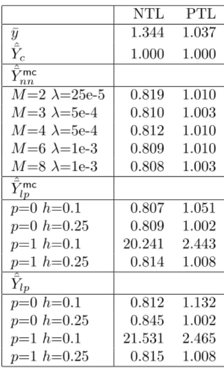
In this section we report on some simulation experiments carried on to investigate the finite sample per-formance of the proposed estimators of ¯Y. To allow comparisons the design and the structure of this investigation is taken from the simulation study conducted by Breidt and Opsomer (2000) where a single auxiliary variable is considered. Nevertheless, some features have also been changed and introduced to pro-vide new insights into the topic. The simulation studies compare the behavior of the following estimators of

¯ Y: ˆ ¯ Y Horvitz-Thompson ˆ ¯

Yc Calibration-Linear Regression equation (2) ˆ

¯ Ymc

nn Neural Network Model Calibration equation (13) ˆ

¯

Ylp Local Polynomial Regression equation (6) ˆ

¯ Ymc

lp Local Polynomial Model Calibration equation (21).

The first two estimators are parametric estimators, in that they assume, respectively, a constant and a linear model for the regression function of the survey variable. The other estimators allow for more complex modelling of the regression function.

Nonparametric estimators can be considered as classes of estimators, because they all depend on the values taken by different model selection parameters. Namely, the local polynomial estimators depend on the order of the local expansion, on the choice of the kernel functionKand of values taken by the bandwidth hin equation (5). On the other hand, neural network estimators depend on the number of units in the hidden layerM and the weight decay parameterλ, as shown in equations (8) and (12). As these parameters range over their allowed values, different estimators of the mean are generated.

We consider model selection in a pre-sampling perspective. That is, the values of these parameters are determined in advance and kept fixed in repeated sampling. For local polynomial estimators we adopted the choices made by Breidt and Opsomer (2000); more precisely, the local constant and the local linear estimator have been considered. Moreover, the Epanechninkov kernel defined as

K(t) =        0.75(1−t2) if|t|<1 0 otherwise

has been used for all kernel based estimators. The same two different bandwidth values have been considered: h= 0.1 andh= 0.25. Higher order polynomials, such as local quadratic or local cubic approximations, have not been considered: although they provide a smoother approximation for internal points, they pay the price of a far more erratic behavior on the boundaries and in presence of extreme values.

As well as the bandwidth selection for local polynomials, the choice of the complexity parameters for neural networks has always been a challenging issue. To better understand the behavior of neural networks in this particular setting of model calibration, the complexity parameters have been chosen in order to have quite a wide range of possible scenarios; that is we allowedλandM to take different combination of values to investigate their influence on the efficiency of the resulting estimator. In the present work we will report only on five of them to make reporting more tractable. Detailed results are available from the authors. The chosen five combinations of values ofλ andM are not the ones that give the best estimators. Choice has been made in order to have a ‘representative sample’ of them. Namely, we will report on estimators calculated by setting: M = 2 and λ = 25e-5; M = 3 and λ = 5e-4; M = 4 and λ = 5e-4; M = 6 and λ= 1e-3;M = 8 andλ= 1e-3. We will see that the latter two choices provide good results for very different populations as far as a single auxiliary variable is employed. Values ofM greater than 8 provide estimators whose performance is virtually the same as when M = 8 is employed, λkept constant. Values ofλ larger than 1e-3, for these nets provide the same results as having a small value for bothM andλ, therefore are not reported. Neural networks have been actually fitted by means of the R functionnnet(), which employs a quasi-Newton optimizer. Other free and commercial software packages are available. The activation function has been chosen to be logistic.

Survey variables have been generated according to eight different models. Each model is characterized by a univariate regression function, or ‘signal’. That is,Eξ(yk|x) =fk(x), for k = 1, . . . ,8, where x∈ R. We considered the following regression functions:

Linear: f1(x) = 1 + 2(x−0.5),

Quadratic: f2(x) = 1 + 2(x−0.5)2,

Bump: f3(x) = 1 + 2(x−0.5) + exp(−200(x−0.5)2),

Jump: f4(x) = 1 + 2(x−0.5)I(x≤0.65) + 0.65I(x >0.65),

CdF: f5(x) = Φ((0.5−2x)/0.02), where Φ is the standard normal CdF

Exponential: f6(x) = exp(−8x),

Cycle1: f7(x) = 2 + sin(2πx),

Cycle4: f8(x) = 2 + sin(8πx),

withx∈[0,1]. See Breidt and Opsomer (2000) for a discussion on the choice of such signals.

In Breidt and Opsomer (2000) the population values forxare generated as independent and identically distributed uniform on [0,1] random variables. We considered this scenario and a skewed distribution for x as well. That is, we also conducted simulations for which the auxiliary variable is i.i.d. from a Beta distribution with expected value 2/7 and variance 7/196.

The population values for all the survey variables but the fifth one have been generated from the regres-sion functions by adding zero mean normal errors with variance such that the signal to noise ratio would approximately equal four to one for all populations. This implies that approximately 20% of the variance of the survey variables is due to the error. The CdF population, on the contrary, consists of binary mea-surements generated from the linear population in the following way: y5i =I(y1i ≤0.5). Hence, the finite population mean of y5 is the population CdF of y1 at the point t = 0.5. The use of the same estimation

strategy for continuous survey variables and for a binary one could be debatable. Even though more suitable networks can be chosen to account for a binary response, we will employ the same one for all populations to allow comparisons.

The effective value of the proportion of variance due to noise is defined as

VP= S 2 y−Sf2 S2 y , (27)

where S2

y is the population variance of the survey variable and Sf2 is the population variance of the corre-sponding signal.

For each simulation, 1000 samples of size n = 100 have been drawn by simple random sampling from a population of sizeN = 1000, and the estimators calculated together with their variance estimators. The performance of the estimators is evaluated by the following quantities calculated for each estimator:

• Relative Bias of an estimator: RelB( ˆY¯∗) = (E( ˆb Y¯∗)−Y¯)/Y ,¯ whereEbdenotes the Monte Carlo estimate

of the expected value.

• Scaled Mean Squared Error defined as follows:

SM SE( ˆY¯∗) =

\

M SE( ˆ¯Y∗)

\

M SE(¯y)VP, (28)

where M SE\ is the Monte Carlo estimate of the mean squared error and ¯y is the sample mean, i.e. the Horvitz-Thompson estimator for this design. That is, we compare the mean squared error of an estimator with its lowest possible value. In fact the M SE of the sample mean times the proportion of variance of y due to noise can be considered as the mean squared error of an ideal estimator that perfectly captures the behavior of the signal, and whose left variation is only due to the irreducible error of the noise. Hence, the smaller the value taken by SM SE is, the larger the efficiency of the estimator.

• Relative Bias of a variance estimator: RelB(v( ˆY¯∗)) =

h b

E(v( ˆ¯Y∗))−M SE( ˆ¯\ Y∗)

i

/M SE( ˆ¯\ Y∗).

We first report on the study dealing with the auxiliary variable xgenerated from a uniform distribution, and then move to the one based on a skewed variablexgenerated from a beta distribution.

6.1

Simulation with a Uniform

x

Results for theSM SE of the estimators in this simulation are reported in Table 1. Moreover, the first row of Table 1 shows the values taken by VPfor all populations. Attention will be focused on the behavior of the class of nonparametric estimators rather than on a single estimator. That is, we are interested in the efficiency of the class of estimators, irrespective of the choice of the complexity parameters. It is well known that nonparametric methods are usually sensible to the choice of such parameters, different values of which

may lead to very different fitted values. Since model selection may not be feasibly conducted for all survey variables, when more than one is of concern, understanding the behavior of the estimators for a range of values of the complexity parameters is of interest.

Some interesting features arise from this table. First of all, neural network estimators all behave similarly with respect to the choice of the number of units in the hidden layer. On the contrary, estimators based on local polynomials are much more erratic in correspondence of different values of the bandwidth and of the order of the local fit.

Secondly, nonparametric estimators lead to good gains in efficiency with respect to the regression esti-mator in all populations but the linear one. Gains in efficiency of the nonparametric estiesti-mators over the regression estimator are non ignorable and vary with the complexity of the regression function. The values of SM SE for the best nonparametric model calibration estimators are always extremely close to one for most populations. The last population is worth a comment. In this case the regression function is extremely complex (a sinusoid completing four full cycles on [0,1]) and performance of the nonparametric estimators varies widely. This is true even for neural network estimators which usually show a common behavior. The more the complexity parameters allow to approximate more complex functions, the larger the gain in effi-ciency. For neural networks this is clearly shown by the decrease inSM SE with increasing ofM. The same is true for local polynomials with a smaller bandwidth.

Last two columns in Table 1 give an indication when ‘robustness’ over different populations is of interest. Namely, the last column reports the average value of SM SE over all populations. We see that the last population is somehow peculiar and determines sometimes a large part of the gain in efficiency for the estimator with a more complex underlying nonparametric method. Hence, in the last but one column we report the same average after removing the last population.

Local polynomial model calibration estimators are on average always more efficient than the corresponding local polynomial regression estimators. As expected, gains in efficiency are shown especially when fitted values are obtained with a large value of the bandwidth and/or with a local constant fit. However, all of the neural network estimators are almost always more efficient than the others. This is true for both averages, but, when the last population is inserted, this higher efficiency relatively increases its magnitude for the estimators with a large number of units in the hidden layer. In fact most of the fitted values averaged

over repeated sampling obtained with neural networks are indistinguishable from the real mean function. Differences are shown only for the last population, for which the fit obtained with a small value of M is not able to capture the complexity of the mean function. The situation is different for local polynomials. Averaged fitted values are usually less behaved and even with a small value of the bandwidth they cannot completely capture the patterns of the last population. Further details are available from the authors.

For all cases in this simulation, the relative biases were less than one percent for all estimators of the population mean, and are therefore not presented. This is not true for the relative biases of the variance estimators which show some interesting patterns. In most cases, variance estimators underestimate the Monte Carlo mean squared error, especially when the nonparametric method overfits the data. In fact, since the estimators of the variance are all based on the residuals from the fitted values, the harder the nonparametric method fits the data, the smaller the residuals and hence the variance estimator, and the smaller the generalization power and hence the larger the mean squared error. The relative bias ranges from 6% to 23% for most populations, with the exception of the Cycle4 population, for which the relative bias increases up to 30% and of the Linear population for which overestimation of the mean squared error is observed. Sample sizes larger than the one considered here are likely required to reduce the underestimation of the variance estimator.

6.2

Simulation with a Skewed

x

Population values for the auxiliary variable in this simulation have been generated from the beta distribution previously introduced. Results for the SM SE of the estimators are reported in Table 2, together with the values taken by VPfor all populations. Relative biases of all estimators are again negligible taking values less than one percent in all cases.

In this case differences are more striking. Neural network estimators perform rather well across all populations with a small degree of variability over the different values of M and λ. Their SM SE takes values close to one for most populations. Exceptions are only observed for the Cycle4 population. On the other hand, the efficiency of local polynomial estimators varies widely across populations and show large losses in efficiency in several cases. This is particularly true when we calculate fitted values by means of a local linear fit and a small bandwidth. The performance of ˆY¯lp and ˆY¯lpmc in this case is quite poor for

all populations. This may be explained by the fact that with this positively skewed distribution there is a boundary of the support of x, and consequently of the survey variables, which is less densely populated. Hence, there are samples for which points on the boundary do not provide a reasonable local approximation when the bandwidth is too small. Further, the additional regression step performed by ˆ¯Ymc

lp with respect to ˆ¯

Ylpdetermines, in this case, an improvement in efficiency. This is particularly true again for cases in which the approximating power of the underlying method is not sufficient to properly fit the data. In particular, increases in efficiency are shown in correspondence of a local constant fit with a large bandwidth.

Variance estimators are again negatively biased in all populations but the linear one. Relative bias usually takes values ranging from 5% to 24%, with a large value for the Cycle4 population of about 43%. This relatively poor performance suggests that further investigation of variance estimation is needed for particularly complex regression functions.

7

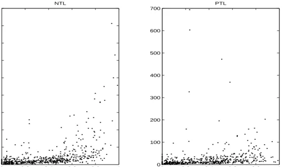
The Mid-Atlantic Highlands region includes the area from the Blue Ridge Mountains in the east to the Ohio River in the west and from the Catskill Mountains in the north to North Carolina in the south. In the years 1993-1996 more than 500 stream reaches across this region have been sampled, visited and some of them re-visited to assess their condition in terms of the chemistry and the health of the biological organisms of the stream (EPA, 2000). Among the factors affecting the condition of the streams, high concentrations of nitrogen and of phosphorus are symptoms of excessive nutrients introduced into the stream. This phenomenon would likely increase algal growth, thereby depleting the oxygen in the water, choking out other forms of biota and significantly altering the animal communities present. One possible cause of nutrient enrichment to streams can be found in agricultural fertilizer application to fields. The proportion of land devoted to agriculture in a particular watershed can be obtained from remote sensing, and would therefore be available for all stream locations without going on site. A square root transformation of this independent variable will overcome the problem of concentration of points on small values. Figure 2 shows the scatterplots of the Total Nitrogen (NTL) and Total Phosphorus (PTL) concentrations, respectively, with respect to the square root of the proportion of Agricultural land (AG) for 574 streams. Only the first visit for each stream has been considered. In spite of the presence of numerous influential observations, a linear regression model

would seem adequate for the relation of PTL with AG. On the other hand, a more complex structure for the relation of NTL with AG might be be considered. To investigate whether nonparametric model calibration could be of use in such a context, we conducted a simulation study. In particular, we considered the set of N = 574 streams as a finite population for which NTL and PTL are survey variables of interest. Moreover, AG can be considered as an auxiliary variable whose value is available for each unit in the population from remote sensing. For each survey variable we selected 1000 random samples without replacement ofn= 100 units. For each sample the same set of estimators considered in the previous section has been calculated and their performance evaluated. Since the true mean function in the relation between the survey variables and the auxiliary variable is unknown, the relative efficiency of the estimators is defined to be

Ef f( ˆY¯∗) = \ M SE( ˆ¯Y∗) \ M SE( ˆY¯c) , (29)

where, again,M SE\is the Monte Carlo estimate of the mean squared error and ˆ¯Ycis the calibration estimator in (2).

Table 3 shows the values of the efficiency for both survey variables. Good gains in efficiency with respect to the calibration estimator are provided for NTL by all neural network estimators almost independently on the choice of the complexity parameters. Moreover, negligible losses of efficiency are shown for PTL. On the other hand, the local polynomial model calibration estimator is usually more efficient than the local polynomial regression estimator and provides the same good performance as that of neural networks in all cases but one. When fitted values are obtained by means of a local linear fit with a small bandwidth, the performance of the resulting estimators is really poor. This behavior can be explained by the presence of extreme points which, when sampled and considered in a local linear fit with few observations, provide unreasonable approximations. The model calibration estimator does not perform much better than local polynomial regression one, since inefficiency in this situation is provided by overfitting the data. This problem is overcome by kernel approximations by means of a more robust local constant fit. Therefore, when irregular data is considered and a local approximation is to be performed, it is preferable to obtain fitted values with a more biased, but at the same time more robust approximator, and then perform the calibration step to recover efficiency.

8

We have proposed and studied an application of nonparametric methods to the model calibration approach introduced by Wu and Sitter (2001) to the use of complete auxiliary information in complex surveys to estimate totals and means. The original idea of model calibration involves fitting a general working model - a nonlinear model or a generalized linear model - and then calibrating on the resulting fitted values as opposed to on the auxiliary variables themselves as proposed for classical calibration.

Our application allows more flexible modelling by assuming more general models and employs nonpara-metric methods to obtain the fitted values to calibrate on. More precisely, we adopt neural network learning and local polynomial smoothing to estimate the functional relationship between the survey variable and the auxiliary variables. The resulting estimates are defined in order to account for the sampling design: this allows deriving design consistent estimators.

The performance of the proposed estimators for finite size samples has been investigated by means of two simulation studies. We compare nonparametric model calibration estimators with nonparametric regression estimators and classical parametric ones and explore the effects of different distributions of the survey variables. Gains in efficiency with respect to the classical regression estimator are provided in all cases by neural network estimators, except when sampling from a linear population. Another important pattern shown by neural networks is that, once a weight decay parameter is included in the learning procedure, fitted values calculated by means of a different number of units in the hidden layer - M ranging from 2 to 8 -provide estimators which display very similar behaviors. This is an interesting robustness result that puts less concern on model selection for neural networks. That is, once weight decay penalization is employed, choice of the number of units in the hidden layer is less important and does not imply in any case particularly erratic results. Different performances are shown only when approximating extremely complex functions.

The above findings also provide quite a general rule to increase efficiency. Namely, insert a reasonable large number of units in the hidden layer to provide good performance on complex functions. Then tune the weight decay parameter to provide good results and avoid losses of efficiency when estimating means of survey variables with a non complex structure. In this way, if more than one survey variable is of concern and model selection cannot be conducted efficiently for each variable, neural networks show good performances

even if the same structure is employed for all of them.

On the other hand, local polynomial estimators are much more sensible to the choice of the bandwidth value and of the type of local approximation. Efficiency of the resulting estimators varies widely according to the selected values of the complexity parameters. Hence, performance of such estimators is particularly connected to the approximating properties of the underlying smoothing technique. The same structure may not be efficient enough for all of the survey variables, by this leading to poor robustness. However, in most cases the local polynomial model calibration estimator has shown to be more efficient than the corresponding local polynomial regression estimator. This is particularly true when fitted values are biased because obtained with a technique that underfits the data: the calibration step performed by the model calibration estimator in these cases recover the efficiency lost by the approximating technique.

Further empirical investigation is needed to explore the behavior of the proposed neural network esti-mator when applied to multivariate auxiliary information. From statistical learning theory and evidence, neural networks would less run into the difficulties generated by the curse of dimensionality if compared to local polynomial smoothing. Nevertheless, their behavior in comparison to estimators based on generalized additive models proposed in literature (Opsomer, Moisen and Kim, 2001) is currently being investigated by the authors.

APPENDIX: PROOFS AND REGULARITY CONDITIONS

Lemma 1. Assume (i)-(vii). Partition the parameter space as in Remark 3 and restrict to Θ1, say. Then

the design based estimator ofθ˜obtained by equation (12) is such that θˆ=θ˜+Op(n−1/2), where subscript 1

is dropped for ease of notation.

Proof. The proof is adapted from Wu (1999), who establishes this lemma for population parameters defined by estimating equations. Firstly, θ˜and θˆare weighted least squares estimates for a nonlinear function f(·). Existence of a solution to both equations (11) and (12) is then guaranteed by continuity of f(·) and compactness of the parameters space (Wu, 1981). Restricting the parameter space to a subset Θ1of Θ built

as in Remark 3, provides uniqueness of bothθ˜andθ. For ease of notation let us rewrite equations (11) andˆ (12) as PN_i=1ζ(yi,xi;θ) = 0and Pin=1diζ(yi,xi;θ) = 0, respectively. Since the functionf(·) is a linear combination of continuous and differentiable functions, it is differentiable to any order and hence, we can

apply a Taylor series expansion toN−1PN i=1ζ(yi,xi;θ) atˆ θˆ=θ. We have˜ N−1 N X i=1 ζ(yi,xi;θ) =ˆ N−1 ( _N X i=1 ∂ζ(yi,xi;θ) ∂θ _θ =˜θ )′ (θˆ−θ) +˜ op(θˆ−θ),˜ (30) sinceN−1PN

i=1ζ(yi,xi;θ) =˜ 0by definition of θ. By assumptions (iii)-(v) and, thus, Remark 2, we have˜ that N−1 n X i=1 diζ(yi,xi;θ) =N−1 N X i=1 ζ(yi,xi;θ) +Op(n−1/2). (31) Since N−1Pn

i=1diζ(yi,xi;θ) =ˆ 0 by definition of θ, equation (31) calculated atˆ θ = θˆ simplifies to N−1PN

i=1ζ(yi,xi;θ) =ˆ Op(n−1/2).Thus, equation (30) can be rewritten as

( N−1 N X i=1 ∂ζ(yi,xi;θ) ∂θ θ=˜θ )′ (θˆ−θ) +˜ op(θˆ−θ) =˜ Op(n−1/2).

Now, by assumption (iii), continuity off(·) and compactness of the support of thexi’s and of the restricted parameters space, N−1 N X i=1 ∂ζ(yi,xi;θ) ∂θ _θ =˜θ =O(1),

and the argument follows.

Lemma 2. Assume (i)-(vii). Partition the parameter space as in Remark 3 and restrict toΘ1, say. Then

N−1 N X i=1 ˆ fi−N−1 n X i=1 difˆi=Op(n−1/2).

Proof: Let us apply a Taylor series expansion to ˆfi=f(xi,θ) atˆ θˆ=θ; we obtain˜

f(xi,θ) =ˆ f(xi,θ) +˜ ∂f(xi,θ) ∂θ _θ =˜θ ′ (θˆ−θ) +˜ op(θˆ−θ).˜

Now, by continuity of the function f and compactness of the support of the xi’s and of the restricted parameter space, we have that

∂f(xi,θ) ∂θ _θ =˜θ =O(1). (32)

Hence, by Lemma 1 we have N−1 N X i=1 ˆ fi =N−1 N X i=1 ˜ fi+Op(n−1/2) (33) and N−1 n X i=1 difˆi=N−1 n X i=1 dif˜i+Op(n−1/2). (34) By assumptions (iii)-(v), we also have N−1PN

i=1f˜i−N−1Pni=1dif˜i =Op(n−1/2).This relation, together

with equations (33) and (34), implies the argument.

Lemma 3. Assume (i)-(vii). Partition the parameter space as in Remark 3 and restrict toΘ1, say. Then

N−1 N X i=1 ˆ fi−N−1 n X i=1 difˆi =N−1 N X i=1 ˜ fi−N−1 n X i=1 dif˜i+Op(n−1).

Proof: A second-order Taylor series expansion off(xi,θ) atˆ θˆ=θ˜is given by

f(xi,θ) =ˆ f(xi,θ) +˜ ∂f(xi,θ) ∂θ _θ =˜θ ′ (θˆ−θ)+˜ +(θˆ−θ)˜′ ∂2_f(x i,θ) ∂θ∂θ′ _θ =˜θ (θˆ−θ) +˜ op(θˆ−θ)˜′(θˆ−θ).˜ Similarly to (32) we have that ∂2_f(x

i,θ)/∂θ∂θ′

_θ

=˜θ=O(1).This statement, together with (32) and Lemma

1 implies that N−1 N X i=1 ˆ fi=N−1 N X i=1 ˜ fi+N−1 ( _N X i=1 ∂f(xi,θ) ∂θ _θ =˜θ )′ (θˆ−θ) +˜ Op(n−1) and N−1 n X i=1 difˆi =N−1 n X i=1 dif˜i+N−1 ( _n X i=1 di ∂f(xi,θ) ∂θ _θ =˜θ )′ (θˆ−θ) +˜ Op(n−1). By assumptions (iii)-(v) N−1 (_N X i=1 ∂f(xi,θ) ∂θ _θ =˜θ ) −N−1 ( _n X i=1 di ∂f(xi,θ) ∂θ _θ =˜θ ) =Op(n−1/2).

Lemma 4. Assume (i)-(vii). Partition the parameter space as in Remark 3 and restrict toΘ1, say. Then

ˆ

βnn= ˜βnn+Op(n−1/2).

Proof. We can rewrite ˜βnn as

˜ βnn= N−1PN i=1qif˜iyi−N−1PNi=1qif¯Y¯ N−1PN i=1qif˜i2−N−1 PN i=1qif¯2 and ˆβnnas ˆ βnn= N−1Pn i=1diqifˆiyi−N−1 Pn i=1diqif˘y˘ N−1Pn i=1diqifˆi2−N−1 Pn i=1diqif˘2 .

Hence, ˜βnn can be seen as a function of population means. Namely, ift1 =PN_i=1qif˜iyi, t2 =PN_i=1qif¯Y¯, t3 = PN_i=1qif˜i2 and t4 = PN_i=1qif¯2, then, ˜βnn = ψ(N−1t), where t = {tl}4_l=1. From Lemma 1 we can consider ˆβnn=ψ(N−1ˆt), where ˆt=

_ˆ

tl

4

l=1, and ˆtl is the corresponding estimator oftl, forl= 1, . . . ,4.

Using a first order Taylor approximation we have

ˆ βnn= ˜βnn+ ( ∂ψ ∂(N−1_ˆt) N−1_ˆt_=N−1t )′ (N−1_ˆ t−N−1_{t) +o} p(N−1ˆt−N−1t). (35) Now, for assumptions (iii)-(v) and Lemma 2,N−1_ˆt

1=N−1t1+Op(n−1/2).Since ˘f and ˘yare ratio estimators, both ˘f = ¯f +Op(n−1/2) and ˘y = ¯Y +Op(n−1/2) hold. Hence, N−1ˆt2 =N−1t2+Op(n−1/2) and N−1tˆ4=

N−1_t

4+Op(n−1/2).

A first-order Taylor series expansion off2(xi,θ) atˆ θˆ=θ˜is given by

f2(xi,θ) =ˆ f2(xi,θ) + 2˜ f(xi,θ)˜ ∂f(xi,θ) ∂θ _θ =˜θ ′ (θˆ−θ) +˜ op(θˆ−θ).˜

For continuity off(·) and compactness of the support of thexi’s and of the restricted parameters space and for equation (32), N−1 N X i=1 f(xi,θ)˜ ∂f(xi,θ) ∂θ _θ =˜θ =O(1);

hence, following the same procedure of Lemma 2 we can state thatN−1_ˆt

Sinceψ(N−1_{t) is a continuous function of bounded quantities, each partial derivative is bounded.}

Com-bining this in equation (35) with the relationships between the population totalstl, forl= 1, . . . ,4, and the

corresponding estimators ˆtl, the argument follows.

Proof of Theorem 1.

1. Design Consistency. Let us consider the estimator introduced in equation (17). Being a generalized differ-ence type estimator, it is unbiased and consistent for ¯Y for assumptions (iii)−(v). Now, ˆ¯Ymc

nn converges in probability to ˜Y¯mc

nn since, by Lemma 4 and Lemma 3, we can rewrite ˆ¯Y mc nn as ˆ ¯ Ymc nn = ˆY¯+ ( N−1 N X i=1 ˜ fi−N−1 n X i=1 dif˜i ) ˜ βnn+Op(n−1) = ˜¯Ynnmc+Op(n−1). (36) Therefore, ˆY¯mc

nn converges in probability to ¯Y and the argument follows.

2. Asymptotic Normality. Convergence in probability implies convergence in distribution, therefore ˆ¯Ymc nn inherits the limiting distribution of ˜Y¯mc

nn. A central limit theorem can be established for ˜¯Y mc nn from

assumptions (iii)−(v) and the result is established.

Proof of Theorem 2.

Being the design variance of the Horvitz-Thompson estimator of the mean of the population residualsEi, we have that V( ˜¯Ymc

nn) =O(n−1). Hence, it suffices to show thatv( ˆ¯Y mc

nn)−V( ˜¯Y mc

nn) =op(n−1). Let us consider the following estimator ofV( ˜Y¯mc

nn): v( ˜Y¯mc nn) = 1 N2 n X i n X j πij−πiπj πij Ei πi Ej πj . From assumption (v), v( ˜Y¯mc nn)−V( ˜Y¯ mc

nn) =op(n−1). Now, since eiej =EiEj+Op(n−1/2) by Lemma 4 and the fact that ˆfi = ˜fi+Op(n−1/2) from Lemma 2,v( ˆY¯nnmc) =v( ˜¯Y

mc

nn) +op(n−3/2) and the argument follows.

Regularity conditions for Theorem 3.

(A1) For eachν, thexi, fori = 1, . . . , N, are independent and identically distributed F(x) =R_−∞x g(t)dt, where g(·) is a density with compact support [ax, bx] and g(x)>0 for allx∈[ax, bx].