A deep matrix factorization method for learning
attribute representations
George Trigeorgis, Konstantinos Bousmalis,
Student Member, IEEE,
Stefanos Zafeiriou,
Member, IEEE
Bj ¨orn W. Schuller,
Senior member, IEEE
Abstract—Semi-Non-negative Matrix Factorization is a technique that learns a low-dimensional representation of a dataset that lends itself to a clustering interpretation. It is possible that the mapping between this new representation and our original data matrix contains rather complex hierarchical information with implicit lower-level hidden attributes, that classical one level clustering methodologies can not interpret. In this work we propose a novel model, Deep Semi-NMF, that is able to learn such hidden representations that allow themselves to an interpretation of clustering according to different, unknown attributes of a given dataset. We also present a semi-supervised version of the algorithm, named Deep WSF, that allows the use of (partial) prior information for each of the known attributes of a dataset, that allows the model to be used on datasets with mixed attribute knowledge. Finally, we show that our models are able to learn low-dimensional representations that are better suited for clustering, but also classification, outperforming Semi-Non-negative Matrix Factorization, but also other state-of-the-art methodologies variants.
Index Terms—Semi-NMF, Deep Semi-NMF, unsupervised feature learning, face clustering, semi-supervised learning, Deep WSF, WSF, matrix factorization, face classification
F
1
INTRODUCTION
M
ATRIXfactorization is a particularly useful family of techniques in data analysis. In recent years, there has been a significant amount of research on factor-ization methods that focus on particular characteristics of both the data matrix and the resulting factors. Non-negative matrix factorization (NMF), for example, fo-cuses on the decomposition of non-negative multivariate data matrix X into factors Z and H that are also non-negative, such that X ≈ ZH. The application area of the family of NMF algorithms has grown significantly during the past years. It has been shown that they can be a successful dimensionality reduction technique over a variety of areas including, but not limited to, environ-metrics [1], microarray data analysis [2], [3], document clustering [4], face recognition [5], [6], blind audio source separation [7] and more. What makes NMF algorithms particularly attractive is the non-negativity constraints imposed on the factors they produce, allowing for better interpretability. Moreover, it has been shown that NMF variants (such as the Semi-NMF) are equivalent to a soft version of k-means clustering, and that in fact, NMF variants are expected to perform better than k-means clustering particularly when the data is not distributed in a spherical manner [8], [9].In order to extend the applicability of NMF in cases where our data matrix X is not strictly non-negative, [8] introduced Semi-NMF, an NMF variant that imposes • G. Trigeorgis, S. Zafeiriou, and B. W. Schuller are with the Department
of Computing, Imperial College London, SW7 2RH, London, UK E-mail:[email protected]
• K. Bousmalis is with Google Robotics E-mail:[email protected]
non-negativity constraints only on the second factor
H, but allows mixed signs in both the data matrix
X and the first factor Z. This was motivated from a clustering perspective, where Z represents cluster cen-troids, and H represents soft membership indicators for every data point, allowing Semi-NMF to learn new lower-dimensional features from the data that have a convenient clustering interpretation.
It is possible that the mapping Z between this new representation H and our original data matrix X con-tains rather complex hierarchical and structural informa-tion. Such a complex datasetX is produced by a multi-modal data distribution which is a mixture of several distributions, where each of these constitutes anattribute of the dataset. Consider for example the problem of mapping images of faces to their identities: a face image also contains information about attributes like pose and expression that can help identify the person depicted. One could argue that by further factorizing this mapping
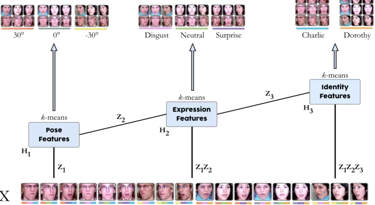
Z, in a way that each factor adds an extra layer of abstraction, one could automatically learn such latent at-tributes and the intermediate hidden representations that are implied, allowing for a better higher-level feature representationH. In this work, we propose Deep Semi-NMF, a novel approach that is able to factorize a matrix into multiple factors in an unsupervised fashion – see Figure 1, and it is therefore able to learn multiple hidden representations of the original data. As Semi-NMF has a close relation to k-means clustering, Deep Semi-NMF also has a clustering interpretation according to the different latent attributes of our dataset, as demonstrated
in Figure 2. Using a non-linear deep model for matrix
factorization also allows us to project data-points which are not initially linearly separable into a representation
X H Z (a) Semi-NMF X H1 · · · Hm Z1 Z2 Zm (b) Deep Semi-NMF Fig. 1. (a) A Semi-NMF model results in a linear trans-formation of the initial input space. (b) Deep Semi-NMF learns a hierarchy of hidden representations that aid in uncovering the final lower-dimensional representation of the data.
that is; fact which we demonstrate in subsection 6.1. It might be the case that the different attributes of our data are not latent. If those are known and we actually have some label information about some or all of our data, we would naturally want to leverage it and learn representations that would make the data more separa-ble according to each of these attributes. To this effect, we also propose a weakly-supervised Deep Semi-NMF (Deep WSF), a technique that is able to learn, in a semi-supervised manner, a hierarchy of representations for a given dataset. Each level of this hierarchy corresponds to a specific attribute that is known a priori, and we show that by incorporating partial label information via graph regularization techniques we are able to perform better than with a fully unsupervised Deep Semi-NMF in the task of classifying our dataset of faces according to different attributes, when those are known. We also show that by initializing an unsupervised Deep
Semi-NMF with the weights learned by a Deep WSF we
are able to improve the clustering performance of the Deep Semi-NMF . This could be particularly useful if we have, as in our example, a small dataset of images of faces with partial attribute labels and a larger one with no attribute labels. By initializing a Deep Semi-NMF with the weights learned with Deep WSF from the small labelled dataset we can leverage all the information we have and allow our unsupervised model to uncover better representations for our initial data on the task of clustering faces.
Relevant to our proposal are hierarchical clustering algorithms [10], [11] which are popular in gene and document clustering applications. These algorithms typ-ically abstract the initial data distribution as a form of tree called a dendrogram, which is useful for analysing the data and help identify genes that can be used as biomarkers or topics of a collection of documents. This
makes it hard to incorporate out-of-sample data and prohibits the use of other techniques than clustering.
Another line of work which is related to ours is multi-label learning [12]. Multi-label learning techniques rely on the correlations [13] that exist between different attributes to extract better features. We are not interested in cases where there is complete knowledge about each of the attributes of the dataset but rather we propose a new paradigm of learning representations where have data with only partly annotated attributes. An example of this is a mixture of datasets where each one has label information about a different set of attributes. In this new paradigm we can not leverage the correlations between the attribute labels and we rather rely on the hierarchical structure of the data to uncover relations between the different dataset attributes. To the best of our knowledge this is the first piece of work that tries to automatically discover the representations for different (known and unknown) attributes of a dataset with an application to a multi-modal application such as face clustering.
The novelty of this work can be summarised as fol-lows: (1) we outline a novel deep framework1 for ma-trix factorization suitable for clustering of multimodally distributed objects such as faces,(2)we present a greedy algorithm to optimize the factors of the Semi-NMF prob-lem, inspired by recent advances in deep learning [15], (3) we evaluate the representations learned by different NMF–variants in terms of clustering performance, (4) present the Deep WSF model that can use already known (partial) information for the attributes of our data distri-bution to extract better features for our model, and (5) demonstrate how to improve the performance of Deep Semi-NMF , by using the existing weights from a trained Deep WSF model.
2
BACKGROUND
In this work, we assume that our data is provided in a matrix form X ∈ Rp×n, i.e., X = [x1,x2, . . . ,xn] is
a collection of n data vectors as columns, each with
p features. Matrix factorization aims at finding factors of X that satisfy certain constraints. In Singular Value Decomposition (SVD) [16], the method that underlies Principal Component Analysis (PCA) [17], we factorize
X into two factors: the loadings or bases Z ∈ Rp×k
and the features or components H ∈ Rk×n, without
imposing any sign restrictions on either our data or the resulting factors. In Non-negative Matrix Factorization (NMF) [18] we assume that all matrices involved contain only non-negative elements2, so we try to approximate
a factorizationX+≈Z+H+.
1. A preliminary version of this work has appeared in [14]. 2. When not clear from the context we will use the notationA+to state that a matrixAcontains only non-negative elements. Similarly, when not clear, we will use the notation A± to state thatA may contain any real number.
2.1 Semi-NMF
In turn, Semi-NMF [8] relaxes the non-negativity con-strains of NMF and allows the data matrix X and the loadings matrixZto have mixed signs, while restricting only the features matrix H to comprise of strictly non-negative components, thus approximating the following factorization:
X±≈Z±H+. (1)
This is motivated from a clustering perspective. If we
view Z= [z1,z2, . . . ,zk] as the cluster centroids, then
H= [h1,h2, . . . ,hn] can be viewed as the cluster
indi-cators for each datapoint.
In fact, if we had a matrix H that was not only non-negative but also orthogonal, such that HHT =I [8], then every column vector would have only one positive element, making Semi-NMF equivalent tok-means, with the following cost function:
Ck−means= n X i=1 k X j=1 hkikxi−zkk2=kX−ZHk2F (2)
where k · k denotes the L2-norm of a vector and k · kF
the Frobenius norm of a matrix.
Thus Semi-NMF, which does not impose an orthog-onality constraint on its features matrix, can be seen as a soft clustering method where the features matrix describes the compatibility of each component with a cluster centroid, a base in Z. In fact, the cost function we optimize for approximating the Semi-NMF factors is indeed:
CSemi-NMF=kX−ZHk2F. (3)
We optimize CSemi-NMF via an alternate optimization of Z± and H+: we iteratively update each of the factors while fixing the other, imposing the non-negativity con-strains only on the features matrix H:
Z←XH† (4)
where H† is the Moore–Penrose pseudo-inverse of H, and H←H v u u t [Z>X]pos+ [Z>Z]negH [Z>X]neg+ [Z>Z]posH (5)
where is a small number to avoid division by zero,
Apos is a matrix that has the negative elements of matrix
Areplaced with 0, and similarlyAnegis one that has the positive elements of Areplaced with 0:
∀i, j .Aposij =|Aij|+Aij 2 , A neg ij = | Aij| −Aij 2 . (6) 2.2 State-of-the-art for learning features for cluster-ing based on NMF-variants
In this work, we compare our method with, among others, the state-of-the-art NMF techniques for learning features for the purpose of clustering. [19] proposed a
graph-regularized NMF (GNMF) which takes into ac-count the intrinsic geometric and discriminating struc-ture of the data space, which is essential to the real-world applications, especially in the area of clustering. To accomplish this, GNMF constructs a nearest neighbor graph to model the manifold structure. By preserving the graph structure, it allows the learned features to have more discriminating power than the standard NMF algorithm, in cases that the data are sampled from a submanifold which lies in a higher dimensional ambient space.
Closest to our proposal is recent work that has pre-sented NMF-variants that factorize X into more than 2 factors. Specifically, [20] have demonstrated the concept of Multi-Layer NMF on a set of facial images and [21], [22], [23] have proposed similar NMF models that can be used for Blind Source Separation, classification of digit images (MNIST), and documents. The representations of the Multi-layer NMF however do not lend themselves to a clustering interpretation, as the representations learned from our model. Although the Multi-layer NMF is a promising technique for learning hierarchies of features from data, we show in this work that our proposed model, the Deep Semi-NMF outperforms the Multi-layer NMF and, in fact, all models we compared it with on the task of feature learning for clustering images of faces.
2.3 Semi-supervised matrix factorization
For the case of the proposed Deep WSF algorithms, we also evaluate our method with previous semi-supervised non-negative matrix factorization techniques. These in-clude the Constrained Nonnegative Matrix Factorization (CNMF) [24], and the Discriminant Nonnegative Matrix Factorization (DNMF) [25]. Although both take label information as additional constraints, the difference be-tween these is that CNMF uses the label information as hard constrains on the resulting features H, whereas DNMF tries to use the Fisher Criterion in order to incorporate discriminant information in the decompo-sition [25]. Both approaches only work for cases where we want to encode the prior information of only one attribute, in contrast to the proposed Deep WSF model.
3
DEEP
SEMI-NMF
In Semi-NMF the goal is to construct a low-dimensional representation H+ of our original data X±, with the bases matrix Z± serving as the mapping between our original data and its lower-dimensional representation
(see Equation 1). In many cases the data we wish to
analyze is often rather complex and has a collection of distinct, often unknown, attributes. In this work for example, we deal with datasets of human faces where the variability in the data does not only stem from the difference in the appearance of the subjects, but also from other attributes, such as the pose of the head in relation to the camera, or the facial expression of the subject. The multi-attribute nature of our data calls for a hierarchical
X
30°
0°
-30°
Disgust
Neutral
Surprise
Charlie
Dorothy
Z 1 Z1Z2 Z1Z2Z3
k
-means
k
-means
k
-means
H 1 H 2 H 3 Z 3 Z 2Fig. 2. A Deep Semi-NMF model learns a hierarchical structure of features, with each layer learning a representation suitable for clustering according to the different attributes of our data. In this simplified, for demonstration purposes, example from the CMU Multi-PIE database, a Deep Semi-NMF model is able to simultaneously learn features for pose clustering (H1), for expression clustering (H2), and for identity clustering (H3). Each of the images inXhas an
asso-ciated colour coding that indicates its memberships according to each of these attributes (pose/expression/identity).
framework that is better at representing it than a shallow Semi-NMF.
We therefore propose here the Deep Semi-NMF model, which factorizes a given data matrixXintom+1factors, as follows:
X±≈Z±1Z2±· · ·Z±mH+m (7)
This formulation, as shown directly in Equation 9 with respect to Figures 1 and 2 allows for a hierarchy of m
layers of implicit representations of our data that can be given by the following factorizations:
H+m−1≈Z ± mH + m .. . H+2≈Z±3 · · ·Z±mH+m H+1≈Z ± 2 · · ·Z ± mH + m (8)
As one can see above, we further restrict these implicit representations (H+1, . . . ,H+m−1) to also be non-negative. By doing so, every layer of this hierarchy of representa-tions also lends itself to a clustering interpretation, which constitutes our method radically different to other multi-layer NMF approaches [21], [22], [23]. By examining Figure 2, one can better understand the intuition of how
that happens. In this case the input to the model, X, is a collection of face images from different subjects (identity), expressing a variety of facial expressions taken from many angles (pose). A Semi-NMF model would find a representation H of X, which would be useful for performing clustering according to the identity of the subjects, andZthe mapping between these identities and the face images. A Deep Semi-NMF model also finds a representation of our data that has a similar interpre-tation at the top layer, its last factor Hm. However, the
mapping from identities to face images is now further analyzed as a product of three factors Z=Z1Z2Z3, with Z3 corresponding to the mapping of identities to expressions,Z2Z3 corresponding to the mapping of identities to poses, and finallyZ1Z2Z3corresponding to the mapping of identities to the face images. That means that, as shown in Figure 2 we are able to decompose our data in 3 different ways according to our 3 different attributes:
X±≈Z±1H+1
X±≈Z±1Z±2H+2
X±≈Z±1Z±2Z±3H+3 (9) More over, due to the non-negativity constrains we en-force on the latent featuresH(·), it should be noted that
this model does not collapse to a Semi-NMF model. Our hypothesis is that by further factorizingZwe are able to construct a deep model that is able to (1) automatically learn what this latent hierarchy of attributes is; (2) find representations of the data that are most suitable for clustering according to the attribute that corresponds to each layer in the model; and (3) find a better high-level, final-layer representation for clustering according to the attribute with the lowest variability, in our case the identity of the face depicted. In our example in
Figure 2 we would expect to find better features for
clustering according to identities H+3 by learning the hidden representations at each layer most suitable for each of the attributes in our data, in this example:
H+1 ≈ Z±2Z±3H+3 for clustering our original images in terms of poses andH+2 ≈Z±3H+3 for clustering the face images in terms of expressions.
In order to expedite the approximation of the factors in our model, we pretrain each of the layers to have an initial approximation of the matrices Zi,Hi as this
greatly improves the training time of the model. This is a tactic that has been employed successfully before [15] on deep autoencoder networks. To perform the pre-training, we first decompose the initial data matrix X ≈Z1H1, where Z1 ∈ Rp×k1 and H
1 ∈ R+0
k1×n
. Following this, we decompose the features matrix H1≈Z2H2, where
Z2∈Rk1×k2andH
1∈R+0
k2×n
, continuing to do so until we have pre-trained all of the layers. Afterwards, we can fine-tune the weights of each layer, by employing alternating minimization (with respect to the objective function inEquation 10) of the two factors in each layer, in order to reduce the total reconstruction error of the model, according to the cost function in Equation 10.
Cdeep= 1 2kX−Z1Z2· · ·ZmHmk 2 F =tr[X>X−2X>Z1Z2· · ·ZmHm +H>mZ>mZ>m−1· · ·Z>1Z1Z2· · ·ZmHm] (10)
Update rule for the weights matrix ZWe fix the rest of the weights for theithlayer and we minimize the cost
function with respect to Zi. That is, we set
∂Cdeep
∂Zi
= 0, which gives us the updates:
Zi= (Ψ>Ψ)−1Ψ>XH˜i > ( ˜HiH˜i > )−1 Zi=Ψ†XH˜ † i (11)
where Ψ=Z1· · ·Zi−1, †denotes the Moore-Penrose pseudo-inverse and H˜i is the reconstruction of the ith
layer’s feature matrix.
Update rule for features matrix HUtilizing a similar proof to [8], we can formulate the update rule for Hi
which enforces the non-negativity ofHi:
Hi=Hi s [Ψ>X]pos+ [Ψ>Ψ]negH i [Ψ>X]neg+ [Ψ>Ψ]posH i . (12)
Algorithm 1 Suggested algorithm for training a Deep
Semi-NMF model3. Initially we approximate the factors
greedily using the SEMI-NMF algorithm [8] and we fine-tune the factors until we reach the convergence criterion.
Input:X ∈Rp×n, list of layer sizes
Output:weight matrices Zi and feature matrices Hi
for each of the layers Initialize Layers for alllayersdo
Zi,Hi← SEMINMF(Hi−1, layers(i)) end for
repeat
for alllayersdo
˜ Hi← ( Hi if i=k Zi+1H˜i+1 otherwise Ψ←Qi−1 k=1Zk Zi ←Ψ†XH˜ † i Hi←Hi " [Ψ>X]pos+ [Ψ>Ψ]negH i [Ψ>X]neg+ [Ψ>Ψ]posH i #η end for
untilStopping criterion is reached
Complexity
The computational complexity for the
pre-training stage of Deep Semi-NMF is of order
O mt pnk+nk2+kp2+kn2, wheremis the number
of layers, t the number of iterations until convergence and k is the maximum number of components out of all the layers. The complexity for the fine-tuning stage isO mtf pnk+ (p+n)k2where tf is the number of
additional iterations needed.
3.1 Non-linear Representations
By having a linear decomposition of the initial data distribution we may fail to describe efficiently the non-linearities that exist in between the latent attributes of the model. Introducing non-linear functions between the layers, can enable us to extract features for each of the latent attributes of the model that are non-linearly separable in the initial input space.
This is motivated further from neurophysiology paradigms, as the theoretical and experimental evidence suggests that the human visual system has a hierarchical and rather non-linear approach [26] in processing image structure, in which neurons become selective to pro-cess progressively more complex features of the image structure. As argued by Malo et al. [27], employing an adaptive non-linear image representation algorithm results in a reduction of the statistical and the perceptual redundancy amongst the representation elements.
3. The implementation and documentation ofAlgorithm 1can be found athttp://trigeorgis.com/deepseminmf.
From a mathematical point of view, one can use a non-linear function g(·), between each of the implicit representations (H+1, . . . ,H+m−1), in order to better ap-proximate the non-linear manifolds which the given data matrix X originally lies on. In other words by using a non-linear squashing function we enhance the express-ibility of our model and allow for a better reconstruction of the initial data. This has been proved in [28] by the use of the Stone-Weierstrass theorem, in the case of multilayer feedforward network structures, which Semi-NMF is an instance of, that arbitrary squashing functions can approximate virtually any function of interest to any desired degree of accuracy, provided sufficiently many hidden units are available.
To introduce non-linearities in our model we modify theith feature matrixHi, by setting
Hi≈g(Zi+1Hi+1). (13) which in turns changes the objective function of the model to be:
C∗= 1
2kX−Z1g(Z2g(· · ·g(ZmHm)))k
2
F (14)
In order to compute the derivative for the ith feature
layer, we make use of the chain rule and get:
∂C∗ ∂Hi =Z>i ∂C∗ ∂ZiHi =Z>i ∂C∗ ∂g(ZiHi) ∇ g(ZiHi) =Z>i ∂C∗ ∂Hi−1 ∇ g(ZiHi)
The derivation of the first feature layer H1 is then identical to the version of the model with one layer.
∂C∗ ∂H1 = 1 2 ∂T r[−2X>Z1H1+ (Z1H1)>Z1H1] ∂H1 =Z>1Z1H1−Z>1X =Z>1 (Z1H1−X).
Similarly we can compute the derivative for the weight matrices Zi, ∂C∗ ∂Zi = ∂C ∗ ∂ZiHi H>i = ∂ C∗ ∂g(ZiHi) ∇ g(ZiHi) H>i = ∂C∗ ∂Hi−1 ∇ g(ZiHi) H>i and ∂C∗ ∂Z1 = 1 2 ∂T r[−2X>Z1H˜1+ (Z1H˜1)>Z1H˜1] ∂Z1 =Z1H˜1−X ˜ H>1
Using these derivatives we can make use of gradient descent optimizations such as Nesterov’s optimal gradi-ent [29], to minimize the cost function with respect to each of the weights of our model.
4
W
EAKLY-S
UPERVISEDA
TTRIBUTEL
EARN-ING
As before, consider a dataset of facesXas inFigure 2. In this dataset, we have a collection of subjects, where each one has a number of images expressing different expres-sions, taken by different angles (pose information). A three layer Deep Semi-NMF model could be used here to automatically learn representations in an unsupervised manner (Hpose,Hexpression,Hidentity) that conform to this latent hierarchy of attributes. Of course, the features are extracted without accounting (partially) available information that may exist for each of the these attributes of the dataset.
To this effect we propose a Deep Semi-NMF approach that can incorporate partial attribute information that we named Weakly-Supervised Deep Semi-Nonnegative Matrix Factorization (Deep WSF). Deep WSF is able to learn, in a semi-supervised manner, a hierarchy of representations; each level of this hierarchy correspond-ing to a specific attribute for which we may have only partial labels for. As depicted in Figure 3, we show that by incorporating some label information via graph regularization techniques we are able to do better than the Deep Semi-NMF for classifying faces according to pose, expression, and identity. We also show that by initializing a Deep Semi-NMF with the weights learned by a Deep WSF we are able to improve the performance of the Deep Semi-NMF for the task of clustering faces according to identity.
4.1 Incorporating known attribute information
Consider that we have an undirected graph G with N
nodes, where each of the nodes corresponds to one data point in our initial dataset. A node i is connected to another nodejiff we have a priori knowledge that those samples share the same label, and this edge has a weight
wij.
In the simplest case scenario, we use a binary weight matrixW defined as:
Wij=
(
1 if yi =yj
0 otherwise (15)
Instead one can also choose aradial basis function kernel
Wij = ( exp−kxi−xjk2 2σ2 ifyi =yj 0 otherwise (16)
or adot-product weighting, where
Wij =
( x>
i xj if yi = yj
0 otherwise (17)
Using the graph weight matrix W, we formulate L, which denotes the Graph Laplacian [30] that stores our prior knowledge about the relationship of our samples and is defined as L =D−W, where D is a diagonal matrix whose entries are column (or row, since W is
Graph Laplacian - Lidentity Identity features Dataset Angelina George Unlabelledsamples
Graph Laplacian - Lemotion
Happy Sad
Unlabelledsamples
Surprise
Pose features Emotion features
-30 Degrees
30 Degrees
Hpose
Unlabelledsamples
0 Degrees Graph Laplacian - Lpose
Hidentity
Hemotion
Fig. 3. A weakly-supervised Deep Semi-NMF model uses prior knowledge we have about the attributes of our model to improve the final representation of our data. In this illustration we incorporate information from pose, expression, and identity attributes into the 3 feature layers of our modelHpose,Hexpression, andHidentityrespectively.
symmetric) sums of W, Djj = PkWjk. In order to
control the amount of embedded information in the graph we introduce as in [31], [32], [33], a term R which controls the smoothness of the low dimensional representation. R= N X j,l=1 khj−hlk2Wjl = N X j=1 h>jhjDjj− N X j,l=1 h>jhjWjl =TrH>DH−TrH>W H =TrH>LH (18)
where hi is the low-dimensional features for sample i,
that we obtain from the decomposed model.
Minimizing this termR, we ensure that the euclidean difference between the final level representations of any two data points hi and hj is low when we have prior
knowledge that those samples have a relationship, pro-ducing similar features hi and hj. On the other hand,
when we do not have any expert information about some or even all the class information about an attribute, the term has no influence on the rest of the optimization.
Before deriving the update rules and the algorithm for the multi-layer Deep WSF model, we first show the simpler case of the one layer version, which will come into use for pre-training the model, as Semi-NMF can be used to pre-train the purely unsupervised Deep Semi-NMF. We call this model Weakly Supervised Semi-NMF WSF.
By combining the term Rintroduced in Equation 18, with the cost function of Semi-NMF we obtain the cost function for Weakly-Supervised Factorization (WSF).
CWSF=kX−Z±H+k2F+λTr(H
> LH)
s.t.H≥0. (19) The update rules, but also the algorithm for training a WSF model can be found in the supplementary material. We incorporate the available partial labelled informa-tion for the pose, expression, and identity by forming a graph Laplacian for pose for the first layer (Lpose), expression for the second layer(Lexpression), and identity for the third layer (Lidentity) of the model. We can then tune the regularization parameters λi accordingly for
each of the layers to express the importance of each of these parameters to the Deep WSF model. Using the modified version of our objective functionEquation 20, we can derive theAlgorithm 2.
CDeep WSF= 1 2kX−Z1g(. . . g(ZmHm))k 2 F +1 2 m X i=1 λiTr(H>i LiHi) (20)
In order to compute the derivative for the ith feature
layer, we make use of the chain rule and get:
∂Cdwsf ∂Hi =Z>i ∂Cdeep ∂ZiHi +1 2 λiTr(H>i LiHi) ∂Hi =Z>i ∂ Cdeep ∂Hi−1 ∇ g(ZiHi) +λiLiHi
And the derivation of the first feature layerH1 is then:
∂Cdwsf ∂H1 = ∂Cdeep ∂ZiHi +1 2 λ1Tr(H>1L1H1) ∂H1 =Z>1 (Z1H1−X) +λ1L1H1.
Algorithm 2 Proposed algorithm for training a Deep WSF model. Initially we approximate the factors greedily using WSF or Semi-NMF and we fine-tune the factors until we reach the convergence criterion.
Input: X∈Rp×n, list of layer sizeslayers
Output: weight matricesZi and feature matrices Hi
for each of the layers Initialize Layers for all layersdo
Zi,Hi ←WSF(Hi−1, layers(i),λi)
end for repeat
for all layersdo
˜ Hi← ( Hi if i=k Zi+1H˜i+1 otherwise Ψ←Qi−1 k=1Zk Zi←Ψ†XH˜ † i F ← [Ψ >X]pos+ [Ψ>Ψ]negH i+λiHiWi [Ψ>X]neg+ [Ψ>Ψ]posH i+λiHiDi Hi←HiFη end for
until Stopping criterion is reached
Similarly we can compute the derivative for the weight matrices Zi, ∂Cdwsf ∂Zi = ∂Cdeep ∂ZiHi H>i = ∂ Cdeep ∂Hi−1 ∇ g(ZiHi) H>i and ∂Cdwsf ∂Z1 = ∂Cdeep ∂Z1 =Z1H˜1−X ˜ H>1
Using these derivatives we can make use of gradient descent optimizations as with the non-linear Deep Semi-NMF model, to minimize the cost function with respect to each of the factors of our model. If instead use the linear version of the algorithm where g is the identity function, then we can derive a multiplicative update algorithm version of Deep WSF, as described in Algo-rithm 2.
4.2 Weakly Supervised Factorization with Multiple Label Constraints
Another approach we propose within this framework is a single–layer WSF model that learns only a single representation based on information from multiple at-tributes. This Multiple-Attribute extension of the WSF, the WSF-MA, accounts for the case of having multiple number of attributesξfor our data matrixX, by having
a regularization termλiTr[HLiH>]. This term uses the
prior information from all the available attributes to construct ξ Laplacian graphs where each of them has a different regularization factorλi.
This constitutes WSF-MA, whose cost function is
Cmawsf=kX−ZHk2 F + ξ X i=1 λiTr(H>LiH) s.t.H≥0 (21)
The update rules used, and the algorithm can be found in the supplementary material.
5
OUT-OF-SAMPLE PROJECTION
After learning an internal model of the data, either using the purely unsupervised Deep Semi-NMF or to perform semi-supervised learning using the Deep WSF model with learned weightsZ, and featuresHwe can project an out-of-sample data point x∗ to the new
lower-dimensional embedding h∗. We can accomplish this using one of the two presented methods.
METHOD1: BASIS MATRIX RECONSTRUCTION.
Each testing samplex∗ is projected into the linear space
defined by the weights matrixZ. Although this method has been used by various previous works [34], [35] using the NMF model, it doesnotguarantee the non-negativity ofh∗.
For the linear case of Deep WSF, this would lead to
h∗≈[Z1Z2. . .Zl]†x∗. (22)
and for the non-linear case
h∗≈g−1Zl†· · ·Z†2g−1
Z†1x∗
(23) METHOD2: USING NON-NEGATIVITY UPDATE RULES.
Using the same process as in Deep Semi-NMF , we can intuitively learn the new features h∗, by assuming that the weight matrices∀i.Zi remain fixed.
∀l.h∗l = argminhkx∗− l Y i=1 Zihlk (24) such thathl≥0.
and for the non-linear case
∀l.h∗l = argminhkx∗−Z1g(Z2· · ·g(Zlhl))k (25)
such thathl≥0.
where hl, corresponds to the lth feature layer for the
out-of-sample data pointx∗. This problem is then solved
by using Algorithm 1 as Deep Semi-NMF, but without updating the weight matricesZi.
6
E
XPERIMENTSOur main hypothesis is that a Deep Semi-NMF is able to learn better high-level representations of our original data than a one-layer Semi-NMF for clustering according to the attribute with the lowest variability in the dataset. In order to evaluate this hypothesis, we have compared the performance of Deep Semi-NMF with that of other methods, on the task of clustering images of faces in two distinct datasets. These datasets are:
• CMU PIE: We used a freely available version of
CMU Pie [36], which comprises of2,856 grayscale
32×32face images of 68 subjects. Each person has 42 facial images under different light and illumina-tion condiillumina-tions. In this database we only know the identity of the face in each image.
• XM2VTS: The Extended Multi Modal Verification
for Teleservices and Security applications (XM2VTS) [37] contains 2,360 frontal images of 295 different subjects. Each subject has two available images for each of the four different laboratory sessions, for a total of 8 images. The images were eye-aligned and resized to 42×30.
In order to evaluate the performance of our Deep Semi-NMF model, we compared it against not only Semi-NMF [8], but also against other NMF variants that could be useful in learning such representations. More specifically, for each of our two datasets we performed the following experiments:
• Pixel Intensities: By using only the pixel intensities
of the images in each of our datasets, which of course give us a strictly non-negative input data matrixX, we compare the reconstruction error and the clustering performance of our Deep Semi-NMF method against the Semi-NMF, NMF with multi-plicative update rules [18], Multi-Layer NMF [23], GNMF [19], and NeNMF [38].
• Image Gradient Orientations (IGO): In general,
the trend in Computer Vision is to use complicated engineered features like HoGs, SIFT, LBPs, etc. As a proof of concept, we choose to conduct experiments with simple gradient orientations [39] as features, instead of pixel intensities, which results into a data matrix of mixed signs, and expect that we can learn better data representations for clustering faces according to identities. In this case, we only compared our Deep Semi-NMF with its one-layer Semi-NMF equivalent, as the other techniques are not able to deal with mixed-sign matrices.
In subsection 6.6, having demonstrated the
effective-ness of the purely unsupervised Deep Semi-NMF model
we show next how pretraining a Deep WSF model
on an auxiliary dataset and using the learned weights
to perform unsupervised Deep Semi-NMF can lead
to significant improvements in terms of the clustering accuracy.
Finally, in subsection 6.7, we examine the classifi-cation abilities of the proposed models for each of
the three attributes of the CMU Multi-PIE dataset (pose/expression/identity) and use this to test more on our secondary hypothesis, i.e. that every representation in each layer is in fact most suited for learning according to the attributes that corresponds to the layer of interest.
6.1 An example with multi-modal synthetic data
As previously mentioned images of faces are multi-modal distributions which are composed of multiple at-tributes such as pose and identity. A simplified example of such dataset is Figure 4where we have two subjects depicting two poses each. This example two-dimensional dataset XXOR was generated using 100 samples from four normal distributions withσ= 1.
As previously discussed insubsection 3.1, Semi-NMF is an instance of a single layer neural network. As such there can not exist a linear projectionZXOR which maps the original data distributionXXORinto a sub-space such
as the two subjects (red and blue) of the dataset are linearly separable.
Pose #1/Subject #1 Pose #2/Subject #2
Pose #1/Subject #2 Pose #2/Subject #1
Fig. 4. Visualisation ofXXOR, where (+) are samples of
Subject #1 (Subject #2) and red (blue) data points denote the samples of each subject with Pose #1 (Pose #2).
Instead by employing a deep factorization model us-ing the labels for the pose and identity for the first and second layer respectively we can find a non-linear mapping which separates the two identities as shown in Figure 5.
6.2 Implementation Details
To initiate the matrix factorization process, NMF and Semi-NMF algorithms start from some initial point (Z0,H0), where usually Z0 and H0 are randomly ini-tialized matrices.
A problem with this approach, is not only the initial-ization point is far from the final convergence point, but also makes the process non deterministic.
The proposed initialization of Semi-NMF by its au-thors is instead by using the k-means algorithm [40]. Nonetheless, k-means is computationally heavy when the number of components k is fairly high (k > 100). As an alternative we implemented the approach by [41] which suggests exact and heuristic algorithms which
(a) Layer #1 featuresH1 (b) Layer #2 featuresH2
Fig. 5. The features extracted by each of the layers of a deep factorization model on the artificially generated dataset. The second layer manages to find a projection of the initial data which makes all the classes linearly separable, a task which is infeasible with a simple Semi-NMF model.
solve Semi-NMF decompositions using an SVD based initialization. We have found that using this method for Semi-NMF, Deep Semi-NMF, and WSF helps the algorithms to converge a lot sooner.
Similarly, to speed up the convergence rate of NMF we use the Non-negative Double Singular Value decom-position (NNDSVD) suggested by Boutsidis et al. [42]. NNDSVD is a method based on two SVD processes, one to approximate the initial data matrixX and the other to approximate the positive sections of the resulting partial SVD factors.
For the GNMF experimental setup, we chose a suit-able number of neighbours to create the regulariz-ing graph, by visualizregulariz-ing our datasets usregulariz-ing Laplacian Eigenmaps [43], such that we had visually distinct clus-ters (in our case 5).
6.3 Number of layers
Important for the experimental setup is the selected structure of the multi-layered models. After careful pre-liminary experimentation, we focused on experiments that involve two hidden layer architectures for the Deep Semi-NMF and Multi-layer NMF. We specifically exper-imented with models that had a first hidden representa-tion H1 with 625 features, and a second representation
H2 with a number of features that ranged from 20 to
70. This allowed us to have comparable configurations between the different datasets and it was a reasonable compromise between speed and accuracy. Nonetheless,
in Figure 6 we show experiments with more than two
layers on our two datasets. In the latter experiment we generated two hundred configurations of the Deep Semi-NMF with a variant number of layers, and we evaluated the the final feature layerHmaccording to its clustering
accuracy for the XM2VTS and CMU MultiPIE datasets. To make these models comparable we keep a constant number of components for the last layer (40) and we generated the number of components for the rest of the layers drawn from an exponential distribution with a
mean of 400 components and then arrange them in an decreasing order. We decided to do so to comply with our main assumption: the first layers of our hierarchical model capture attributes with a larger variance and thus the model needs a larger capacity to encode them, where as the last layers will capture attributes with a lower variance. 2 3 4 Number of layers 0.40 0.45 0.50 0.55 0.60 0.65 0.70 Clustering accuracy (a) XM2VTS 2 3 4 Number of layers 0.4 0.5 0.6 0.7 0.8 0.9 Clustering accuracy (b) CMU PIE Fig. 6. Number of layersvs.clustering accuracy We generated two hundred configurations of the Deep Semi-NMF with a variant number of layers, and we evaluate the the final feature layerHm according to its clustering accuracy for the XM2VTS (left) and CMU PIE (right) datasets. To make these models comparable we keep a constant number of components for the last layer(40), and we generated the number of components for the rest of the layers according to an exponential distribution with a mean of 400 components.
6.4 Reconstruction Error Results
Our first experiment was to evaluate whether the extra layers, which naturally introduce more factors and are therefore more difficult to optimize, result in a lower quality local optimum. We evaluated how well the matrix decomposition is performed by calculating the reconstruction error, the Frobenius norm of the difference between the original data and the reconstruction for all the methods we compared. Note that, in order to have comparable results, all of the methods have the same stopping criterion rules. We have set the maximum amount of iterations to 1000 (usually ∼100 iterations are enough) and we use the convergence rule Ei−1−
Ei ≤κmax(1, Ei−1) in order to stop the process when the reconstruction error (Ei) between the current and previous update is small enough. In our experiments we set κ = 10−6. subsection 6.4 shows the change in reconstruction error with respect to the selected number of features in H2 for all the methods we used on the Multi-PIE dataset.
The results show that Semi-NMF manages to reach a much lower reconstruction error than the other methods consistently, which would match our expectations as it does not constrain the weights Z to be non-negative.
20 30 40 50 60 70 Number of components 0.40 0.45 0.50 0.55 0.60 0.65 0.70 Clustering Accuracy Semi-NMF (29.77) NMF (MUL) (27.59) Multi-layer NMF (27.21) GNMF (28.89) NeNMF (27.56) Deep Semi-NMF (30.56) Deep Semi-NMF (tanh) (30.89) Deep Semi-NMF (sq) (30.20)
Fig. 7. XM2VTS-Pixel Intensities: Accuracy for clus-tering based on the representations learned by each model with respect to identities. The deep architectures are comprised of 2 representation layers (1260-625-a) and the representations used were from the top layer. In parenthesis we show the AUC scores.
20 30 40 50 60 70 Number of components 0.4 0.5 0.6 0.7 0.8 Clustering Accuracy NeNMF (29.14) GNMF (29.18) Multi-layer NMF (28.15) NMF (MUL) (25.75) Semi-NMF (27.68) Deep Semi-NMF (36.54) Deep Semi-NMF (tanh) (36.68) Deep Semi-NMF (sq) (38.50)
Fig. 8. CMU PIE–Pixel Intensities: Accuracy for clus-tering based on the representations learned by each model with respect to identities. The deep architectures are comprised of 2 representation layers (1024-625-a) and the representations used were from the top layer. In parenthesis we show the AUC scores.
What is important to note here is that the Deep Semi-NMF models do not have a significantly lower recon-struction error compared to the equivalent Semi-NMF models, even though the approximation involves more factors. Multi-layer NMF and GNMF have a larger re-construction error, in return for uncovering more mean-ingful features than their NMF counterpart.
# Components Model 20 30 40 50 60 70 Deep Semi-NMF 9.18 7.61 6.50 5.67 4.99 4.39 GNMF 10.56 9.35 8.73 8.18 7.81 7.48 Multi-layer NMF 11.11 10.16 9.28 8.49 7.63 6.98 NMF (MUL) 10.53 9.36 8.51 7.91 7.42 7.00 NeNMF 9.83 8.39 7.39 6.60 5.94 5.36 Semi-NMF 9.14 7.57 6.43 5.53 4.76 4.13 TABLE 1 The reconstruction error (kX−X˜k2
F) for each of the algorithms on the CMU PIE dataset, for a variable
number of components.
6.5 Clustering Results
After achieving satisfactory reconstruction error for our method, we proceeded to evaluate the features learned at the final representation layer, by usingk-means clus-tering, as in [19]. To assess the clustering quality of the representations produced by each of the algorithms we compared, we take advantage of the fact that the datasets are already labelled. The two metrics used were the accuracy (AC) and the normalized mutual information metric (NMI), as those are defined in [44]. For a cleaner presentation we have included all the experiments that use NMI in the supplement.
We made use of two main non-linearities for our experiments, the scaled hyperbolic tangent stanh(x) =
αtanh(βx) with α = 1.7159, β = 23 [45], and a square auxiliary functionsq(x) =x2.
Figures 7-8 show the comparison in clustering accu-racy when usingk-means on the feature representations produced by each of the techniques we compared, when our input matrix contained only the pixel intensities of each image. Our method significantly outperforms every method we compared it with on all the datasets, in terms of clustering accuracy.
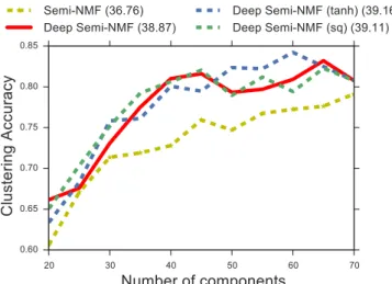
By using IGOs, the Deep Semi-NMF was able to out-perform the single-layer Semi-NMF as shown in Figures 9-10. Making use of these simple mixed-signed features improved the clustering accuracy considerably. It should be noted that in all cases, with the exception of the CMU PIE Pose experiment with IGOs, our Deep Semi-NMF outperformed all other methods with a difference in performance that is statistically significant (paired t-test,p0.01).
6.6 Supervised pre-training
As the optimization process of deep architectures is highly non-convex, the initialization point of the process is an important factor for obtaining good final represen-tation for the initial dataset. Following trends in deep learning [46], we show that supervised pretraining of our model on a auxiliary dataset and using the learned weights as initialization points for the unsupervised
20 30 40 50 60 70 Number of components 0.60 0.65 0.70 0.75 0.80 0.85 Clustering Accuracy Semi-NMF (36.76) Deep Semi-NMF (38.87)
Deep Semi-NMF (tanh) (39.16) Deep Semi-NMF (sq) (39.11)
Fig. 9. XM2VTS-IGO: Accuracy scores on clustering based on the representations learned by each model with respect to identities. The deep architectures are comprised of 2 hidden layers (2520-625-a) and the rep-resentations used were from the top layer. In parenthesis we show the AUC scores.
20 30 40 50 60 70 Number of components 0.65 0.70 0.75 0.80 Clustering Accuracy Semi-NMF (35.57) Deep Semi-NMF (37.16)
Deep Semi-NMF (tanh) (37.10) Deep Semi-NMF (sq) (36.13)
Fig. 10. CMU PIE-IGO: Accuracy scores on clustering based on the representations learned by each model with respect to identities. The deep architectures are comprised of 2 hidden layers (2048-625-a) and the rep-resentations used were from the top layer. In parenthesis we show the AUC scores.
Deep Semi-NMF algorithm can lead to significant per-formance improvements in regards to clustering accu-racy.
As an auxiliary dataset we use XM2VTS where we resize all the images to a 32x32 resolution to match the CMU PIE image resolution, which is our pri-mary dataset. Splitting the XM2VTS dataset to train-ing/validation sets, we learn weights Zxm2vts1,2 using a Deep WSF model with (625–a) layers, and regularization parameters λ={0,0.01}.
We then use the obtained weights Zxm2vts1,2 from the supervised task as an initialization point and perform unsupervised fine-tuning on the CMU PIE dataset. To
evaluate the resulting features, we once again perform clustering using thek-means algorithm.
In our experiments all the models with supervised pre-training outperformed the ones without, as shown
in Figure 11, in terms of clustering accuracy.
Addition-ally this validates our claim of how pretraining can be exploited to get better representations out of unlabelled data. 20 30 40 50 60 70 Number of components 0.4 0.5 0.6 0.7 0.8 Clustering Accuracy Multi-layer NMF (28.15) NMF (MUL) (25.75) NeNMF (28.45) Deep Semi-NMF (36.54) Semi-NMF (34.03) GNMF (29.18)
Deep Semi-NMF w/pretraining (38.10)
Fig. 11. Supervised pre-training: Clustering accuracy on the CMU PIE dataset, after supervised training on the XM2VTS dataset using a priori Deep Semi-NMF . In parenthesis we show the AUC scores.
6.7 Learning with Respect to Different Attributes
Finally, we conducted experiments for classification us-ing each of the three representations learned by our three-layered Deep WSF models when the input was the raw pixel intensities of our images of a larger subset of the CMU Multi-PIE dataset.
CMU Multi-PIE contains around 750,000 images of
337 subjects, captured under laboratory conditions in four different sessions. In this work, we used a subset of7,905images of 147subjects in 5 different poses and expressing 6 different emotions, which is the amount of samples that we had annotations and were imposed to the same illumination conditions. Using the annotations from [47], [48], we aligned these images based on a common frame. After that, we resized them to a smaller resolution of40×30. The database comes with labels for each of the attributes mentioned above: identity, illumi-nation, pose, expression. We only used CMU Multi-PIE for this experiment since we only had identity labels for our other datasets. We split this subset into a training and validation set of 2025 images, and the rest for testing. We compare the classification performance of an SVM classifier (with a penalty parameterγ= 1) using the data representations of the NMF, NMF, and Deep Semi-NMF models that have no attribute information. The
Model Pose Expression Identity Unsupervised Semi-NMF 99.73 81.50 36.46 NMF 100.00 80.68 49.12 Deep Semi-NMF 99.86 80.54 61.22 Semi CNMF 89.21 33.88 28.30 DNMF 100.00 82.22 55.78 Pr oposed WSF 100.00 81.50 63.81 WSF-MA 100.00 81.50 64.08 Deep WSF 100.00 82.90 65.17 TABLE 2
The performance in accuracy on the CMU Multi-PIE dataset using an SVM classifier on top of the features
learned. For the multi-layer models we used 3 layers corresponding to each of the attributes, and performed
classification using the features learned for the corresponding attribute. For the one-layer models, we
learned three different representations, one for each layer.
CNMF [24], DNMF [25], and our WSF models that have attribute labels only for the attribute we were classify-ing for, and our WSF-MA and Deep WSF that learned data representations based on all attribute information available. InTable 2, we demonstrate the performance in accuracy of each of the methods. In all of the methods, each feature layer has 100 components, and in the case of the Deep WSF model, we have used ∀i.λi= 10−3.
We also compared the performance of our Deep WSF with that of WSF and WSF-MA to see whether the different levels of representation amount to better performance in classification tasks for each of the at-tributes represented. In both cases, but also in compari-son with the rest state-of-the-art unsupervised and semi-supervised matrix factorization techniques, our pro-posed solution manages to extract better features for the task at hand as seen inTable 2for classification.
7
C
ONCLUSIONWe have introduced a novel deep architecture for semi-non-negative matrix factorization, the Deep Semi-NMF, that is able to automatically learn a hierarchy of at-tributes of a given dataset, as well as representations suited for clustering according to these attributes. Fur-thermore we have presented an algorithm for optimizing the factors of our Deep Semi-NMF, and we evaluate its performance compared to the single-layered Semi-NMF and other related work, on the problem of clustering faces with respect to their identities. We have shown
83.22 % 63.9 5% 100 % 79.7 3% 65.17 % 100% 100 % 79.9% 60.5 %
Fig. 12. A three layer Deep WSF model trained on CMU MultiPIE with only frontal illumination (camera 5). The bars depict the accuracy levels for the pose ( ), emotion ( ), and identity ( ) respectively, for each layer, with a linear SVM classifier.
that our technique is able to learn a high-level, final-layer representation for clustering with respect to the attribute with the lowest variability in the case of two popular datasets of face images, outperforming the considered range of typical powerful NMF-based techniques.
We further proposed Deep WSF, which incorporates knowledge from the known attributes of a dataset that might be available. Deep WSF can be used for datasets that have (partially) annotated attributes or even are a combination of different data sources with each one pro-viding different attribute information. We have demon-strated the abilities of this model on the CMU Multi-PIE dataset, where using additional information provided to us during training about the pose, emotion, and identity information of the subject we were able to uncover better features for each of the attributes, by having the model learning from all the available attributes simultaneously. Moreover, we have shown that Deep WSF could be used to pretrain models on auxiliary datasets, not only to speed up the learning process, but also uncover better representations for the attribute of interest.
Future avenues include experimenting with other ap-plications, e.g. in the area of speech recognition, espe-cially for multi-source speech recognition and we will investigate multilinear extensions of the proposed frame-work [49], [50].
A
CKNOWLEDGMENTSGeorge Trigeorgis is a recipient of the fellowship of the Department of Computing, Imperial College London, and this work was partially funded by it. The work of Konstantinos Bousmalis was funded partially from the Google Europe Fellowship in Social Signal Processing. The work of Stefanos Zafeiriou was partially funded by the EPSRC project EP/J017787/1 (4D-FAB). The work of Bj ¨orn W. Schuller was partially funded by the European
Community’s Horizon 2020 Framework Programme un-der grant agreement No. 645378 (ARIA-VALUSPA). The responsibility lies with the authors.
REFERENCES
[1] P. Paatero and U. Tapper, “Positive matrix factorization: A non-negative factor model with optimal utilization of error estimates of data values,”Environmetrics, vol. 5, no. 2, pp. 111–126, 1994. [2] J.-P. Brunet, P. Tamayo, T. R. Golub, and J. P. Mesirov, “Metagenes
and molecular pattern discovery using matrix factorization,” PNAS, vol. 101, no. 12, pp. 4164–4169, 2004.
[3] K. Devarajan, “Nonnegative matrix factorization: an analytical and interpretive tool in computational biology,” PLoS computa-tional biology, vol. 4, no. 7, p. e1000029, 2008.
[4] M. W. Berry and M. Browne, “Email surveillance using non-negative matrix factorization,”Computational & Mathematical Or-ganization Theory, vol. 11, no. 3, pp. 249–264, 2005.
[5] S. Zafeiriou, A. Tefas, I. Buciu, and I. Pitas, “Exploiting dis-criminant information in nonnegative matrix factorization with application to frontal face verification,”TNN, vol. 17, no. 3, pp. 683–695, 2006.
[6] I. Kotsia, S. Zafeiriou, and I. Pitas, “A novel discriminant non-negative matrix factorization algorithm with applications to facial image characterization problems.”TIFS, vol. 2, no. 3-2, pp. 588– 595, 2007.
[7] F. Weninger and B. Schuller, “Optimization and parallelization of monaural source separation algorithms in the openBliSSART toolkit,” Journal of Signal Processing Systems, vol. 69, no. 3, pp. 267–277, 2012.
[8] C. H. Ding, T. Li, and M. I. Jordan, “Convex and semi-nonnegative matrix factorizations,”IEEE TPAMI, vol. 32, no. 1, pp. 45–55, 2010. [9] C. Cing, X. He, and H. Simon, “On the equivalence of nonnegative matrix factorization and spectral clustering,” inProc. SIAM Data Mining, 2005.
[10] J. Herrero, A. Valencia, and J. Dopazo, “A hierarchical unsu-pervised growing neural network for clustering gene expression patterns.” Bioinformatics (Oxford, England), vol. 17, pp. 126–136, 2001.
[11] Y. Zhao and G. Karypis, “Hierarchical clustering algorithms for document datasets,”Data Mining and Knowledge Discovery, vol. 10, pp. 141–168, 2005.
[12] G. Tsoumakas and I. Katakis, “Multi-label classification: An overview,”International Journal of Data Warehousing and Mining, vol. 3, pp. 1–13, 2007.
[13] Y. Zhang and Z.-H. Zhou, “Multilabel dimensionality reduction via dependence maximization,” pp. 1–21, 2010.
[14] G. Trigeorgis, K. Bousmalis, S. Zafeiriou, and W. B. Schuller, “A Deep Semi-NMF Model for Learning Hidden Representations,” inICML, vol. 32, 2014.
[15] G. E. Hinton and R. R. Salakhutdinov, “Reducing the dimension-ality of data with neural networks,”Science, vol. 313, no. 5786, pp. 504–507, 2006.
[16] G. H. Golub and C. Reinsch, “Singular value decomposition and least squares solutions,”Numerische Mathematik, vol. 14, no. 5, pp. 403–420, 1970.
[17] S. Wold, K. Esbensen, and P. Geladi, “Principal component anal-ysis,”Chemometrics and intelligent laboratory systems, vol. 2, no. 1, pp. 37–52, 1987.
[18] D. D. Lee and H. S. Seung, “Algorithms for non-negative matrix factorization,” Advances in neural information processing systems, vol. 13, pp. 556–562, 2001.
[19] D. Cai, X. He, J. Han, and T. S. Huang, “Graph regularized nonnegative matrix factorization for data representation,”TPAMI, vol. 33, no. 8, pp. 1548–1560, 2011.
[20] J.-H. Ahn, S. Choi, and J.-H. Oh, “A multiplicative up-propagation algorithm,” inICML. ACM, 2004, p. 3.
[21] S. Lyu and X. Wang, “On algorithms for sparse multi-factor nmf,” inAdvances in Neural Information Processing Systems, 2013, pp. 602– 610.
[22] A. Cichocki and R. Zdunek, “Multilayer nonnegative matrix factorization,”Electronics Letters, vol. 42, pp. 947–948, 2006. [23] H. A. Song and S.-Y. Lee, “Hierarchical data representation model
- multi-layer nmf,”ICLR, vol. abs/1301.6316, 2013.
[24] H. Liu, Z. Wu, X. Li, D. Cai, and T. S. Huang, “Constrained Non-negative Matrix Factorization for Image Representation,”PAMI, vol. 34, pp. 1299–1311, 2012.
[25] I. Kotsia, S. Zafeiriou, and I. Pitas, “Novel discriminant non-negative matrix factorization algorithm with applications to facial image characterization problems,”TIFS, vol. 2, pp. 588–595, 2007. [26] M. Riesenhuber and T. Poggio, “Hierarchical models of object recognition in cortex.”Nature neuroscience, vol. 2, no. 11, pp. 1019– 1025, 1999.
[27] J. Malo, I. Epifanio, R. Navarro, and E. P. Simoncelli, “Nonlinear image representation for efficient perceptual coding,”TIP, vol. 15, pp. 68–80, 2006.
[28] K. Hornik, M. Stinchcombe, and H. White, “Multilayer feedfor-ward networks are universal approximators,” Neural networks, vol. 2, no. 5, pp. 359–366, 1989.
[29] Y. Nesterovet al., “Gradient methods for minimizing composite objective function,” 2007.
[30] D. M. Cvetkovic, M. Doob, and H. Sachs,Spectra of graphs: Theory and application. Academic press New York, 1980, vol. 413. [31] M. Belkin and P. Niyogi, “Using Manifold Structure for Partially
Labelled Classification,” inNIPS 2002, 2002, pp. 271–277. [32] M. Belkin, P. Niyogi, and V. Sindhwani, “Manifold regularization:
A geometric framework for learning from labeled and unlabeled examples,”JMLR, vol. 7, pp. 2399–2434, 2006.
[33] Y. Hao, C. Han, G. Shao, and T. Guo, “Generalized graph regu-larized non-negative matrix factorization for data representation,” inLecture Notes in Electrical Engineering, vol. 210 LNEE, 2013, pp. 1–12.
[34] M. Turk and A. Pentland, “Eigenfaces for Recognition,” 1991. [35] S. Li, X. W. H. X. W. Hou, H. J. Z. H. J. Zhang, and Q. S. C. Q. S.
Cheng, “Learning spatially localized, parts-based representation,” CVPR, vol. 1, 2001.
[36] T. Sim, S. Baker, and M. Bsat, “”the cmu pose, illumination, and expression database.”,” TPAMI, vol. 25, no. 12, pp. 1615–1618, 2003.
[37] K. Messer, J. Matas, J. Kittler, J. Luettin, and G. Maitre, “Xm2vtsdb: The extended m2vts database,” inInternational conference on audio and video-based biometric person authentication, vol. 964. Citeseer, 1999, pp. 965–966.
[38] N. Guan, D. Tao, Z. Luo, and B. Yuan, “NeNMF: an optimal gra-dient method for nonnegative matrix factorization,”TSP, vol. 60, no. 6, pp. 2882–2898, 2012.
[39] G. Tzimiropoulos, S. Zafeiriou, and M. Pantic, “Subspace learning from image gradient orientations,” 2012.
[40] C. Ding, T. Li, and M. I. Jordan, “Convex and semi-nonnegative matrix factorizations,”TPAMI, vol. 32, pp. 45–55, 2010.
[41] N. Gillis and A. Kumar, “Exact and Heuristic Algorithms for Semi-Nonnegative Matrix Factorization,” arXiv preprint arXiv:1410.7220, 2014.
[42] C. Boutsidis and E. Gallopoulos, “Svd based initialization: A head start for nonnegative matrix factorization,” Pattern Recognition, vol. 41, no. 4, pp. 1350–1362, 2008.
[43] M. Belkin and P. Niyogi, “Laplacian eigenmaps and spectral techniques for embedding and clustering.” inNIPS, vol. 14, 2001, pp. 585–591.
[44] W. Xu, X. Liu, and Y. Gong, “Document clustering based on non-negative matrix factorization,” inSIGIR. ACM, 2003, pp. 267–273. [45] Y. A. LeCun, L. Bottou, G. B. Orr, and K. R. M ¨uller, “Efficient backprop,” Lecture Notes in Computer Science (including subseries Lecture Notes in Artificial Intelligence and Lecture Notes in Bioinfor-matics), vol. 7700 LECTU, pp. 9–48, 2012.
[46] Y. Bengio, P. Lamblin, D. Popovici, and H. Larochelle, “Greedy layer-wise training of deep networks,”Advances in neural informa-tion processing systems, vol. 19, p. 153, 2007.
[47] C. Sagonas, G. Tzimiropoulos, S. Zafeiriou, and M. Pantic, “300 faces in-the-wild challenge: The first facial landmark Localization Challenge,” inCVPR, 2013, pp. 397–403.
[48] ——, “A semi-automatic methodology for facial landmark anno-tation,” inCVPR-W, 2013, pp. 896–903.
[49] S. Zafeiriou, “Discriminant nonnegative tensor factorization algo-rithms,”TNN, vol. 20, no. 2, pp. 217–235, 2009.
[50] ——, “Algorithms for nonnegative tensor factorization,” inTensors in Image Processing and Computer Vision. Springer, 2009, pp. 105– 124.
George Trigeorgisis pursuing a Ph.D. degree from Imperial College London.
Konstantinos Bousmalis is a researcher working with Google Robotics, California.
Stefanos Zafeiriou is a Lecturer in the Department of Computing, Imperial College London.
Bj ¨orn W. Schuller is a Lecturer in the Department of Computing, Imperial College London.