A Comparative Performance Analysis of TRMM 3B42 (TMPA) Versions 6 and 7 for
Hydrological Applications over Andean–Amazon River Basins
ZEDZULKAFLI,* WOUTERBUYTAERT,1CHRISTIANONOF,#BASTIANMANZ,#ELENATARNAVSKY,@ WALDOLAVADO,&ANDJEAN-LOUPGUYOT**
* Department of Civil and Environmental Engineering, Imperial College London, London, United Kingdom, and Universiti Putra Malaysia, Serdang, Malaysia
1Department of Civil and Environmental Engineering, and Grantham Institute for Climate Change, Imperial College
London, London, United Kingdom
#Department of Civil and Environmental Engineering, Imperial College London, London, United Kingdom @Department of Meteorology, University of Reading, Reading, United Kingdom
&Servicio Nacional de Meteorologı´a e Hidrologı´a, Lima, Peru
** Institut de Recherche pour le Developpement, Lima, Peru
(Manuscript received 22 May 2013, in final form 11 October 2013) ABSTRACT
The Tropical Rainfall Measuring Mission 3B42 precipitation estimates are widely used in tropical regions for hydrometeorological research. Recently, version 7 of the product was released. Major revisions to the algorithm involve the radar reflectivity–rainfall rate relationship, surface clutter detection over high terrain, a new reference database for the passive microwave algorithm, and a higher-quality gauge analysis product for monthly bias correction. To assess the impacts of the improved algorithm, the authors compare the version 7 and the older version 6 products with data from 263 rain gauges in and around the northern Peruvian Andes. The region covers humid tropical rain forest, tropical mountains, and arid-to-humid coastal plains. The authors find that the version 7 product has a significantly lower bias and an improved representation of the rainfall distribution. They further evaluated the performance of the version 6 and 7 products as forcing data for hydrological modeling by comparing the simulated and observed daily streamflow in nine nested Amazon River basins. The authors find that the improvement in the precipitation estimation algorithm translates to an increase in the model Nash–Sutcliffe efficiency and a reduction in the relative bias between the observed and simulated flows by 30%–95%.
1. Introduction
The Tropical Rainfall Measuring Mission (TRMM) produces global estimates of precipitation based on re-mote observations. The product of the 3B42 algorithm [hereafter referred to as the TRMM Multisatellite Pre-cipitation Analysis (TMPA)], which is high in spatial (0.258) and temporal (3 h) resolution, is a widely used forcing dataset for hydrometeorological applications such as hydrological modeling, especially in data-sparse re-gions (e.g.,Awadallah and Awadallah 2013;Li et al. 2012;
Khan et al. 2011;Wagner et al. 2009;Asante et al. 2008; Su et al. 2008).
There is consensus among studies using TMPA in and near tropical mountain regions (e.g., Ward et al. 2011; Scheel et al. 2011;Condom et al. 2011;Dinku et al. 2010; Nair et al. 2009;Bookhagen and Strecker 2008) about the limitation of the data, in particular, the poor quan-tification of high-precipitation events, which are the prev-alent form occurring in regions highly influenced by the intertropical convergence zone (ITCZ). As TMPA com-bines remote observations such as TRMM precipitation radar (TPR), passive microwave (PMW), and infrared (IR) from multiple low-Earth-orbiting and geostationary satellites and ground observations (Huffman et al. 2007), Denotes Open Access content.
Corresponding author address: Zed Zulkafli, Department of Civil and Environmental Engineering, Imperial College London, South Kensington Campus, London SW7 2AZ, United Kingdom. E-mail: [email protected]
This article is licensed under aCreative Commons Attribution 4.0 license.
DOI: 10.1175/JHM-D-13-094.1
various explanations for the estimation uncertainty are possible.
For example, the TMPA algorithm relies heavily on cloud-top (IR) temperatures from TRMM’s onboard in-struments, as well as from other participating geosta-tionary satellites in between TRMM satellite overpasses, as proxy measurements of rain [‘‘colder clouds pre-cipitate more’’ (Huffman et al. 2010, p. 10)]. It has been argued that in tropical mountain regions, the tempera-tures of orographic clouds well exceed the rain–no rain threshold imposed in the algorithm that can cause an un-derestimation of precipitation (Dinku et al. 2010). Indeed, estimates solely based on IR measurements, such as Pre-cipitation Estimation from Remote Sensing Information Using Artificial Neural Networks (PERSIANN; Hsu et al. 1997), have been found to underperform other satellite precipitation products in mountainous envi-ronments (Thiemig et al. 2012;Ward et al. 2011). Esti-mation using PMW observations has a stronger physical basis but remains problematic with warm rain clouds deficient in ice particles (Huffman et al. 2010; Dinku et al. 2010). The PMW sensor may also be insensitive at the scale of measurement, leaving very localized heavy rainfall cells undetected (Thiemig et al. 2012). Addi-tionally, TMPA’s poor estimation of extremes has been attributed to the optimization of the TPR’s reflectivity– rainfall rate (Z–R) relationship over moderate pre-cipitation rates, given their higher occurrence (Thiemig et al. 2012). Notwithstanding these limitations, it has also been shown with the TRMM 2A25 product (TPR-based estimates that feed into the 3B42 algorithm) that clear precipitation gradients can be observed over larger temporal scales over the Andes (Nesbitt and Anders 2009).
The TMPA version 6 algorithm is described in Huff-man et al. (2007), while changes in the version 7 algo-rithm at various processing levels are described in Huffman et al. (2010)andHuffman and Bolvin (2013) and are summarized here. They include the new Goddard profiling algorithm (GPROF) 2010 algorithm for PMW-based estimation that references TRMM’s available records of storm profiles, PMW brightness temperatures, and precipitation rates, replacing a reference database constructed using a cloud model in version 6. Addition-ally, the TMPA version 7 also incorporates more obser-vation datasets at different detection ranges than does version 6, notably, the 10-km resolution IR data to replace the Global Precipitation Climatology Centre (GPCC) histograms used in the early part of the time series (1997–2000) and the full time series of Micro-wave Humidity Sounder (MHS) and Special Sensor Microwave Imager/Sounder (SSM/IS) observations. A single-calibration reprocessed Advanced Microwave
Sounding Unit-B (AMSU-B) dataset from the National Oceanic and Atmospheric Administration (NOAA) satellite also replaces the prior version, for which two different calibration periods were used, thus removing some of the internal inconsistency present in TMPA version 6 (Huffman et al. 2007). Furthermore, the algorithm implements a final step gauge bias correction at the monthly scale, and while the GPCC monitoring product (version 2.0) and the NOAA Climate Prediction Cen-ter’s Climate Anomaly Monitoring System (CAMS) data product were previously used in the TMPA version 6 algorithm, the version 7 algorithm uses a new full data reanalysis (version 6.0) from GPCC that 1) interpolates anomalies instead of amounts and 2) incorporates a denser rain gauge network.
Over mountain regions, global and region-specific improvements were implemented in the TPR estima-tion, as detailed in a technical document (TRMM Pre-cipitation Radar Team 2011) and summarized here. In version 6, the algorithm was found to mistake the high level of surface clutter over the mountains for rain echo. It also mislocates surface echoes because of 1) inaccurate elevation data and 2) concealment by strong signals from heavy rainfall. The version 7 algorithm renews its elevation map for the Andes and Himalayas using data from the Shuttle Radar Topography Mission with 30-arc-s spacing (SRTM30) and introduces a repeat search al-gorithm for the surface echo that should improve its detection and thus the determination of clutter-free rain regions in the storm profile. This is expected to improve the quantification of light rain. Global changes such as theZ–Rrelationship based on a nonspherical rain drop distribution, an increase of 0.5 dB to stratiform pre-cipitation to compensate for heavy rain attenuation, and allowance for small convective storm cells favor higher estimations of heavy rainfall rates.
Few studies have looked into the performance of the TMPA version 7 precipitation product.Kirstetter et al. (2013), using data from TRMM 2A25 (TPR analysis) show that in the contiguous United States, bias against ground observations is reduced and correlation is im-proved. The same product provides an increase in total and convective rainfall over Asia south of 158S (Shiratsu et al. 2011). In a benchmarking exercise against radar observations in Japan,Nakagawa et al. (2011) saw no change in correlation but saw improved bias. Mean-while,Hobouchian et al. (2012)found increases in the probability of detection and equitable threat score as well as high extreme bias reduction from version 6 to version 7 of TMPA in South American regions south of 208S. These findings are encouraging for tropical moun-tain regions, where there is a growing body of modeling work using TMPA, but often with some level of
postprocessing required to improve the water balance (e.g.,Lavado-Casimiro et al. 2009;Arias-Hidalgo et al. 2013;Zulkafli et al. 2013). TMPA version 7 data will be increasingly used in modeling studies (e.g.,Espinoza et al. 2013), necessitating a full exploration of the implica-tions of the TMPA algorithm revisions on reducing data uncertainty. Therefore, the objective of this paper is to analyze if, how, and where TMPA version 7 is superior to version 6 in the Peruvian Andes region from a hydrolog-ical perspective. As the region covers some of the major climates and gradients found in the tropics, the findings will have a high potential for extrapolation to many other tropical regions relying on remote estimates of rainfall. 2. Methods and data
a. Study area
The study domain is located in north Peru and southeast Ecuador between 118S and 18N and between 808and 708W (Figs. 1a,b). The area covers humid trop-ical rain forest, troptrop-ical mountains, and arid-to-humid coastal plains.
The region’s climate has been discussed by various authors (Espinoza Villar et al. 2009;Garreaud et al. 2009; Casimiro et al. 2012; Buytaert et al. 2006; Kvist and Nebel 2001). The climate and seasonality (seeFig. 1c) is
controlled by large-scale meteorological phenomena such as the ITCZ and the South American monsoon system (SAMS;Marengo et al. 2012) that cause predominantly wet austral summers [December–February (DJF)]. In the austral winter [June–July (JJA)], the ITCZ band re-mains north of 58N but continues to cause some deep convection and rain in the northern parts of the Amazon basin (Espinoza Villar et al. 2009). Additionally, the Amazon regions experience large-scale stratiform pre-cipitation throughout much of the year from exposure to the humid tropical Atlantic easterly winds.
In the Pacific coast south of the Ecuador–Peruvian border, the von Humboldt oceanic current causes a cooler, drier climate regime throughout the year. The humid Pacific coast areas in Ecuador are less subject to this atmospheric cooling and experience a wetter sum-mer because of the predominance of the ITCZ (Fig. 1c). Over the Andes, the climate is complex and is primarily controlled by orography, windward/leeward effects, and the formation of local microclimates. The climate is wetter in the east slopes (Amazon) than it is in the west slopes because of the same climate drivers that affect the lowland regions.
In our analysis, we subdivided the area into six climate regions: Pacific coast, north and south; the Andes, west and east slopes; Amazon sub-Andes; and Amazon lowland FIG. 1. (a) Map of the study domain indicating the position of ground observation stations of various climate regions. The elevation of the Andes is in gray shading. The river basins are delineated based on the river network and the positions of streamflow monitoring stations, numbered corresponding toTable 2. (b) The map shows the geolocation of the study area. (c) The bar graph summarizes the precipitation regimes in each climate region. The values plotted are the mean monthly climatology averaged over each region’s rain gauges.
(summarized in Table 1). We define the Andes as the regions above 1500 m, and the Amazon sub-Andes as the eastern Andean slopes located at altitudes of 13006 200 m, which is a belt of high orographic precipitation (above 3500 mm yr21) illustrated in a previous study of Andean transects byBookhagen and Strecker (2008).
b. Precipitation data
TMPA version 6 and 7 for the time domain 1998–2009 were obtained from the NASA archive (ftp://disc2.nascom. nasa.gov/ftp/data/s4pa//TRMM_L3/) and aggregated to daily, monthly, seasonal, and annual values. Out of 1920 pixels (0.258 30.258) in the study domain, 144 are collo-cated with the ground observation stations. The number of collocated pairs are tabulated inTable 1.
Historical rain records (years 1998–2009) were ob-tained from the national weather station networks of Peru (Servicio Nacional de Meteorologıa e Hidrologıa) and Ecuador (Instituto Nacional de Meteorologıa e Hidrologıa). The records consist of daily time series from 184 gauges in Peru and monthly time series from 79 gauges in Ecuador.
c. Precipitation analysis
The intercomparison was performed in terms of 1) the mean annual rainfall (mm yr21), 2) the mean annual relative bias [Eq. (1)], and 3) the mean seasonal bias [mm day21; Eq. (2)] at each ground observation loca-tion. For each region, we also averaged the time series of all paired observations and inspected the bias at the monthly scale: REL.BIAS5
å
T t51 PTMPA,t2PGAUGE,tå
T t51 PGAUGE,t 3100% (1) and BIAS5å
T t51 PTMPA,t2PGAUGE,t. (2)We further analyzed TMPA’s skill at estimating var-ious precipitation event types by comparing their dis-tributions of daily rainfall rates to those recorded by the rain gauges. In presenting our results, we adopted the following precipitation classification criteria (mm day21): zero rain, 0–0.2; light rain, 0.2–1.0; moderate rain, 1.0–5.0, heavy rain, 5.0–15, very heavy rain, 15–50, and extremely heavy rain, above 50. We computed the probability of occurrence of each precipitation type from the entire time series for each satellite–gauge pair. For each region and precipitation class, the statistics are summarized in a boxplot to represent all data pairs, and the probability distributions are compared between the rain gauge, TMPA version 6, and TMPA version 7 datasets.
d. Hydrological analysis
To gauge the impact on hydrological performance, the water balance was evaluated at multiple nested hydro-logical basins tributary to the Amazon river by calcu-lating the long-term average runoff ratio [RR; Eq.(3)] using both versions of the precipitation product. The corresponding evapotranspiration (ET) estimation is also compared to values from the literature and poten-tial evapotranspiration (PET) values from Moderate Resolution Imaging Spectroradiometer (MODIS; values from a representative year, 2001, were used):
RR5
å
T t51 QRIVERGAUGE,tå
T t51 PTMPA,t . (3)Additionally, both TMPA versions were evaluated in terms of the output of a hydrological model constructed for the basins. Detailed model development has been TABLE1. The criteria used to define various regions for the analysis. The variablenis the number of satellite–gauge observation pairs located in each region. Climate regimes are given in terms of seasons DJF, March–May (MAM), JJA, and September–November (SON).
No. Subregion
Elevation
(m) Climate driver Climate regime n
1 Pacific coast, north 0–1500 ITCZ Humid DJF and MAM;
dry JJA and SON
19 2 Pacific coast, south 0–1500 von Humboldt current, ITCZ Humid DJF and MAM;
dry JJA and SON
20
3 Andes west slope .1500 Mountain terrain, ITCZ Humid DJF and MAM;
dry JJA and SON
85 4 Andes east slope .1500 Mountain terrain, ITCZ, orography Weak seasonality, drier JJA 61 5 Amazon sub-Andes 1100–1500 Orography, ITCZ, SAMS, tropical
Atlantic winds
Weak seasonality, drier JJA 8 6 Amazon lowland 0–1200 ITCZ, SAMS, tropical Atlantic winds Weak seasonality, drier JJA 70
described in previous work (Zulkafli et al. 2013). Briefly, we used a land surface model called the Joint UK Land Environment Simulator (JULES; Best et al. 2011) to generate hydrological fluxes over 0.1258 30.1258grids. JULES requires near-surface meteorological data as input, which it uses to solve fully coupled energy, water, and carbon balance equations, producing a continuous output of ET and runoff (surface and subsurface). This runoff is then fed into a delay function routing model to produce streamflows that are compared to observations. Daily streamflow data were provided by the Geo-dynamical, hydrological and biogeochemical control of erosion/alteration and material transport in the Amazon basin (HYBAM) project from nine stations in Ecuador and Peru (Table 2). Information from global and local maps is used to describe the land surface properties, and the simulations (1998–2008) were performed with few perturbations to the original model parameters. The performance scores such as Nash–Sutcliffe efficiency (NSE) and the relative bias between the simulated runoff and the observed daily streamflows were tabu-lated and compared between the TMPA versions. 3. Results and discussion
a. Mean annual, seasonal, and monthly bias
Figures 2a–cshow the mean and the relative change of the mean annual precipitation in TMPA versions 6 and 7. A clear spatial trend is observed—there is a sub-stantial increase in the total precipitation amounts from version 6 to version 7 along the Andes and the Pacific coast in the north that results in corresponding re-ductions in the negative bias against rain gauge obser-vations (Figs. 2d,e). Figure 2f shows that, with the exception of a few gauge locations in the Pacific coast in
Peru, the direction of change in the relative bias is pos-itive. This observation agrees with an increase in gauge densities in these areas between the different datasets used in versions 6 and 7 and suggests a large role in the bias correction within the algorithm. In spite of this, TMPA version 7 continues to overall underestimate pre-cipitation, except in the northern Andean regions down to the Ecuador–Peruvian border, where it is now over-estimating compared to the rain gauges.
A seasonal analysis demonstrated the main reduction of the negative bias from version 6 to version 7 occurring along the Andean range and in the coastal region in Ecuador during the wet season (DJF and MAM) (Fig. 3). TMPA version 7 also tends to cause some overestimations over the Andes (west and east slopes) in the north, and these overestimations persist during the drier seasons (JJA and SON). Changes between versions 6 and 7 over the lowland Amazon and the Amazon sub-Andes re-gions are relatively small with no apparent seasonal trend, which may be explained by the low seasonality in their climate. Altogether, there is evidence of an increase in wet season deep convective heavy precipitation amounts and an increase (to the point of overestimation) of the dry season light rain, and this is further confirmed in the time series analysis of the monthly bias between TMPA and gauge estimates.
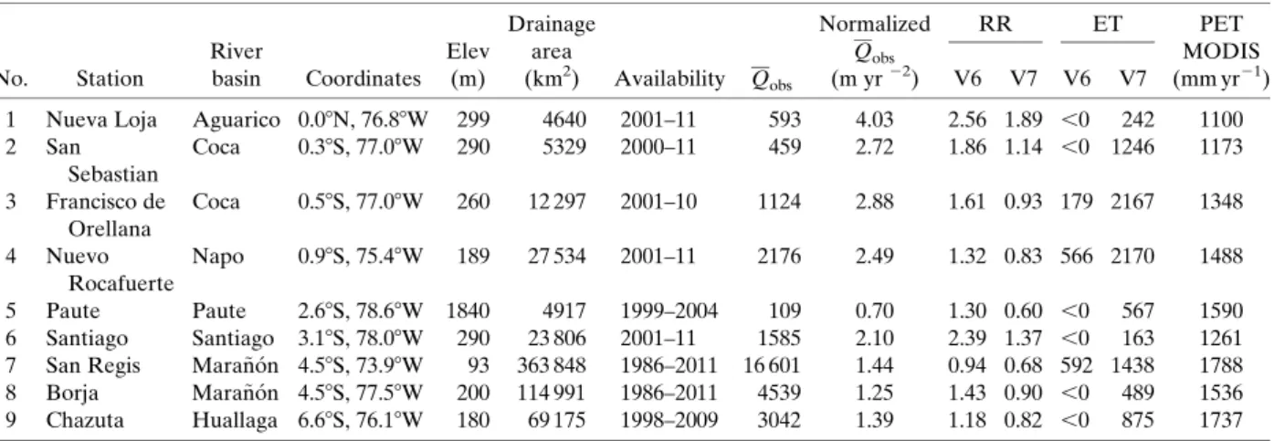
Figure 4shows that TMPA versions 6 and 7 monthly biases against gauge data are highly correlated and that the direction of change is positive throughout most of the time series. As the biases in version 6 tend to be neg-ative, this resulted in biases shifting toward zero in ver-sion 7, and in some cases, such as the Pacific lowland in the south, toward positive biases. A strong seasonality in the negative bias reduction (highest in DJF) is observed in the coastal regions (north and south) and the west TABLE2. Streamflow stations and water balance summary. The numbers refer toFig. 1. The mean observed dischargeQobs(m3s21) is calculated using all available data. Runoff ratio is given for version 6 (RR V6) and 7 (RR V7) and the corresponding evapotranspiration (mm yr21) is calculated from the water balance equation assuming zero long-term change in storage for version 6 (ET V6) and 7 (ET V7).
No. Station River basin Coordinates Elev (m) Drainage area (km2) Availability Qobs Normalized Qobs (m yr22) RR ET PET MODIS (mm yr21) V6 V7 V6 V7
1 Nueva Loja Aguarico 0.08N, 76.88W 299 4640 2001–11 593 4.03 2.56 1.89 ,0 242 1100 2 San Sebastian Coca 0.38S, 77.08W 290 5329 2000–11 459 2.72 1.86 1.14 ,0 1246 1173 3 Francisco de Orellana Coca 0.58S, 77.08W 260 12 297 2001–10 1124 2.88 1.61 0.93 179 2167 1348 4 Nuevo Rocafuerte Napo 0.98S, 75.48W 189 27 534 2001–11 2176 2.49 1.32 0.83 566 2170 1488 5 Paute Paute 2.68S, 78.68W 1840 4917 1999–2004 109 0.70 1.30 0.60 ,0 567 1590 6 Santiago Santiago 3.18S, 78.08W 290 23 806 2001–11 1585 2.10 2.39 1.37 ,0 163 1261 7 San Regis Mara~non 4.58S, 73.98W 93 363 848 1986–2011 16 601 1.44 0.94 0.68 592 1438 1788 8 Borja Mara~non 4.58S, 77.58W 200 114 991 1986–2011 4539 1.25 1.43 0.90 ,0 489 1536 9 Chazuta Huallaga 6.68S, 76.18W 180 69 175 1998–2009 3042 1.39 1.18 0.82 ,0 875 1737
Andes, which are the regions with the strongest sea-sonalities. A few exceptions are the prominent positive biases with version 7 in the sub-Andes between 2002 and 2006, and in the Pacific lowlands in the south, during the same time period and in 2007. These are drier summer periods associated with El Nino episodes of drought, as~ these regions experience increased dry air subsidence from intensified convection over the Pacific Ocean.
b. Precipitation rates distribution
Figures 5a–eprovide further insight into the shifts in the daily rainfall distributions estimated in versions 6 and 7. In version 6, the TMPA distributions are more strongly skewed toward light-to-moderate intensity pre-cipitation compared to the gauge distributions across all regions. This observation concurs with the reported un-derestimation of extreme high precipitation by TMPA version 6 in the literature. The version 7 product effectively shows a shift in the distribution toward higher-intensity
precipitation and an increase in the internal variability across the range of precipitation rates. Consequently, there is a reduction in the bias between TMPA and rain gauge distributions over the Andes and sub-Andes, particu-larly for heavy and very heavy precipitation, where the medians of the distributions align closer than previously. The underestimation, nevertheless, persists to some ex-tent, and light-to-moderate rain continues to be over-estimated most severely in the west slopes of the Andes. We recognize that TMPA’s underestimation of high extremes may simply be a reflection of the nature of their data as a spatial average when compared to point rain gauge data. However, TMPA also shows an over-estimation of zero-rain days, whereas, by their nature, spatial averages should observe lower no-rain days compared to point estimates. This may be caused by the low sampling frequency and consequently missed short-duration precipitation events between satellite mea-surements. The overestimation of dry days is considerably FIG. 2. The spatial variability of the (a),(b) mean annual precipitation; (d),(e) mean relative bias against ground observation; and (c),(f) changes between TMPA versions 6 and 7. Country borders are outlined in gray. River basins are outlined in black in (a)–(c). The elevation of the Andes is in gray shading in (d)–(f).
reduced in version 7 and may have to do with the re-finement to the surface reflectivities routine in the TPR algorithm that improves the determination of rain sig-nals from clutter, and as well as the recalibration of the TPR’sZ–Rrelationship toward a general increase in the precipitation rates.
c. Impact on the water balance and hydrological simulation
The impact of the TMPA algorithm change to the water balance in several hydrological basins tributary to the Amazon basin (Fig. 2) are presented in terms of runoff ratios (Table 2). TMPA version 6 typically gen-erates physically unrealistic runoff ratios above 1, highlighting the consistent regional underestimation of precipitation. Version 7 generates substantially reduced runoff ratios, with values closer to those expected for humid tropical basins, even in the small Andean basin of Paute. Some unrealistically high runoff ratios remain in basins with a high areal runoff, such as Santiago, San Sebastian, and Nueva Loja located in southeastern
Ecuador, which reflect the prevailing underestimation of heavy rain in version 7 TMPA, as discussed insection 3b. The increase in precipitation amounts also results in ET estimates closer to MODIS-based estimates averaged for each basin (Table 2, last column) and literature values of ET (600, 1200, and 1300 mm yr21median values for the Andes and tropical montane and lowland rain forests, re-spectively; see Zulkafli et al. 2013, and references therein). The improvement in the water balance translates di-rectly into hydrological modeling performance, as seen in Fig. 6 and Table 3. Simulations driven by TMPA version 7 produce a closer estimate of daily streamflows to the observed time series and result in an increase in the modeling efficiency (NSE score) in all nine basins. At San Regis, which is the largest basin analyzed, the relative bias between simulated and observed flows de-creased from237.8% to22.0%, which is a reduction of 95%. Here, the averaged precipitation bias reduction from 235% to 210% parallels the reduction in the simulated discharge. In Chazuta, where there is a good coverage of rain gauges across the basin, we performed FIG. 3. The spatial variability of the seasonal biases (mm day21) between TMPA versions 6 and 7 and ground observations. The elevation
an additional simulation using rain gauge data interpolated with kriging to serve as a benchmark and found it to underperform (NSE of 20.19, bias of 230.0%) the simulation forced by TMPA version 7 (NSE of 0.43, bias of218.7%). This implies a high potential skill of TMPA version 7 in ungauged catchments, a sentiment echoed byXue et al. (2013)based on their hydrological evalu-ation of TMPA version 7 against version 6 and ground observations in Bhutan.
Improvements at varying degrees were observed elsewhere, most notably in the humid north Andean
basins of Paute, Nuevo Rocafuerte, and Francesco de Orellana, which suggests the role of an improved high precipitation estimation. Nevertheless, the hydrographs also show that the variations in the peaks are still poorly modeled, except in the larger basins. This reflects the continued underestimation of extremes by TMPA, as well as the limitations of the hydrological model in representing surface runoff generation processes in mountain environments. In spite of this, our work has demonstrated that the forcing uncertainty is significantly reduced in TMPA version 7. This enables further work FIG. 4. The average monthly bias in TMPA versions 6 and 7 vs gauge by climate region.
to focus on developing more accurate process repre-sentations for the tropical Andes.
4. Conclusions
The TMPA versions 6 and 7 intercomparison work completed over six climate regions in the tropical Andes–Amazon showed an overall increase in pre-cipitation, especially in the Pacific lowlands (north) and the Andes. Our results corroborate the findings of the few existing validation studies on TMPA version 7 that show better agreement with gauge data compared to version 6. Our closer inspection of the bias distributions indicated that the primary improvement is in the re-duction of the negative bias of the wet season’s high extreme. We could infer that the positive outcome is attributable to a combination of the changes in the al-gorithm that improves heavier rain quantification, and we hypothesize that 1) a higher number of rain gauges used during bias correction, 2) the TPR radar recali-bration toward higher precipitation rates, and 3) an improved GPROF 2010 algorithm for the PMW-based precipitation estimates play a large role. The hydrolog-ical performance of TMPA with version 7 increased considerably over nine hydrological basins in the region, increasing our confidence in the use of TMPA as forcing data for modeling applications to complement ground
observations in tropical mountain regions where they are usually scarce or inaccessible. This applies not only to hydrological studies but also to other modeling ap-plications that benefit from the use of precipitation as driving data.
We recognize several pathways for further evaluation. First, by analyzing a composite, final product, we restrict our ability to directly attribute the improvements to TMPA version 7 to the different steps of the TMPA al-gorithm. The logical next step is therefore to evaluate multiple precipitation products from the various levels of the TMPA processing individually, which will enable us to identify and inform the main contributors to the overall uncertainty. For example, one could compare the TMPA’s research product to the real-time product and quantify the added value of a regional gauge correction of the satellite product. Second, from a water resources standpoint where the main interest is in the means and extremes, it is sensible to look at TMPA’s representation of entire distributions of precipitation rates compared to those of gauge data, as we have presented in our analysis. However, for operational applications such as forecasting, early warning, or risk analysis, further performance in-dices, such as false alarm ratios, missed volumes, and the probability of detection, should be considered. In this context, a direct pixel-to-point satellite–gauge comparison will have to accommodate the fundamental challenge of FIG. 5. (a)–(e) Precipitation rate distributions in TMPA version 6 vs 7, gauge, and TMPA vs gauge, according to precipitation types. The precipitation type is characterized based on precipitation intensities (mm day21): zero rain, 0–0.2; light rain, 0.2–1.0; moderate rain, 1.0– 5.0; heavy rain, 5.0–15; very heavy rain, 15–50; and extremely heavy rain, above 50. The boxplots in each interval represent the variability between the data points, which are probability of occurrence for each pixel-to-point pair. The boxes extend from the first to the third quartiles of the data points, and the whiskers extend to the highest value within 1.5 times the interquartile range. The dots represent values outside this range.
resolving the mismatch in the temporal and spatial support of the data products in both occurrence and amounts, that is, the timing of the precipitation event versus that of a satellite retrieval and the spatial in-tegration of satellite estimates that smooths extremes. Aggregating point rain gauge data to the satellite pixel using a simple averaging or more complex geostatistical interpolation methods, or conversely, downscaling sat-ellite data to finer-resolution estimates using geo-physical predictors such as elevation [as has been shown in Fang et al. (2013)], should be implemented before a reasonable point-to-pixel comparison can be made.
Finally, conclusions from our analysis of a set of data from a specific region and the potential for extrapolation should ideally be further corroborated using cross vali-dation with rain gauge data from other regions. This extended analysis can also explore the data performance at different spatial and temporal scales.
Acknowledgments.This research is funded by the U.K.
NERC Grant NE/I004017/1 and the Ministry of Higher Education, Malaysia. We thank Jhan-Carlo Espinoza Villar and two anonymous reviewers for constructive comments.
REFERENCES
Arias-Hidalgo, M., B. Bhattacharya, A. E. Mynett, and A. van Griensven, 2013: Experiences in using the TMPA-3B42R satellite data to complement rain gauge measurements in the Ecuadorian coastal foothills. Hydrol. Earth Syst. Sci., 17, 2905–2915, doi:10.5194/hess-17-2905-2013.
Asante, K. O., G. A. Arlan, S. Pervez, and J. Rowland, 2008: A linear geospatial streamflow modeling system for data sparse environments. Int. J. River Basin Manage., 6, 233–241, doi:10.1080/15715124.2008.9635351.
Awadallah, A., and N. Awadallah, 2013: A novel approach for the joint use of rainfall monthly and daily ground station data with TRMM data to generate IDF estimates in a poorly gauged arid region. Open J. Mod. Hydrol., 3, 1–7, doi:10.4236/ ojmh.2013.31001.
Best, M. J., and Coauthors, 2011: The Joint UK Land Environment Simulator (JULES), model description—Part 1: Energy and water fluxes.Geosci. Model Dev., 4, 677–699, doi:10.5194/ gmd-4-677-2011.
Bookhagen, B., and M. Strecker, 2008: Orographic barriers, high-resolution TRMM rainfall, and relief variations along the eastern Andes.Geophys. Res. Lett.,35,L06403, doi:10.1029/ 2007GL032011.
Buytaert, W., R. Celleri, P. Willems, B. De Bievre, and G. Wyseure, 2006: Spatial and temporal rainfall variability in mountainous areas: A case study from the south Ecuadorian Andes.J. Hy-drol.,329,413–421, doi:10.1016/j.jhydrol.2006.02.031.
Casimiro, W. S. L., J. Ronchail, D. Labat, J. C. Espinoza, and J.-L. Guyot, 2012: Basin-scale analysis of rainfall and runoff in Peru (1969–2004): Pacific, Titicaca and Amazonas drainages. Hy-drol. Sci. J.,57,625–642, doi:10.1080/02626667.2012.672985. Condom, T., P. Rau, and J. C. Espinoza, 2011: Correction of
TRMM 3B43 monthly precipitation data over the mountain-ous areas of Peru during the period 1998–2007.Hydrol. Pro-cesses,25,1924–1933, doi:10.1002/hyp.7949.
Dinku, T., S. Connor, and P. Ceccato, 2010: Comparison of CMORPH and TRMM-3B42 over mountainous regions of Africa and South America.Satellite Rainfall Applications for Surface Hydrology,M. Gebremichael and F. Hossain, Eds., Springer, 193–204.
Espinoza, J. C., J. Ronchail, F. Frappart, W. Lavado, W. Santini, and J. L. Guyot, 2013: The major floods in the Amazonas River and tributaries (western Amazon basin) during the 1970–2012 period: A focus on the 2012 flood.J. Hydrometeor,
14,1000–1008, doi:10.1175/JHM-D-12-0100.1.
Espinoza Villar, J. C., and Coauthors, 2009: Spatio-temporal rainfall variability in the Amazon basin countries (Brazil, Peru, Bolivia, Colombia, and Ecuador). Int. J. Climatol., 29, 1574–1594, doi:10.1002/joc.1791.
Fang, J., J. Du, W. Xu, P. Shi, M. Li, and X. Ming, 2013: Spatial downscaling of TRMM precipitation data based on the oro-graphical effect and meteorological conditions in a moun-tainous area. Adv. Water Resour., 61, 42–50, doi:10.1016/ j.advwatres.2013.08.011.
Garreaud, R. D., M. Vuille, R. Compagnucci, and J. Marengo, 2009: Present-day South American climate. Palaeogeogr. Palaeoclimatol. Palaeoecol., 281, 180–195, doi:10.1016/ j.palaeo.2007.10.032.
Hobouchian, M., P. Salio, D. Vila, and Y. Skabar, 2012: Validation of satellite precipitation estimates over South America with a network of high spatial resolution observations.Sixth Int. Precipitation Working Group,S~ao Jose dos Campos, Brazil, IPWG. [Available online atwww.isac.cnr.it/;ipwg/meetings/ saojose-2012/training/Hobouchian.pdf.]
Hsu, K., X. Gao, S. Sorooshian, and H. V. Gupta, 1997: Pre-cipitation estimation from remotely sensed information using artificial neural networks. J. Appl. Meteor., 36,1176–1190, doi:10.1175/1520-0450(1997)036,1176:PEFRSI.2.0.CO;2. Huffman, G. J., and D. T. Bolvin, 2013: TRMM and other
data precipitation data set documentation. Global Change Master Directory, NASA, 40 pp. [Available online at
ftp://precip.gsfc.nasa.gov/pub/trmmdocs/3B42_3B43_doc. pdf.]
——, and Coauthors, 2007: The TRMM Multi-satellite Pre-cipitation Analysis: Quasi-global, multi-year, combined-sensor precipitation estimates at fine scale.J. Hydrometeor.,8, 38–55, doi:10.1175/JHM560.1.
——, R. Adler, D. Bolvin, and E. Nelkin, 2010: The TRMM Multi-Satellite Precipitation Analysis (TMPA). Satellite Rainfall Applications for Surface Hydrology,M. Gebremichael and F. Hossain, Eds., Springer, 3–22.
Khan, S. I., and Coauthors, 2011: Hydroclimatology of Lake Vic-toria region using hydrologic model and satellite remote sensing data.Hydrol. Earth Syst. Sci.,15,107–117, doi:10.5194/ hess-15-107-2011.
Kirstetter, P.-E., Y. Hong, J. J. Gourley, M. Schwaller, W. Petersen, and J. Zhang, 2013: Comparison of TRMM 2A25 products version 6 and version 7 with NOAA/NSSL ground radar-based national mosaic QPE.J. Hydrometeor.,14,661–669, doi:10.1175/JHM-D-12-030.1.
TABLE3. The model NSE [calculated for version 6 (NSE V6) and 7 (NSE V7)] and relative bias [calculated for version 6 (QV6 and
PV6) and 7 (QV7 andPV7)] compared between simulations using TMPA versions 6 and 7. The variablemindicates the number of gauges located inside each basin used to calculate the relative bias in precipitation.
No. Hydrological station NSE V6 NSE V7
Relative bias (%) m QV6 QV7 PV6 PV7 1 Nueva Loja 22.13 21.60 277.1 269.4 20.16 0.31 2 2 San Sebastian 24.08 21.39 272.1 239.1 20.78 20.51 1 3 Francisco de Orellana 22.44 20.47 260.3 216.5 — — 0 4 Nuevo Rocafuerte 22.45 20.22 252.5 29.5 20.78 20.51 1 5 Paute 20.92 0.06 290.0 230.7 20.39 0.10 6 6 Santiago 22.06 20.89 285.5 260.2 20.47 20.05 10 7 San Regis 21.23 0.53 237.8 22.0 20.35 20.11 108 8 Borja 21.53 20.34 273.3 240.4 20.39 20.11 56 9 Chazuta 20.55 0.43 252.4 218.7 20.27 20.10 35
Kvist, L., and G. Nebel, 2001: A review of Peruvian flood plain forests: Ecosystems, inhabitants and resource use.For. Ecol. Manage.,150,3–26, doi:10.1016/S0378-1127(00)00679-4. Lavado-Casimiro, W., D. Labat, J. L. Guyot, J. Ronchail, and
J. J. Ordonez, 2009: TRMM rainfall data estimation over the Peruvian Amazon–Andes basin and its assimilation into a monthly water balance model.IAHS Publ.,333,245–252. Li, X.-H., Q. Zhang, and C.-Y. Xu, 2012: Suitability of the TRMM
satellite rainfalls in driving a distributed hydrological model for water balance computations in Xinjiang catchment, Poyang lake basin.J. Hydrol.,426–427,28–38, doi:10.1016/ j.jhydrol.2012.01.013.
Marengo, J. A., and Coauthors, 2012: Recent developments on the South American monsoon system.Int. J. Climatol.,32,1–21, doi:10.1002/joc.2254.
Nair, S., G. Srinivasan, and R. Nemani, 2009: Evaluation of multi-satellite TRMM derived rainfall estimates over a western state of India.J. Meteor. Soc. Japan,87,927–939, doi:10.2151/jmsj.87.927. Nakagawa, K., N. Yoshida, and T. Higashiuwatoko, 2011: PR V7 2A25 evaluation using the conventional radar in Japan. TRMM Doc., JAXA, 11 pp. [Available online athttp://www. eorc.jaxa.jp/TRMM/documents/PR_algorithm_product_ information/doc_pr_v7/A01_PRV7_WS_20110603_NICT_ Nakagawa_EN.pdf.]
Nesbitt, S., and A. Anders, 2009: Very high resolution precipitation climatologies from the Tropical Rainfall Measuring Mission precipitation radar.Geophys. Res. Lett.,36,L15815, doi:10.1029/ 2009GL038026.
Scheel, M. L. M., M. Rohrer, Ch. Huggel, D. Santos Villar, E. Silvestre, and G. J. Huffman, 2011: Evaluation of TRMM Multi-satellite Precipitation Analysis (TMPA) performance in the Central Andes region and its dependency on spatial and temporal resolution.Hydrol. Earth Syst. Sci.,15,2649–2663, doi:10.5194/hess-15-2649-2011.
Shiratsu, F., F. A. Furuzawa, and K. Nakamura, 2011: The com-parison of precipitation statistics between TRMM-PR 2A25 V6 and V7.TRMM/PR Product Version 7 Workshop,
Nagoya University, Nagoya, Japan. [Available online at
http://www.eorc.jaxa.jp/TRMM/documents/PR_algorithm_ product_information/doc_pr_v7/A06_v7_WS_20110603_ shiratsu.pdf.]
Su, F., Y. Hong, and D. Lettenmaier, 2008: Evaluation of TRMM multisatellite precipitation analysis (TMPA) and its utility in hydrologic prediction in the La Plata basin.J. Hydrometeor.,9, 622–640, doi:10.1175/2007JHM944.1.
Thiemig, V., R. Rojas, M. Zambrano-Bigiarini, V. Levizzani, and A. De Roo, 2012: Validation of satellite-based precipitation products over sparsely gauged African river basins.J. Hy-drometeor.,13,1760–1783, doi:10.1175/JHM-D-12-032.1. TRMM Precipitation Radar Team, 2011: Tropical rainfall
mea-suring mission (TRMM) precipitation radar algorithm: In-struction manual for version 7. Tech. Rep., JAXA/NASA, 170 pp. [Available online athttp://www.eorc.jaxa.jp/TRMM/ documents/PR_algorithm_product_information/pr_manual/ PR_Instruction_Manual_V7_L1.pdf.]
Wagner, S., H. Kunstmann, A. Bardossy, C. Conrad, and R. R. Colditz, 2009: Water balance estimation of a poorly gauged catchment in West Africa using dynamically down-scaled meteorological fields and remote sensing infor-mation. Phys. Chem. Earth, 34, 225–235, doi:10.1016/ j.pce.2008.04.002.
Ward, E., W. Buytaert, L. Peaver, and H. Wheater, 2011: Evalua-tion of precipitaEvalua-tion products over complex mountainous terrain: A water resources perspective.Adv. Water Resour.,
34,1222–1231, doi:10.1016/j.advwatres.2011.05.007.
Xue, X., Y. Hong, A. S. Limaye, J. J. Gourley, G. J. Huffman, S. I. Khan, C. Dorji, and S. Chen, 2013: Statistical and hy-drological evaluation of TRMM-based Multi-Satellite Pre-cipitation Analysis over the Wangchu basin of Bhutan: Are the latest satellite precipitation products 3B42V7 ready for use in ungauged basins? J. Hydrol., 499, 91–99, doi:10.1016/ j.jhydrol.2013.06.042.
Zulkafli, Z., W. Buytaert, C. Onof, W. Lavado, and J. L. Guyot, 2013: A critical assessment of the JULES land surface model hydrology for humid tropical environments. Hydrol. Earth Syst. Sci.,17,1113–1132, doi:10.5194/hess-17-1113-2013.