Procedia Computer Science 17 ( 2013 ) 1047 – 1054
1877-0509 © 2013 The Authors. Published by Elsevier B.V.
Selection and peer-review under responsibility of the organizers of the 2013 International Conference on Information Technology and Quantitative Management
doi: 10.1016/j.procs.2013.05.133
Information Technology and Quantitative Management (ITQM2013)
An Embedded Backward Feature Selection Method for MCLP
Classification Algorithm
Meihong Zhu
*, Jie Song
School of Statistics, Capital University of Economics and Business, Zhang Jia Lu Kou 121, Fengtai District, Beijing, 100070, China
*Corresponding author.
E-mail address: [email protected]
Abstract
Feature selection is very crucial for improving classification performance, especially in the case of high-dimensional data classification.Different classification algorithms tend to select different optimal feature subsets. Based on detailed analysis of the characteristics of Multiple Criteria Linear Programming (MCLP) classification algorithm, a feature selection criterion is presented and an embedded backward feature selectionprocedure is designed for MCLP in this paper. Experiments on four datasets (artificial and real-world) are carried out, and the effectiveness of the presented method is assessed. Results show that it achieves good performance as expected.
© 2013 The Authors. Published by Elsevier B.V.
Selection and/or peer-review under responsibility of the organizers of the 2013 International Conference on Computational Science
Keywords: Multiple Criteria Linear Programming, Feature Selection, Embedded, Backward
_______________________________________________________________________________________________________________________________________
1.Introduction
In the domain of classification, feature or variable selection (hereinafter referred to as FS) is very crucial for improving classification performance, especially in the case of high-dimensional data classification. By eliminating irrelative and redundant features, FS is conducive to improve learning speed, predictive accuracy and simplicity and comprehensibility of learned results [1, 2]. Although many feature selection methods have been presented, none of them can be suitable for all classification algorithms. Theoretical and experimental researches show that, different classification algorithms tend to select different optimal feature subsets. So, for a specific classification algorithm, we need to analyze its characteristics and find the corresponding FS methods © 2013 The Authors. Published by Elsevier B.V.
Selection and peer-review under responsibility of the organizers of the 2013 International Conference on Information Technology and Quantitative Management
Open access under CC BY-NC-ND license.
for it. This paper intends to design an effective FS method for Multiple Criteria Linear Programming (MCLP) classification algorithm. It is organized as follows: Section 2 reviews some widely used FS methods. Section 3 describes the principle, model and properties of MCLP. In section 4, an embedded backward FS method for MCLP is proposed. In section 5, the effectiveness of this method is verified on four datasets. Finally, the availability of it is analyzed and concluded.
2.Feature selection
FS techniques are generally divided into three categories, depending on whether and how they combine the FS process with the learning algorithm: filter methods, wrapper methods and embedded methods [3-5].
When a FS method is used as a data preprocessing technique, it is often separated from the specific learning task or algorithm, and it is usually called a filter method. In a filter method, the goodness of a feature/feature subset is dependent on some general measure, such as distance measure, information measure, dependence measure, consistency measure or accuracy measures [4]. With this filter method, all features are ranked according to one or some of above measures, and only the highest ranking features are selected. The result of FS also relies on general characteristics of training data, but it does not involve any learning algorithm. A filter method also provides a very easy way to calculate and can simply scale to large-scale datasets since it only has a short computing time. However, the selected features may be not useful for a specific classification algorithm.
A wrapper method embeds a feature selection process within a classification algorithm. In a wrapper method, a search is conducted in the feature space, evaluating the goodness of each found feature subset by the estimation of the accuracy of the specific classifier to be used, training the classifier only with the found features. Because a wrapper method incorporates the interaction between feature selection and classification model, it is claimed that a wrapper method can get better predictive accuracy estimate than a filter method [2]. However, its computational cost is higher than a filter method and often it has a higher risk of over-fitting.
Compared with filter and wrapper, in an embedded method, the feature search process is embedded into the classification algorithm, and the learning process and the feature selection process can t be separated. Similar to a wrapper method, an embedded method includes the interaction with the classifier, while at the same time, it can save computation cost largely than a wrapper method.
3.MCLP classification algorithm
MCLP classification model was proposed by Shi [6, 7] based on optimization theory. A two-class MCLP classification model can be depicted as follows:
Here we have a training set T which includes n cases, r input features and a two-class target (output) feature labeled by Ai = (Ai1 , Air) represent the ith case, where i = 1, . . . , n. MCLP aims at finding the best coefficient vector of r features X = (x1 , xr )T, and a boundary value b, to correctly classify each existing case into Bad or Good; that is,
i i i i
A X b, A Bad and A X b, A Good.
Due to incomplete linear separability of two classes in real-world datasets, some cases will be misclassified. Two kinds of distance are defined to measure the degree of misclassification or correct classification of thecase Ai :
If Ai is misclassified, let ibe the distance between Aiand boundary b; If Ai is correctly classified, let i be the distance between Ai and boundary b.
The objective of MCLP is minimizing and maximizing simultaneously. The initial MCLP classification model M1 is
Where Aiis given; Xand b are unrestricted; and i, i .
Since there exists conflict between the above two objectives, a compromise solution approach is introduced to balance them [6], and thus, this multi-objective linear programming model M1 can be transformed into a single-objective model.
- i i be i i be > 0). Then four kinds of
regret are defined to measure the difference between actual values and ideal values of the above two objectives. Detailedly, If - i i > , the regret is defined as d + = i i ; otherwise, d + = 0. If - i i < , the regret is defined as d- = *
i i; otherwise, d - =0. Thus, the following three formulae always hold: (i) i i = d
-- d+, (ii) |
i i | = d- + d+, and (iii) d - , d+ e also always hold:
(i) - i i = d- - d +, (ii) | - i i| = d- + d+, and (iii) d - , d+ 0. The above four regrets are hoped to be as little as possible. So M1 can be changed into a single-objective linear programming model M2.
Where Ai, *, and * are given, X and b are unrestricted, and i , i , d -, d+ , d - , d+ In practice, * can be given as 0.00001, * as 99999, and b as 1.
In the MCLP classification model, the idea of linear programming is applied to determine a hyperplane for separating classes. The objective reflects its controlling on classification error, and classification discriminant criteria are included in the constraints. If X is solved, a labelled or unlabeled case Ai can be classified by the
value of AiX: Ai is AiX<b; Ai AiX>b.
Compared with other classification algorithms, MCLP is simple and direct, free of any assumptions, flexible in defining and modifying parameters, and high on classification accuracy. It has been widely used in business fields, such as credit card analysis, fraud detection, and so on.
4.An embedded backward feature selection method for MCLP
Supposing the best coefficient vector of all features X = (x1, . . . , xr )T has been obtained by implementing MCLPon the training set T. Applying the solution X on T, the corresponding optimal classification accuracy can be estimated. Now dimension reduction will be investigated in the premise of keeping the present optimal result.
From the model M2, It can be seen that, the effect mechanism of afeature Fj on classification result is that, it directly affects the constraints (3) and (4), and then affects the constraints (1) and (2), and finally the objective Z. For a case Ai, the effect of Fj on Z is AijXj. In the constraints (3) and (4), the effects of Fj onthem can be
4 3 2 1 M Z Good i A , i i b X i A Bad i A , i i b X i A d d i d d i : to Subject d d d d Minimize i i 2 Good A , b X A Bad A , b X A : to Subjiect ) ( Maximize and Minimize i i i i i i i i 1 i i i i M
demonstrated in the Table 1.
Table 1. The effect mechanism of Fj on the constraints (3) and (4)
n1, and that n2. Based on the training result of the last time, m1 cases are misclassified while n1 - m1 cases are correctly classified in c
m2 cases are misclassified while n2 m2
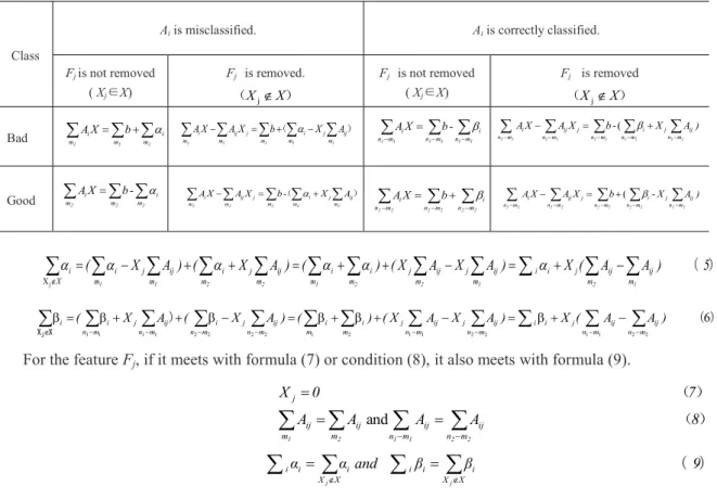
of Fj on terms i i and i i can be demonstrated in the Table 2 and the formulae (5) and (6).
Table 2. The integrated effect of Fjon and i i
For the feature Fj, if it meets with formula (7) or condition (8), it also meets with formula (9).
Class
Aiis misclassified. Ai is correctly classified.
Fj is not removed. ( Xj X) Fj is removed. X Xj Fj is not Removed. ( Xj X) Fj is removed. X Xj Bad AiX b i AiX-AijXj b ( i AijXj) AiX b- i AiX-AijXj b-( i AijXj) Good AiX b- i AiX-AijXj b-( i AijXj) AiX b i AiX-AijXj b ( i-AijXj) Class
Ai is misclassified. Ai is correctly classified.
Fj is not removed ( Xj X) Fj is removed. X Xj Fj is not removed ( Xj X) Fj is removed X Xj Bad Good 6 1 1 2 2 1 1 2 2 2 1 2 2 2 2 1 1 1 1 n m n m ij ij j i i m n n m ij j ij j m i m i m n ij j m n i m n ij j m n i i ( X A ( X A ) ( ) (X A X A ) X ( A A ) ; ; ;M 8 A A A A 7 0 X 1 1 2 2 1 2 n m n m ij ij m m ij ij j and 9 and X X i i i X X i i i j j j X 5 ) A A ( X ) A X A X ( ) ( ) A X ( ) A X ( 2 1 2 1 2 1 2 2 1 1 m m ij ij j i i m ij jm ij j m i m i m ij j m i m ij j m i X i 2 2 2 2 2 m ij j m m i jm ij m i A X b X A X A -1 1 1 m i m m iX b A 1 1 1 1 1 m ij j m i m m ij j m i A X b X A X A 1 1 1 1 1 1 n m i m n m n iX b A - AX AX b X A) 1 1 1 1 1 1 1 1 1 1 nm ij j m n i m n m n nm j ij i -( 2 2 2 m i m m i b X A -2 2 2 2 2 2 n m i m n m n iX b A AX AX b X A) 2 2 2 2 2 2 2 2 2 2 n m ij j m n i m n m n n m j ij i ( -i i
This means that removing Fj does not change the constraints (1) and (2) and thus the objective Z. According to this idea, feature Fj meeting with (7) or (8) can be eliminated on the next round of training. In practice there are few features which can exactly meet with (7) or (8). So only features approximately according with (7) or (8) can be found. It is hoped that formulae (10) and (11) are all as little as possible.
Here formula (10) indicates the effect of Fj on , and formula (11) on . Considering the inconsistency between (10) and (11) in ranking features, they can be synthesized into one item. Because of the same importance between i iand i i in objective Z (10) and (11) should be the same important.
Then, the feature elimination/selection criterion is designed as formula (12).
According to the training results of the last
fe values can be removed in the next training round.
From the former item of formula (12 j reflects the separability of feature Fj on the two object classes. If the former item of formula (12) is large, it means Fj is an important feature for classification.
Compared with some other FS j reflects the effect of feature Fj on separating
of the two object classes by considering misclassified cases and correctly classified cases respectively. Xj measures the sensitivity of the output with respect to Fj. If |Xj | is small, then removing Fj does not produce large effect on the output. From the angle of feature selection process, this method is a backward FS method. According to feature search strategy, it applies a heuristic search strategy. Because the FS procedure is embedded into the classification process, it can be viewed as an embedded FS method.
5.Experimental arrangement and analysis
5.1.Data for analysis
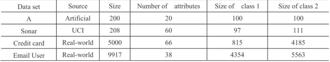
Here four datasets are used to appraise the effect of the proposed FS method. The characteristics of them are described in the Table 3. In the dataset A, the first three features, F1, F2 and F3, are purposely designed and all cases distributed in the space of the first three features as shown in the Figure 1. Another two features F4 and F5 are designed as F4=2F1 and F5=F2+F3. Other 15 features are simply random variables whose values are between 0 and 1. According to general viewpoint, F4 and F5 are redundant features, and F6-F20 are all irrelative features. In the Sonar dataset, there are high correlations between two adjacent features and low correlations among other features. In the Credit Card and the Email User datasets, only low correlations exist among features.
Table 3. The characteristics of four datasets
Data set Source Size Number of attributes Size of class 1 Size of class 2
A Artificial 200 20 100 100
Sonar UCI 208 60 97 111
Credit card Real-world 5000 66 815 4185
Email User Real-world 9917 38 4354 5563
12 A A A A j m n n m ij ij m m ij ij 1 1 2 2 1 2 | X | | -| | -| j 11 X A A 10 X ) A A 1 1 2 2 1 2 m n n m j ij ij m m j ij ij | -| | -( | i i i i
Fig. 1. The distribution of cases in the three-dimensional space of F1,F2 and F3
5.2.Feature selection procedure for MCLP
Considering computing cost, the two large datasets--the Credit Card and the Email User, are randomly divided into training sets and test sets respectively. In the Credit Card dataset, 800(400+400) cases are used as training datum and the rest as test datum. In the Email User dataset, 2000(1000+1000) cases are used as training datum and the rest as test datum. FS procedures are implemented on the training sets and the final model evaluations are executed on the tests. Because of the randomness in partitioning of dataset into training set and test set, five rounds of partitioning are implemented on the Credit Card and the Email User respectively. The detailed operation is presented in Figure 2 by taking the example of the Credit Card dataset.
_______________________________________________________________________________________ For l=1 to 5
Step1. Partition the Credit Card into training set TRl and test set Tel randomly.
--- TRl1=TRl (The initial training set of lth partition is set as TRL.)
For p=1 to sl (Loop of FS Process in lth partitioning ) Step2. Run MCLP on TRlp, and solution Xlp is generated.
Step3. Compute AiXlp for Aiin TRlp, and decide whether Aiis correctly classified.
Step3. Put m1lp n1lp-m1lp
m2lp n2lp-m2lp
Step4. Compute for each feature Fj respectively.
jlp for each Fj respectively.
Step6. Rank all values.
the whole accuracy on TRlp. If they begin to degrade obviously, end the loop of p, go to step 10. Otherwise, go to step 8.
Step8. Remove the feature F* with the smallest Step 9.TRlP=TRlp- F*
p=p+1 end of p.
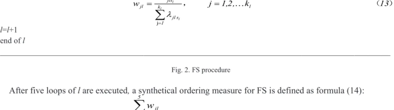
--- Step10. Supposing the loop of p is ended in the slth interation, then kl (=66-sl) features are left in TRL finally, and ranking weight for each of the kl features is computed as formula (13):
lp 1 lp 1 2lp 2lp lp 1 2lp n m n m ij ij m m ij ij A A A A and
l=l+1
end of l
_______________________________________________________________________________________ Fig. 2. FS procedure
After five loops of l are executed, a synthetical ordering measure for FS is defined as formula (14):
The selected kl features among five different partitions maybe are different, so k is not smaller than kl. According to formula (14), k features are ranked and 30 (<k) features with larger Wj are selected in the end.
On the five original training sets-TR1 ,TR2 TR3 TR4 and TR5, the above 30 features are selected respectively, and five new classifiers C1,C2,C3,C4 and C5 are trained. Applying them on the corresponding test sets TE1, TE2,
TE3, TE4 and TE5, five partitions of test accuracy are computed and their average is used as the accuracy estimation of FS .It can be noted that, there exits very weak correlations among input features in the Credit Card dataset, so several features with sma taneously removed in step 8.
As for the Email User, only 15 features are selected finally from it.
For the two small datasets, A and Sonar, FS procedures are directly executed on them and the effects of feature selection are also measured on them. Because of the strong correlation among features, eliminating a feature will bring remarkable change of ranking of other features. So in each step of feature selection, only one 5.3.Experimental results and analysis
According to experimental results on the four datasets, three aspects of important conclusions for MCLP are abstracted.
Firstly, MCLP has some similar characteristics to some other classification algorithms with respect to FS. When two input features are highly correlative, one of them is judged as redundant and is eliminated. In the artificial dataset A, F4 is perfectly correlated with F1. So F4 is eliminated at the first interaction of training. Similarly, F2 is highly correlated with F3, and F5 is the linear combination of F2 and F3. Then one of the three features, F2, is redundant and is removed in the first interaction, too. Features with prominent difference (especially, mean) between two different classes are thought as important features for classification. If there exist correlations among features at some degree, removing one feature will bring change of ranking of other features. Under this circumstance, features only can be eliminated one by one while removing features in bulk at one step is unreasonable.
However different to general conclusions, some random generated features with almost equal means between different classes are still selected into the final feature subset. For example, in the artificial dataset A, F6-F20 are all random generated features with almost equal means between two different classes, but some of them are still left in the training set in the end.
Finally the FS criterion
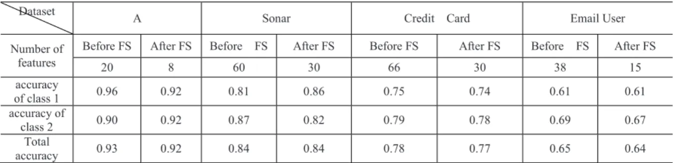
in the end is significantly smaller than that of the original feature set. Modeling on the smaller feature subset, computational efficiency is improved while classification accuracy does not obviously degrade. The experimental results on the four datasets are shown in the Table 4.
13 k , 2 , 1 j w k l 1 jls jls jl l l l j 14 ) k k ( k , , 2 , 1 j 5 w w l 5 1 l jl j
Table 4. The experimental results on the four datasets
6.Conclusions
In this paper, an embedded backward FS method is specially designed for MCLP classification algorithm. Similar to some filter methods, the j reflects the importance of feature Fj on classifying the two object classes by considering misclassified cases and correctly classified cases respectively. At the same time, j includes the coefficient Xj of Fj which represents the sensitivity of the output with respect to Fj. Experiments on one artificial dataset and three real-world datasets have been carried out. Results show that it achieves good performance and it is effective for MCLP. However, comparison of it with other popular feature selection criteria is not implemented and its advantage or disadvantage is not investigated in this paper.
Acknowledgement
This research has been financially supported by the Talent Improvement Plan of Beijing Education Committee --the Innovation Team Plan of Measurement and Research on Consumer s Confidence. It also has partially supported by a grant of National Natural Science Foundation of China (No. 11201316).
References
[1]A. Blum and P. Langley. Selection of Relevant Features and Examples in Machine Learning. Artificial Intelligence, 97:245-271, 1997.
[2] R. Kohavi and G. John. Wrappers for Feature Subset Selection. Artificial Intelligence, 97(1-2):273-324, 1997.
[3] I. Guyon and A. Elisseeff. An Introduction to Variable and Feature Selection. Journal of Machine Learning Research, vol. 3: 1157-1182, 2003.
[4] G.Victo Sudha George and Dr. V.Cyril Raj. Review on Feature Selection Techniques and the Impact of SVM for Cancer Classification Using Gene Expression Profile. International Journal of Computer Science & Engineering Survey (IJCSES) Vol.2, No.3, August 2011.
[5] C.Lazar, J.Taminau J, S. Meganck and et.al.. A survey on filter techniques for feature selection in gene expression microarray analysis. IEEE/ACM Trans Comput Biol Bioinform. 2012 Jul-Aug; 9(4):1106-19. [6]Y. Shi and P. L. Yu. Goal Setting and Compromise Solutions. B. Karpak and S. Zionts editors , Multiple Criteria Decision Making and Risk Analysis Using Microcomputers. Berlin: Springer 1989. 165 203.
[7] Y.Shi, Y. Peng and et.al.. Data mining via Multiple Criteria Linear Programming: Applications in Credit Card Portfolio Management. Information Technology and Decision Making 2002,1 1 : 145-166.
[8] UCI Irvine Machine Learning Repository, available online: http://archive.ics. uci.edu/ml/.
Dataset A Sonar Credit Card Email User
Number of features
Before FS After FS Before FS After FS Before FS After FS Before FS After FS
20 8 60 30 66 30 38 15 accuracy of class 1 0.96 0.92 0.81 0.86 0.75 0.74 0.61 0.61 accuracy of class 2 0.90 0.92 0.87 0.82 0.79 0.78 0.69 0.67 Total accuracy 0.93 0.92 0.84 0.84 0.78 0.77 0.65 0.64