Learning to skip state updates in recurrent neural networks

(1)

Universitat Polit`

ecnica de Catalunya

Escola T`

ecnica Superior d’Enginyeria de Telecomunicaci´

o de Barcelona

Learning to Skip State Updates

in Recurrent Neural Networks

V´ıctor Campos Cam´

u˜

nez

Advisors:

Xavier Gir´

o-i-Nieto, Jordi Torres, Brendan Jou, Shih-Fu Chang

A thesis submitted in fulfillment of the requirements for the degree of the

Master in Telecommunications Engineering

(2)

(3)

Abstract

Recurrent Neural Networks (RNNs) continue to show outstanding performance in sequence modeling tasks. However, training RNNs on long sequences often face challenges like slow infer-ence, vanishing gradients and difficulty in capturing long term dependencies. In backpropagation through time settings, these issues are tightly coupled with the large, sequential computational graph resulting from unfolding the RNN in time. We introduce the Skip RNN model which extends existing RNN models by learning to skip state updates and shortens the effective size of the computational graph. This network can be encouraged to perform fewer state updates through a novel loss term. We evaluate the proposed model on various tasks and show how it can reduce the number of required RNN updates while preserving, and sometimes even improving, the performance of the baseline models.

Keywords: machine learning, deep learning, recurrent neural networks, sequence modeling, conditional computation.

(4)

Resum

Les Xarxes Neuronals Recurrents (de l’anglès, RNNs) mostren un alt rendiment en tasques de modelat de seqüències. Tot i aix´ı, entrenar RNNs en seqüències llargues sol provocar dificultats com una inferència lenta, gradients que s’esvaeixen i dificultats per capturar depèndencies tem-porals a llarg terme. En escenaris ambbackpropagation through time, aquests problemes estan estretament relacionats amb la longitud i la seqüencialitat del graf computacional resultant de desdoblar la RNN en el temps. Presentem Skip RNN, model que extén arquitectures recurrents existents, permetent-les aprendre quan ometre actualitzacions del seu estat i escur¸cant aix´ı la longitud efectiva del graf computacional. Aquesta xarxa pot ser estimulada per efectuar menys actualitzacions d’estat a través d’un nou terme a la funció de cost. Evaluem el model proposat en una sèrie de tasques i demostrem com pot reduir el nombre d’actualitzacions de la RNN mentre preserva, o fins i tot millora, el rendiment dels models de referència.

Paraules clau: aprenentatge automàtic, aprenentatge profund, xarxes neuronals recurrents, modelat de seqüències, computació condicional.

(5)

Resumen

Las Redes Neuronales Recurrentes (del inglés, RNNs) muestran un alto rendimiento en tareas de modelado de secuencias. Aún as´ı, entrenar RNNs en secuencias largas suele provocar difi-cultades como una inferencia lenta, gradientes que se desvanecen y difidifi-cultades para capturar dependencias temporales a largo plazo. En escenarios con backpropagation through time, estos problemas están estrechamente relacionados con la longitud y la secuencialidad del grafo com-putacional resultante de desdoblar la RNN en el tiempo. Presentamos Skip RNN, un modelo que extiende arquitecturas recurrentes existentes, permitiéndoles aprender cuándo omitir actualiza-ciones de su estado y acortando as´ı la longitud efectiva del grafo computacional. Esta red puede ser estimulada para efectuar menos actualizaciones de estado a través de un nuevo elemento en la función de coste. Evaluamos el modelo propuesto en una serie de tareas y demostramos cómo puede reducir el número de actualizaciones de la RNN mientras preserva, o incluso mejora, el rendimiento de los modelos de referencia.

Palabras clave: aprendizaje autom´atico, aprendizaje profundo, redes neuronales recurrentes, modelado de secuencias, computaci´on condicional.

(6)

Acknowledgements

In the first place, I would like to thank my advisors: Shih-Fu, Brendan, Jordi and Xavi. This thesis would not have been possible without them. Thanks Shih-Fu for inviting me to develop this project in your lab at Columbia University, a experience I really enjoyed; Brendan, for your help and advice since my very first steps in deep learning research; Jordi, for giving me the opportunity to join BSC and the great years to come. Xavi, your devotion deserves a special mention. I am very grateful for it and the countless opportunities you always find for your students, making Barcelona a better place for deep learning research every single day.

This project would not have been possible without friends and colleagues at the Barcelona Supercomputing Center. Thanks M´ıriam for keeping our office chats even with an ocean between us. I am very grateful to the support team for their help and making the research process easier and faster.

The last six months in New York have been one of the best experiences in my life. There are many people who made it so enjoyable, probably too many to be listed here. Some goodbyes were extremely hard, but I am certain that we will see each other again. See you soon.

This thesis is the final chapter in a six year adventure at ETSETB. There have been many obstacles along the road, which would have been impossible to overcome without friends who were there every day transforming problems into laughter. Romero, Chema, Fullana, Jim´enez, Ferran: we may not go to class together anymore, but who knows what we maystart up someday...

Y por último, pero no menos importante, este trabajo va dedicado a mi familia. Por vuestro sacrificio para darme la oportunidad y la estabilidad para dedicarme a lo que me apasiona sin tener que preocuparme de nada más. Por el apoyo incondicional tanto en los buenos como los malos momentos a lo largo de los años. Por estar cerca aún estando a más de 6.000km de distancia. Muchas gracias.

(7)

Revision history and approval record

Revision Date Purpose

0 15/07/2017 Document creation

1 15/08/2017 Document revision

2 17/08/2017 Document approval

DOCUMENT DISTRIBUTION LIST

Name e-mail

V´ıctor Campos [email protected]

Xavier Gir´o-i-Nieto [email protected]

Jordi Torres [email protected]

Brendan Jou [email protected]

Shih-Fu Chang [email protected]

Written by: Reviewed and approved by: Reviewed and approved by:

Date 15/07/2017 Date 17/08/2017 Date 17/08/2017

Name V´ıctor Campos Name Xavier Gir´

o-i-Nieto Name Shih-Fu Chang

Position Project Author Position Project

Supervi-sor Position

Project Supervisor

(8)

List of Figures

4.1 Model architecture of the proposed Skip RNN. (a) Complete Skip RNN archi-tecture, where the computation graph at time step t is conditioned on ut. (b) Architecture when the state is updated, i.e. ut = 1. (c) Architecture when the update step is skipped and the previous state is copied, i.e. ut= 0. (d)In prac-tice, redundant computation is avoided by propagating ∆˜ut between time steps when ut= 0. . . 11

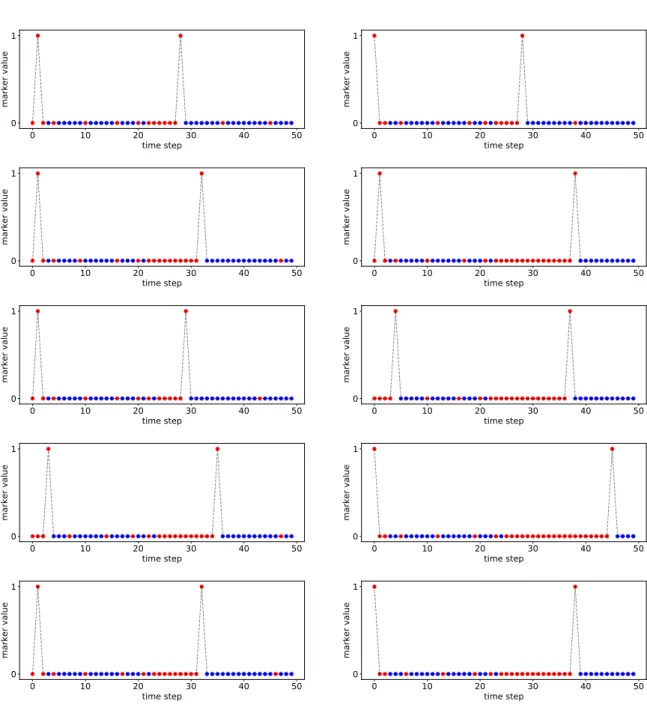
5.1 Sample usage examples for the Skip GRU withλ= 10−5 _{on the adding task. Red} dots indicate used samples, whereas blue ones are skipped. . . 15 5.2 Accuracy evolution during training on the validation set of MNIST. The Skip GRU

exhibits lower variance and faster convergence than the baseline GRU. A similar behavior is observed for LSTM and Skip LSTM, but omitted for clarity. Shading shows maximum and minimum over 4 runs, while dark lines indicate the mean. . 17 5.3 Sample usage examples for the Skip LSTM with λ = 10−4 _{on the test set of}

MNIST (top), MNIST-17 (middle) and MNIST-56 (bottom). Red pixels are used, whereas blue ones are skipped. . . 17 5.4 Accuracy evolution during the first 300 training epochs on the validation set of

UCF-101 (split 1). Skip LSTM models converge much faster than the baseline LSTM. . . 19

A.1 Sample usage examples for the Skip GRU withλ= 10−5 _{on the adding task. Red} dots indicate used samples, whereas blue ones are skipped. . . 28 A.2 Sample usage examples for the Skip LSTM with λ = 10−4 _{on the frequency}

discrimination task with Ts = 0.5ms. Red dots indicate used samples, whereas blue ones are skipped. The network learns that using the first samples is enough to classify the frequency of the sine waves, in contrast to a uniform downsampling that may result in aliasing. . . 29

(11)

List of Tables

3.1 Hyperparameters defining the jumping behavior of LSTM-Jump. . . 8

5.1 Results for the adding task, displayed asmean_±stdover four different runs. The task is considered to be solved if the MSE is at least two orders of magnitude below the variance of the output distribution. . . 14 5.2 Results for the frequency discrimination task, displayed as mean_±std over four

different runs. The task is considered to be solved if the classification accuracy is over 99%. Models with the same cost per sample (λ > 0) converge to a similar number of used samples under different sampling conditions. . . 15 5.3 Accuracy and used samples on the test set of MNIST after 600 epochs of training.

Results are displayed asmean±stdover four different runs. . . 16 5.4 Accuracy and used samples on the test set of IMDB for different sequence lengths.

Results are displayed asmean_±stdover four different runs. . . 18 5.5 Accuracy and used samples on the validation set of UCF-101 (split 1). . . 19

6.1 Cost of the project. Other equipment includes campus services, office supplies and hardware, e.g. the employed laptop and auxiliary monitor. . . 20

(12)

List of Abbreviations

NN NeuralNetwork

RNN Recurrent NeuralNetwork LSTM Long Short-TermMemory GRU GatedRecurrent Unit GPU GraphicsProcessingUnit

(13)

Chapter 1

Introduction

1.1

Motivation

Methods based on deep neural networks have established the state-of-the-art in computer vision tasks [32, 53, 23], machine translation [56], speech generation [43] and even defeated the world champion in the game of Go [50]. Although the development of these algorithms spans over many decades [35], their potential has been unlocked by the increased computational power of specific accelerators, e.g. Graphical Processing Units (GPUs), and the creation of large-scale datasets [15, 28]. Those readers who are not familiar with deep learning techniques may prefer to read Chapter 2, which gives an overview of the most basic concepts related to neural networks, before diving deeper in the contents of this thesis.

Recurrent Neural Networks (RNNs) have become the standard approach for practitioners when addressing machine learning tasks involving sequential data. Besides the increase in computa-tional power and publicly available data, improved architectures and training algorithms have been key for the success of RNNs. Gated units, such as the Long Short-Term Memory [25] (LSTM) and the Gated Recurrent Unit [10] (GRU), were designed to deal with the vanishing gradients problem commonly found in RNNs [8] that precluded their application during years. These architectures have popularized thanks to their impressive results in a variety of tasks such as machine translation [5], language modeling [61] or speech recognition [20].

RNNs process data sequentially in order to capture temporal dependencies. This inherently sequential behavior results in challenging training and deployment, especially when dealing with long sequences. These challenges include throughput degradation, slower convergence during training and memory leakage, even for gated architectures [41]. Sequence shortening techniques, which can be seen as a sort of conditional computation [7, 6, 14] in time, can alleviate these issues. The most common approaches, such as cropping discrete signals or reducing the sampling rate in continuous signals, are heuristics and can be suboptimal. In contrast, we propose a model that is able to learn which samples (i.e. elements in the input sequence) need to be used in order to solve the target task. Consider a video understanding task as an example: scenes with large motion may benefit from high frame rates, whereas only a few frames are needed to capture the semantics of a mostly static scene.

(14)

which samples in a sequence need to be used in order to solve the task at hand. Such subsampling mechanism needs to be integrated in the RNN itself, as opposed to a pre-processing step, and needs to be data-driven instead of being in heuristics. Moreover, the sample selection process has to be dynamic, i.e. each input sequence may be subsampled in a different way depending on their actual content. Our contributions include:

• A novel modification for existing RNN architectures that allows them to skip state updates, decreasing the number of inherently sequential operations to be performed, without requir-ing any additional supervision signal. This model, called Skip RNN, adaptively determines whether the state needs to be updated or it can be copied to the next time step, thus skipping computation. It can be seamlessly introduced into existing architectures to reduce the number of required RNN updates while preserving, and sometimes even improving, the performance of the baseline models.

• We show how the network can be encouraged to perform fewer state updates by adding a new penalization term during training, allowing to easily train models targeting different computational budgets.

• The proposed modification is implemented on top of well known RNN architectures, namely LSTM and GRU, and the resulting models show promising results in a series of sequence modeling tasks. In particular, the proposed Skip RNN architecture is evaluated on (1) the adding task, (2) sine wave frequency discrimination, (3) digit classification, (4) sentiment analysis in movie reviews, and (5) action classification in video.

This thesis is structured as follows. A brief introduction to deep learning is given in Chapter 2, which may come in handy for readers who are not familiar with the field. Chapter 3 provides an overview of the related work and techniques that bear some similarity with the proposed solution. The Skip RNN model is described in Chapter 4 and evaluated in a series of tasks in Chapter 5. Chapter 6 gives an estimation of the costs associated to the development of the project. Discussion and future research directions are provided in Chapter 7. Finally, appendices include additional qualitative results for the experiments and the pre-print uploaded to arXiv1.

1.2

Hardware and Software Resources

This project was developed using the resources provided by the Barcelona Supercomputing Center. In particular, the MinoTauro2 cluster was been used. The cluster has 39 nodes equipped with two NVIDIA K80 dual-GPUs each, resulting in up to four concurrent processes running in parallel in each node. Having access to several nodes at the same time proved itself crucial for tuning hyperparameters and performing different runs for each experiment. Evaluating the proposed models on such a broad set of tasks would have been unfeasible without access to these computing resources.

Experiments were implemented with TensorFlow3, using CUDA and cuDNN for fast GPU primitives. This framework was chosen due to previous experience and the fact that it was already available in the MinoTauro cluster. Code is publicly available athttps://github.com/ imatge-upc/skiprnn-2017-tfm/. 1 https://arxiv.org/ 2_{https://www.bsc.es/innovation-and-services/supercomputers-and-facilities/minotauro/} 3 https://www.tensorflow.org/

(15)

1.3

Work Plan

Being this a research-oriented project, it was difficult to define a detailed work plan ahead of time: the next steps to take were generally conditioned on the latest obtained results. Besides, since the field of deep learning is extremely active, new results are published and uploaded to arXiv every day and may affect the development of the project. Without going any further, the work that is most similar to ours [59] was published during the development of this project.

The project was organized as follows. After reading and understanding the works related with the goal of the project, the first step consisted in finding a task representing the problem being addressed. This ended up being the adding task in Section 5.1, which was used to evaluate different proposals until the final model presented in Chapter 4 was reached. This final model was the result of several iterations over a design-implement-evaluate-refine process. Once the adding task was solved without using all the input samples, it was time to evaluate the model on harder tasks. Finally, the last month was spent writing the scientific paper and this report.

(16)

Chapter 2

Introduction to Deep Learning

This chapter aims to introduce the reader to the most basic concepts in deep learning and, in particular, to the most common used recurrent models which are key to this work. These tech-niques have become the most common solution for most machine learning tasks in recent years and it is impossible to understand the latest advances in machine learning without deep learning. A detailed explanation of these methods would make this document excessively long and is out of the scope of this thesis. Among the numerous resources that have been published recently, we refer the reader to the book by Goodfellow et al. [18] for an extensive and comprehensive summary of the most important concepts in deep learning.

2.1

Feedforward Neural Networks

Artificial Neural Networks (NNs) have become the de facto solution for many Machine Learning tasks. Despite these methods were proposed decades ago [46, 35], their application to a wide range of problems is relatively recent and has been enabled by the creation of public large scale datasets and more powerful computing devices. In particular, the impressive results achieved by a NN-based model [32] in the 2012 edition of the ImageNet Large Scale Visual Recognition Challenge [15] kick started new research directions based on the usage of NNs.

Neural Networks can be seen as function approximators learning a mapping from their input to their output. In a nutshell, they consist of a stack of non-linear operations whose parameters are trained by means of Stochastic Gradient Descent (SGD) and backpropagation in order to minimize a training objective or cost. Despite achieving outstanding results, such method is very data inefficient and requires from large example collections to be effective. The non-linear nature of these of operations, also known as layers, is the key feature to produce powerful function approximators; in contrast, a stack of linear operations is mathematically equivalent to a single linear operation. A layer in a neural network can be modeled as follows:

h=f(Whx+bh) (2.1)

wherexis the input vector,f is a non-linear function (e.g. sigmoid) andWh andbh are trainable weights and biases, respectively. Additional hidden layers may be added between the input and the output to provide the model with an increased capacity.

(17)

2.2

Recurrent Neural Networks

Consider a sequence of input vectors, x= (x1, ..., xT). The feedforward model described in Section 2.1 would output a sequence of activation vectors, h= (h1, ..., hT), which are agnostic to previous activations. Recurrent Neural Networks (RNNs) extend the feedforward model by adding a recurrent connection in time:

ht=f(Whxt+Uhht−1+bh) (2.2)

where Uh operates on the hidden state in the previous time step, ht−1, allowing information to persist. Providing models with memory and enabling them to model the temporal evolution of signals is a key factor in many sequence classification and transduction tasks where RNNs excel, such as machine translation [5], language modeling [61] or speech recognition [20].

Training recurrent models with backpropagation has been proven difficult for long sequences [8, 25]. The reason for such difficulty lies in the multiplicative dependency between activations over time, which easily leads to vanishing or exploding gradients. This lead to the development of gated units, which aim at alleviating these issues and making training for longer sequences feasible. The most common gated RNN architectures are the Long Short-Term Memory [25] and the Gated Recurrent Unit [10]. The following subsections describe the basics of these two architectures, and we refer the reader to [42] for an extended description and intuition behind them.

2.2.1 Long Short-Term Memory

The core idea behind Long Short-Term Memory (LSTM) is the so called cell state, where information is accumulated over time. Unlike the hidden state in vanilla RNN, the cell state in LSTMs is accessed through addition operations which do not suffer from the same problems as multiplicative relationships during gradient backpropagation. Its update equations can be defined as follows: it=σ(Wxixt+Whiht−1+bi) (2.3) ft=σ(Wxfxt+Whfht−1+bf) (2.4) ct=ftct−1+ittanh (Wxcxt+Whcht−1+bc) (2.5) ot=σ(Wxoxt+Whoht−1+bo) (2.6) ht=ottanh (ct) (2.7)

where it,ft and ot represent the input, forget and output gate at timet, respectively, σ is the sigmoid function,represents element-wise multiplication,W are trainable weight matrices and b are trainable bias vectors. The cell state at time t is represented by ct, whereas the hidden state (i.e. the cell output) at each time step is ht.

2.2.2 Gated Recurrent Unit

The Gated Recurrent Unit (GRU) can be understood as a simplified version of LSTM. The simplification is two-fold: (1) erasing information in the cell state is needed whenever a new value is written to it, and (2) the hidden state is directly the cell state. This is implemented

(18)

by combining the input and forget gates into a single gate and removing the output gate. The number of learnable parameters is reduced and inference is faster due to the fewer number of operations. Its update equations can be defined as follows:

zt=σ(Wxzxt+Whzht−1) (2.8) rt=σ(Wxrxt+Whrht−1) (2.9) ˜ ht= tanh W_x˜_hrtxt+W_h_h˜ht−1 (2.10) ht= (1−zt)ht−1+zth˜t (2.11) where zt and rt are the update and reset gates, respectively, σ is the sigmoid function, represents element-wise multiplication and W are trainable weight matrices. The hidden state, which in this architecture is merged with the cell state, is represented by ht.

2.2.3 Memory decay in RNNs

Despite providing an outstanding improvement over vanilla RNNs, gated units still have dif-ficulties to remember information during long time lags. Neil et al. [41] show how the memory decay rate is exponential for an LSTM on the simple task of keeping an initial memory state c0 for as long as possible. Assuming that no additional inputs are received (i.e.it= 0,∀t) and that the forget gate is nearly fully-opened (i.e. ft = 1−,∀t), after n updates the cell state would contain:

cn=fncn−1 = (1−)(fn−1cn−2) =. . .= (1−)nc0 (2.12) resulting in an exponential memory decay for < 1. Please note that the forget gate is the output of a sigmoid functions, thusft<1 and memory decays with every time step. The same reasoning can be applied to GRU.

(19)

Chapter 3

Related Work

This chapters summarizes works that bear some similarity with the presented model. To the best of our knowledge, only LSTM-Jump [59] addresses a similar problem to the one discussed in this thesis. However, the Skip RNN model lies in the intersection of several techniques from the state of the art in machine learning, which are covered in the following sections.

3.1

Conditional computation

Conditional computation allows to increase model capacity without a proportional increase in computational cost by evaluating only certain computation paths for each input [7, 36, 2, 38, 47]. This concept has been extended to the temporal domain, either by learning how many times an input needs to be pondered before moving to the next one [19] or building RNNs whose number of layers depends on the input data [11]. Some works have addressed time-dependent computation in RNNs by updating only a fraction of the hidden state based on the current hidden state and input [27], or following periodic patterns [31, 41]. However, due to the inherently sequential nature of RNNs and the parallel computation capabilities of modern hardware, reducing the size of the matrices involved in the computations performed at each time step does not accelerate inference. The proposed Skip RNN model can be seen as form of conditional computation in time, where the computation associated to the RNN updates may or may not be executed at every time step. This is related to the UPDATE and COPY operations in hierarchical multiscale RNNs [11], but applied to the whole stack of RNN layers at the same time. Such difference is key to allow our approach to skip input samples, effectively reducing sequential computation and shielding the hidden state over longer time lags. Learning whether to update or copy the hidden state through time steps can be seen as a learnable Zoneout mask [33] which is shared between all the units in the hidden state. Similarly, it can be understood as an input-dependent recurrent version of stochastic depth [26].

3.2

Attention models and subsampling mechanisms

Selecting parts of the input signal is similar in spirit to the hard attention mechanisms that have been applied to image regions [40], where only some patches of the input image are attended in

(20)

order to generate captions [57] or detect objects [3]. In a similar fashion, Adaptive Computation Time [19] can be extended to residual networks [23] for image recognition, allowing some image patches to be processed only by a subset of layers [17]. Our model can be understood to generate a hard temporal attention mask on the fly given the previously seen samples, deciding which time steps should be attended and operating on a subset of input samples.

Subsampling input sequences has been explored for visual storylines generation [49], although jointly optimizing the RNN weights and the subsampling mechanism is computationally unfeasible and the Expectation Maximization algorithm is used instead. Similar research has been conducted for video analysis tasks, discovering Minimally Needed Evidence for event recognition [9] and training agents that decide which frames need to be observed in order to localize actions in time [58]. Motivated by the advantages of training recurrent models on shorter subsequences, efforts have been conducted towards learning differentiable subsampling mechanisms [45], although the computational complexity of the proposed method precludes its application to long input sequences. In contrast, our proposed method can be trained with backpropagation and does not degrade the complexity of the baseline RNNs.

3.3

LSTM-Jump

With the goal of speeding up RNN inference, LSTM-Jump [59] augments an LSTM cell with a classification layer that will decide how many steps to jump between RNN updates. Despite its promising results on text tasks, the discrete nature of the jumping actions makes the optimization process more complex. While the LSTM parameters,θm, can be directly optimized by backpropagation, the parameters of the new jumping layer, θa, need to be trained with REINFORCE [55] on a user-defined reward signal. Determining such reward signal is not trivial and does not necessarily generalize across tasks, e.g. regression and classification tasks may require from different reward signals. In its simplest form, the loss function being minimized is of the form

L(θm, θa) =Lm(θm) +La(θa) (3.1) whereLm is the loss function that would be used with the baseline LSTM, e.g. cross-entropy for classification orL2for regression, andLais the loss function defined for the jumping parameters, based on the reward signal. In such formulation, the LSTM parameters and the jumping layer parameters indeed minimize independent loss terms. This forces the practitioner to define an La term that mimics the behavior of Lm, which may not be trivial for some tasks. In contrast, the parameters in the proposed Skip RNN model are optimized directly from the original loss function and there is no need to define additional loss terms that provide gradients for them.

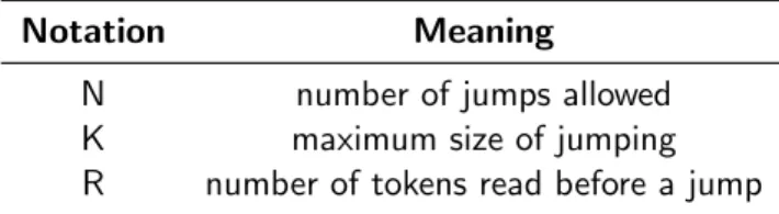
In LSTM-Jump, some hyperparameters defining the behavior of the subsampling scheme need to be defined ahead of time:

Notation Meaning

N number of jumps allowed K maximum size of jumping R number of tokens read before a jump

(21)

These hyperparameters define a reduced set of subsequences that the model can sample, instead of allowing the network to learn any arbitrary sampling scheme. This could lead to suboptimal sampling schemes and pushes some of the complexity towards the practitioner’s prior knowledge of the task. For instance, should the optimal policy consist in using every other sample, the model will be unable to learn the best sampling scheme if R= 2. Unlike LSTM-Jump, Skip RNN is not limited to a set of sample selection patterns which are predefined ahead of time.

(22)

Chapter 4

Model

An RNN takes an input sequence x = (x1, . . . , xT) and generates a state sequence s = (s1, . . . , sT) by iteratively applying a parametric state transition model S fromt= 1 toT:

st=S(st−1, xt) (4.1)

We augment the network with a binary state update gate,ut∈ {0,1}, selecting whether the state of the RNN will be updated or copied from the previous time step. At every time step t, the probability u˜t+1 ∈ [0,1] of performing a state update att+ 1 is emitted. The resulting architecture is depicted in Figure 4.1 and can be characterized as follows:

ut=fbinarize(˜ut) (4.2)

st=ut·S(st−1, xt) + (1−ut)·st−1 (4.3)

∆˜ut=σ(Wpst+bp) (4.4)

˜

ut+1=ut·∆˜ut+ (1−ut)·(˜ut+ min(∆˜ut,1−u˜t)) (4.5) where σ is the sigmoid function and fbinarize : [0,1] → {0,1} binarizes the input value. Should the network be composed of several layers, some columns of Wp can be fixed to 0 so that ∆˜ut depends only on the states of a subset of layers (see Section 5.5 for an example with two layers). We implementfbinarize as a deterministic step functionut=round(˜ut), although a stochastic sampling from a Bernoulli distributionut∼Bernoulli(˜ut) would be possible as well.

The model formulation implements the observation that the likelihood of requesting a new input increases with the number of consecutively skipped samples. Whenever a state update is omitted, the pre-activation of the state update gate for the following time step, u˜t+1, is incremented by ∆˜ut. On the other hand, if a state update is performed, the accumulated value is flushed andu˜t+1 = ∆˜ut.

The number of skipped time steps can be computed ahead of time. For the particular for-mulation used in this work, where fbinarizeis implemented by means of a rounding function, the number of skipped samples after performing a state update at time step tis given by:

(23)

f_binarize + S st ũ_t+1 σ Δũ_t u_t x_t 0 1 0 1 s_t-1 ũ_t (a) S s_t σ Δũ_t x_t s_t-1 ũ_t ũ_t+1 (b) x_t s_t-1 ũ_t s_t + ũ_t+1 σ Δũ_t (c) x_t s_t-1 ũ_t s_t Δũ_t-1 + ũ_t+1 Δũ_t (d)

Figure 4.1: Model architecture of the proposed Skip RNN.(a)Complete Skip RNN architecture, where the computation graph at time step t is conditioned on ut. (b) Architecture when the state is updated, i.e. ut= 1. (c) Architecture when the update step is skipped and the previous state is copied, i.e. ut = 0. (d) In practice, redundant computation is avoided by propagating ∆˜ut between time steps when ut= 0.

where n ∈ Z+_{. This enables more efficient implementations where no computation at all is} performed wheneverut= 0. These computational savings are possible because∆˜ut=σ(Wpst+ bp) = σ(Wpst−1 +bp) = ∆˜ut−1 when ut = 0 and there is no need to evaluate it again, as depicted in Figure 4.1d.

There are several advantages in reducing the number of RNN updates. From the computa-tional standpoint, fewer updates translates into fewer required sequential operations to process an input signal, leading to faster inference and reduced energy consumption. Unlike some other models that aim to reduce the average number of operations per step [41, 27], ours enables skipping steps completely. Replacing RNN updates with copy operations increases the memory of the network and its ability to model long term dependencies even for gated units, since the exponential memory decay observed in LSTM and GRU [41] is alleviated. During training, gra-dients are propagated through fewer updating time steps, providing faster convergence in some tasks involving long sequences. Moreover, the proposed model is orthogonal to recent advances in RNNs and could be used in conjunction with such techniques, e.g. normalization [12, 4], regularization [61, 33], variable computation [27, 41] or even external memory [21, 54].

(24)

4.1

Error gradients

The whole model is differentiable except forfbinarize, which outputs binary values. A common method for optimizing functions involving discrete variables is REINFORCE [55], although several estimators have been proposed for the particular case of neurons with binary outputs [7]. We select the straight-through estimator [24], which consists in approximating the step function by the identity when computing gradients during the backwards pass:

∂fbinarize(x)

∂x = 1 (4.7)

This yields a biased estimator that has proven more efficient than other unbiased but high-variance estimators such as REINFORCE [7] and has been successfully applied in different works [13, 11]. By using the straight-through estimator as the backwards pass forfbinarize, all the model parameters can be trained to minimize the target loss function with standard backpropagation and without defining any additional supervision or reward signal.

4.2

Limiting computation

The Skip RNN is able to learn when to update or copy the state without explicit information about which samples are useful to solve the task at hand. However, a different operating point on the trade-off between performance and number of processed samples may be required depending on the application, e.g. one may be willing to sacrifice a few accuracy points in order to run faster on machines with low computational power, or to reduce energy impact on portable devices. The proposed model can be encouraged to perform fewer state updates through additional loss terms, a common practice in neural networks with dynamically allocated computation [36, 38, 19, 27]. In particular, we will consider the introduction of a cost per sample:

Lbudget =λ· T

X

t=1

ut (4.8)

where Lbudget is the cost associated to a single sequence, λ is the cost per sample and T is the sequence length. This formulation bears a similarity to weight decay regularization, where the network is encouraged to slowly converge towards a solution where the norm of the weights is smaller. Similarly, in this case the network is encouraged to slowly converge towards a solution where fewer state updates are required.

Despite this formulation has been extensively studied in our experiments, different budget loss terms can be used depending on the application. For instance, a specific number of samples may be encouraged by applying anL1 orL2 loss between the target value and the number of updates per sequence, PT_t₌₁ut.

(25)

Chapter 5

Experimental Results

In the following sections, we investigate the advantages of adding the Skip RNN architecture to LSTMs and GRUs for a variety of tasks. Besides the evaluation metric for each task, we report the number of RNN state updates (i.e. the number of elements in the input sequence that are used by the model) as a measure of the computational load for each model. Unlike the wall clock time required by each model to process an input sequence, which we found to be highly dependent on the particular software implementation even for the baseline models, the number of RNN updates provides a meaningful measure of the inherently sequential operations in the computation graph. Since skipping an RNN update results in ignoring its corresponding input, we will refer to the number of updates and the number of used samples (i.e. elements in a sequence) interchangeably throughout this manuscript. For additional qualitative results, see Appendix A.

Training is performed with Adam optimizer [30], learning rate of 10−4_,_β1_{= 0}_.₉_,_β2_{= 0}_.₉₉₉ and= 10−8 _{on batches of 256 samples. Gradient clipping [44] with a threshold of 1 is applied} to all trainable variables. Bias bp in Equation 4.4 is initialized to 1, so that all samples are used at the beginning of training1. The initial hidden state s0 is learned during training, whereasu0˜ is set to a constant value of 1 in order to force the first update att= 1.

5.1

Adding Task

We revisit one of the original LSTM tasks [25], where the network is given a sequence of (value, marker) tuples. The desired output is the addition of the only two values that were marked with a 1, whereas those marked with a 0 need to be ignored. In particular, we follow the experimental setup by Neil et al. [41], where the first marker is randomly placed among the first 10% of samples (drawn with uniform probability) and the second one is placed among the last half of samples (drawn with uniform probability). This marker distribution yields sequences where at least 40% of the samples are distractors and provide no useful information at all. However, it is worth noting that in this task the risk of missing a marker is very large as compared to the benefits of working on shorter subsequences.

1

In practice, forcing the network to use all samples at the beginning of training improves its robustness against random initializations of its weights and increases the reproducibility of the presented experiments. A similar behavior was observed in other augmented RNN architectures such as Neural Stacks [22].

(26)

Model Task solved State updates

LSTM Yes 100.0%_±0.0%

Skip LSTM,λ= 0 Yes 81.1%_±3.6% Skip LSTM,λ= 10−5 _Yes _53.9_%_±_2.1_%

GRU Yes 100.0%_±0.0%

Skip GRU, λ= 0 Yes 97.9%_±3.2% Skip GRU, λ= 10−5 _Yes _50.7_%_±_2.6_%

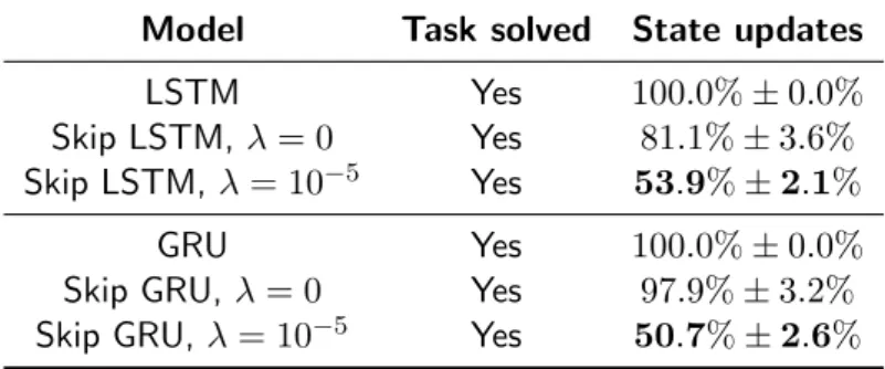
Table 5.1: Results for the adding task, displayed as mean_±std over four different runs. The task is considered to be solved if the MSE is at least two orders of magnitude below the variance of the output distribution.

We train RNN models with 110 units each on sequences of length 50, where the values are uniformly drawn from _U(₋0.5,0.5). The final RNN state is fed to a fully connected layer that regresses the scalar output. The whole model is trained to minimize the Mean Squared Error (MSE) between the output and the ground truth. We consider that a model is able to solve the task when its MSE on a held-out set of examples is at least two orders of magnitude below the variance of the output distribution. This criterion is a stricter version of the one followed in [25]. While all models learn to solve the task, results in Table 5.1 show that the Skip RNN models are able to do so with roughly half of the updates of their standard counterparts. Interestingly, Skip LSTM tends to skip more updates than the Skip GRU when no cost per sample is set, behavior that may be related to the lack of output gate in the latter. We hypothesize that there are two possible reasons why the output gate makes the LSTM more prone to skipping updates: (a) it introduces an additional source of memory decay, and (b) it allows to mask out some units in the cell state that may specialize in deciding when to update or copy, making the final regression layer agnostic to such process.

We observed that the models using fewer updates never miss any marker, since the penalization in terms of MSE would be very large (see Figure 5.1 for examples). These models learn to skip most of the samples in the 40% of the sequence where there are no markers. Moreover, most updates are skipped once the second marker is found, since all the relevant information in the sequence has been already seen. This last pattern provides evidence that the proposed models effectively learn to decide whether to update or copy the hidden state based on the input sequence, as opposed to learning biases in the dataset only. As a downside, Skip RNN models show some difficulties skipping a large number of updates at once, probably due to the cumulative nature of ˜

ut.

5.2

Frequency Discrimination Task

In this experiment, the network is trained to classify between sinusoids whose period is in range T _{∼ U}(5,6)milliseconds and those whose period is in rangeT _{∼ {}(1,5)_∪(6,100)_}milliseconds [41]. Every sine wave with periodT has a random phase shift drawn fromU(0, T). At every time step, the input to the network is a single scalar representing the amplitude of the signal. Since sinusoid are continuous signals, this tasks allows to study whether Skip RNNs converge to the same solutions when their parameters are fixed but the sampling period is changed. We study

(27)

0 10 20 30 40 50 time step 0 1 marker value 0 10 20 30 40 50 time step marker value

Figure 5.1: Sample usage examples for the Skip GRU with λ= 10−5 _{on the adding task. Red} dots indicate used samples, whereas blue ones are skipped.

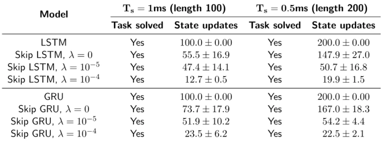
Model Ts=1ms (length 100) Ts=0.5ms (length 200) Task solved State updates Task solved State updates

LSTM Yes 100.0_±0.00 Yes 200.0_±0.00

Skip LSTM, λ= 0 Yes 55.5±16.9 Yes 147.9±27.0 Skip LSTM,λ= 10−5 _Yes ₄₇_.₄_±₁₄_.₁ _Yes ₅₀_.₇_±₁₆_.₈ Skip LSTM,λ= 10−4 _Yes ₁₂_.₇_±₀_.₅ _Yes ₁₉_.₉_±₁_.₅

GRU Yes 100.0_±0.00 Yes 200.0_±0.00

Skip GRU,λ= 0 Yes 73.7_±17.9 Yes 167.0_±18.3 Skip GRU, λ= 10−5 _Yes ₅₁_.₉_±₁₀_.₂ _Yes ₅₄_.₂_±₄_.₄ Skip GRU, λ= 10−4 _Yes ₂₃_.₅_±₆_.₂ _Yes ₂₂_.₅_±₂_.₁

Table 5.2: Results for the frequency discrimination task, displayed as mean_±std over four different runs. The task is considered to be solved if the classification accuracy is over 99%. Models with the same cost per sample (λ > 0) converge to a similar number of used samples under different sampling conditions.

two different sampling periods,Ts={0.5,1}milliseconds, for each set of hyperparameters. We train RNNs with 110 units each on input signals of 100 milliseconds. Batches are stratified, containing the same number of samples for each class, yielding a 50% chance accuracy. The last state of the RNN is fed into a 2-way classifier and trained with cross-entropy loss. We consider that a model is able to solve the task when it achieves an accuracy over 99% on a held-out set of examples.

Table 5.2 summarizes results for this task. When no cost per sample is set (λ = 0), the number of updates differ under different sampling conditions. We attribute this behavior to the potentially large number of local minima in the cost function, since there are numerous subsampling patterns for which the task can be successfully solved and we are not explicitly encouraging the network to converge to a particular solution. On the other hand, when λ > 0 Skip RNN models with the same cost per sample use roughly the same number of input samples even when the sampling frequency is doubled. This is a desirable property, since solutions are robust to oversampled input signals.

(28)

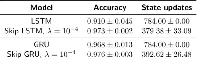
Model Accuracy State updates LSTM 0.910_±0.045 784.00_±0.00 Skip LSTM, λ= 10−4 ₀_.₉₇₃_±₀_.₀₀₂ ₃₇₉_.₃₈_±₃₃_.₀₉

GRU 0.968±0.013 784.00±0.00 Skip GRU,λ= 10−4 ₀_.₉₇₆_±₀_.₀₀₃ ₃₉₂_.₆₂_±₂₆_.₄₈

Table 5.3: Accuracy and used samples on the test set of MNIST after 600 epochs of training. Results are displayed asmean±stdover four different runs.

5.3

MNIST Classification from a Sequence of Pixels

The MNIST handwritten digits classification benchmark [35] is traditionally addressed with Convolutional Neural Networks (CNNs) that can efficiently exploit spatial dependencies through weight sharing. By flattening the28_×28 images into784-d vectors, however, it can be reformu-lated as a challenging task for RNNs where long term dependencies need to be leveraged [34]. We follow the standard data split and set aside 5,000 training samples for validation purposes. After processing all pixels with an RNN with 110 units, the last hidden state is fed into a linear classifier predicting the digit class. All models are trained for 600 epochs to minimize cross-entropy loss.

Table 5.3 summarizes classification results on the test set after 600 epochs of training. Skip RNNs are not only able to solve the task using fewer updates than their counterparts, but also show a lower variation among runs and train faster (see Figure 5.2). We hypothesize that skipping updates make the Skip RNNs work on shorter subsequences, simplifying the optimization process and allowing the networks to capture long term dependencies more easily. A similar behavior was observed for Phased LSTM, where increasing the sparsity of cell updates accelerates training for very long sequences [41].

Sequences of pixels can be reshaped back into 2D images, allowing to visualize the samples used by the RNNs as a sort of hard visual attention model [57]. Examples such as the ones depicted in Figure 5.3 (top) show how the model learns to skip pixels that are not discriminative, such as the padding regions in the top and bottom of images. Similarly to the qualitative results for the adding task (Section 5.1), attended samples vary depending on the particular input being given to the network.

With the aim of observing how the attention model changes with the task, we train Skip LSTM (λ= 10−4_{) models on two subsets of MNIST. We select pairs of visually similar digits:} classes 1 and 7 (MNIST-17) and classes 5 and 6 (MNIST-56). Figure 5.3 (middle and bottom) shows how the network is able to find the most discriminative region for each pair of digits and mostly ignores the rest of the image. These regions differ from the ones attended by the model trained on the full dataset, depicted in Figure 5.3 (top).

5.4

Sentiment Analysis on IMDB

The IMDB dataset [37] contains 25,000 training and 25,000 testing movie reviews annotated into two classes, positive and negative sentiment, with an approximate average length of 240

(29)

0

100

200

300

400

500

600

Epochs

20

40

60

80

100

Accuracy (%)

GRU

Skip GRU, = 10

4

Figure 5.2: Accuracy evolution during training on the validation set of MNIST. The Skip GRU exhibits lower variance and faster convergence than the baseline GRU. A similar behavior is observed for LSTM and Skip LSTM, but omitted for clarity. Shading shows maximum and minimum over 4 runs, while dark lines indicate the mean.

Figure 5.3: Sample usage examples for the Skip LSTM with λ= 10−4 _{on the test set of MNIST} (top), MNIST-17 (middle) and MNIST-56 (bottom). Red pixels are used, whereas blue ones are skipped.

(30)

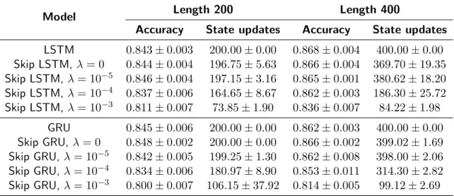
Model Length 200 Length 400

Accuracy State updates Accuracy State updates LSTM 0.843_±0.003 200.00_±0.00 0.868_±0.004 400.00_±0.00 Skip LSTM, λ= 0 0.844_±0.004 196.75_±5.63 0.866_±0.004 369.70_±19.35 Skip LSTM,λ= 10−5 ₀_.₈₄₆_±₀_.₀₀₄ ₁₉₇_.₁₅_±₃_.₁₆ ₀_.₈₆₅_±₀_.₀₀₁ ₃₈₀_.₆₂_±₁₈_.₂₀ Skip LSTM,λ= 10−4 ₀_.₈₃₇_±₀_.₀₀₆ ₁₆₄_.₆₅_±₈_.₆₇ ₀_.₈₆₂_±₀_.₀₀₃ ₁₈₆_.₃₀_±₂₅_.₇₂ Skip LSTM,λ= 10−3 ₀_.₈₁₁_±₀_.₀₀₇ ₇₃_.₈₅_±₁_.₉₀ ₀_.₈₃₆_±₀_.₀₀₇ ₈₄_.₂₂_±₁_.₉₈ GRU 0.845_±0.006 200.00_±0.00 0.862_±0.003 400.00_±0.00 Skip GRU,λ= 0 0.848±0.002 200.00±0.00 0.866±0.002 399.02±1.69 Skip GRU, λ= 10−5 ₀_.₈₄₂_±₀_.₀₀₅ ₁₉₉_.₂₅_±₁_.₃₀ ₀_.₈₆₂_±₀_.₀₀₈ ₃₉₈_.₀₀_±₂_.₀₆ Skip GRU, λ= 10−4 ₀_.₈₃₄_±₀_.₀₀₆ ₁₈₀_.₉₇_±₈_.₉₀ ₀_.₈₅₃_±₀_.₀₁₁ ₃₁₄_.₃₀_±₂_.₈₂ Skip GRU, λ= 10−3 ₀_.₈₀₀_±₀_.₀₀₇ ₁₀₆_.₁₅_±₃₇_.₉₂ ₀_.₈₁₄_±₀_.₀₀₅ ₉₉_.₁₂_±₂_.₆₉

Table 5.4: Accuracy and used samples on the test set of IMDB for different sequence lengths. Results are displayed asmean±stdover four different runs.

words per review. We set aside15%of training data for validation purposes. Words are embedded into 300-d vector representations before being fed to an RNN with 128 units. The embedding matrix is initialized using pre-trained word2vec2 embeddings [39] when available, or random vectors drawn from_U(₋0.25,0.25)otherwise [29]. Dropout with rate0.2is applied between the last RNN state and the classification layer in order to reduce overfitting. We evaluate the models on sequences of length 200 and 400 by cropping longer sequences and padding shorter ones [59]. Results on the test are reported in Table 5.4. In a task where it is hard to predict which input tokens will be discriminative, the Skip RNN models are able to achieve similar accuracy rates to the baseline models while reducing the number of required updates. These results highlight the trade-off between accuracy and the available computational budget, since a larger cost per sample results in lower accuracies. However, allowing the network to select which samples to use instead of cropping sequences at a given length boosts performance, as observed for the Skip LSTM (length 400,λ= 10−4_{), which achieves a higher accuracy than the baseline LSTM (length 200)} while seeing roughly the same number of words per review. A similar behavior can be seen for the Skip RNN models withλ= 10−3_{, where allowing them to select words from longer reviews} boosts classification accuracy while using a comparable number of tokens per sequence.

5.5

Action classification on UCF-101

One of the most accurate and scalable pipelines for video analysis consists in extracting frame level features with a CNN and modeling their temporal evolution with an RNN [16, 60]. Videos are commonly recorded at high sampling rates, rapidly generating long sequences with strong temporal redundancy that are challenging for RNNs. Moreover, processing frames with a CNN is computationally expensive and may become prohibitive for high framerates. These issues have been alleviated in previous works by using short clips [16] or by downsampling the original data in order to cover long temporal spans without increasing the sequence length excessively [60]. Instead of addressing the long sequence problem at the input data level, we train RNN models

2

(31)

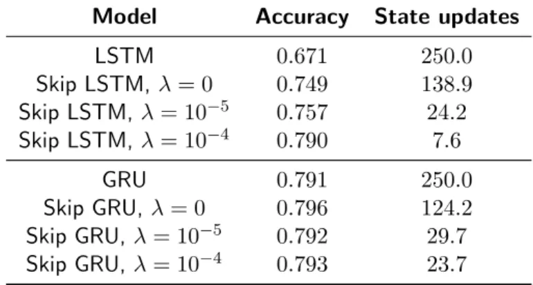
Model Accuracy State updates LSTM 0.671 250.0 Skip LSTM,λ= 0 0.749 138.9 Skip LSTM,λ= 10−5 ₀_.₇₅₇ ₂₄_.₂ Skip LSTM,λ= 10−4 ₀_.₇₉₀ ₇_.₆ GRU 0.791 250.0 Skip GRU, λ= 0 0.796 124.2 Skip GRU,λ= 10−5 ₀_.₇₉₂ ₂₉_.₇ Skip GRU,λ= 10−4 ₀_.₇₉₃ ₂₃_.₇

Table 5.5: Accuracy and used samples on the validation set of UCF-101 (split 1).

0

50

100

150

200

250

300

Epochs

0

20

40

60

80

Accuracy (%)

LSTM

Skip LSTM, = 0

Skip LSTM, = 10

5

Skip LSTM, = 10

4

Figure 5.4: Accuracy evolution during the first 300 training epochs on the validation set of UCF-101 (split 1). Skip LSTM models converge much faster than the baseline LSTM.

using long frame sequences without downsampling and let the network learn which frames need to be used.

UCF-101 [51] is a dataset containing 13,320 trimmed videos belonging to 101 different action categories. We use 10 seconds of video sampled at 25fps, cropping longer ones and padding shorter examples with empty frames. Activations in the Global Average Pooling layer from a ResNet-50 [23] CNN pretrained on the ImageNet dataset [15] are used as frame level features, which are fed into two stacked RNN layers with 512 units each. The weights in the CNN are not tuned during training to reduce overfitting. The hidden state in the last RNN layer is used to compute the update probability for the Skip RNN models.

We evaluate the different models on the first split of UCF-101 and report results in Table 5.5. Skip RNN models do not only improve the classification accuracy with respect to the baseline, but require very few updates to do so. We argue that this is possible due to the low motion between consecutive frames resulting in frame level features with high temporal redundancy [48]. Moreover, Figure 5.4 shows how models performing fewer updates converge faster thanks to the gradients being preserved during longer spans when training with backpropagation through time.

(32)

Chapter 6

Budget

We estimate that the overall GPU usage for the experiments presented in this thesis is roughly 2,880 hours. However, these represent a small fraction of the overall GPU usage, since alternative formulations, hyperparameter settings and debugging experiments were run before achieving the final results included in this document. For the purpose of cost estimation, we assume that the presented experiments comprise around a 20% of the overall computation, thus leading to roughly 14,400 hours of GPU usage. We compute the computation cost based on Amazon Web Services (AWS) rates1 for p2.xlarge instances with one NVIDIA K80 each, which is a dual-GPU and allows to run sets of two experiments in parallel.

The length of the project was 24 weeks. Assuming a commitment of 40 weekly hours and that each advisor spent an average of 1h per week on meetings, the complete costs for the project are the following:

Amount Cost/hour Time Total

AWSp2.xlarge instance 0.5 $0.90 14,400h $6,480

Junior engineer 1 $8.00 960h $7,680

Senior engineer 4 $30.00 24h $2,880

Other equipment - - - $4,000

Total $21,040

Table 6.1: Cost of the project. Other equipment includes campus services, office supplies and hardware, e.g. the employed laptop and auxiliary monitor.

1

(33)

Chapter 7

Conclusion and Future Work

We presented Skip RNN as an extension to existing recurrent architectures enabling them to skip state updates, thus reducing the number of sequential operations in the computation graph. Unlike previous approaches, all parameters in Skip RNN are trained with backpropagation without requiring to introduce task-dependent modifications. Experiments conducted on LSTM and GRU showed how Skip RNNs match the performance of baseline models while relaxing their computational requirements. Evaluation is performed on a broad set of tasks and datasets involving synthetic data, images, text and video. Skip RNNs provide a faster and more stable training for long sequences and complex models, likely due to gradients being backpropagated through fewer time steps resulting in a simpler optimization task. Moreover, the introduced computational savings are better suited for modern hardware than those methods that reduce the number of computations required at each time step [31, 41, 11].

The presented results motivate several new research directions towards designing efficient RNN architectures. Introducing stochasticity in neural network training has proven beneficial [52, 33], so that replacing the deterministic rounding operation with a stochastic sampling is a natural extension to the current formulation. This may improve generalization while allowing the model to escape poor local minima more easily. The loss term penalizing the number of updates is an important element in the performance of Skip RNN and different formulations can be tailored for specific tasks. For instance, the cost could increase at each time step to encourage the network to emit a decision earlier [1], or a particular number of updates can be enforced if such information is available. Finally, understanding and analyzing the patterns followed by the model when deciding whether to update or copy the RNN state may provide insight for developing better and more efficient architectures.

This project was aimed at designing a recurrent architecture capable of skipping state updates and showing its advantages in a series of tasks. Once the formulation is mature enough and has been proven effective, future work should focus on developing efficient implementations pushing the limits in terms of wall clock time. This may include the development of low level CUDA kernels that speedup the execution of Skip RNN models, as well as porting the code to a framework based on dynamic computational graphs (e.g. PyTorch1, DyNet2, Chainer3). The latter are more suitable for the problem at hand than frameworks based on static computation graphs, since the

1 http://www.pytorch.org/ 2 https://github.com/clab/dynet/ 3 https://chainer.org/

(34)

actual computation graph is conditioned on the model outputs at each time step and cannot be completely defined before being run.

(35)

Bibliography

[1] Mohammad Sadegh Aliakbarian, Fatemehsadat Saleh, Mathieu Salzmann, Basura Fernando, Lars Petersson, and Lars Andersson. Encouraging LSTMs to anticipate actions very early. arXiv preprint arXiv:1703.07023, 2017.

[2] Amjad Almahairi, Nicolas Ballas, Tim Cooijmans, Yin Zheng, Hugo Larochelle, and Aaron Courville. Dynamic capacity networks. InICML, 2016.

[3] Jimmy Ba, Volodymyr Mnih, and Koray Kavukcuoglu. Multiple object recognition with visual attention. arXiv preprint arXiv:1412.7755, 2014.

[4] Jimmy Lei Ba, Jamie Ryan Kiros, and Geoffrey E Hinton. Layer normalization. arXiv preprint arXiv:1607.06450, 2016.

[5] Dzmitry Bahdanau, Kyunghyun Cho, and Yoshua Bengio. Neural machine translation by jointly learning to align and translate. InICLR, 2015.

[6] Yoshua Bengio. Deep learning of representations: Looking forward. In SLSP, 2013.

[7] Yoshua Bengio, Nicholas L´eonard, and Aaron Courville. Estimating or propagating gradients through stochastic neurons for conditional computation. arXiv preprint arXiv:1308.3432, 2013.

[8] Yoshua Bengio, Patrice Simard, and Paolo Frasconi. Learning long-term dependencies with gradient descent is difficult. IEEE Transactions on Neural Networks, 1994.

[9] Subhabrata Bhattacharya, Felix X Yu, and Shih-Fu Chang. Minimally needed evidence for complex event recognition in unconstrained videos. In ICMR, 2014.

[10] Kyunghyun Cho, Bart Van Merri¨enboer, Caglar Gulcehre, Dzmitry Bahdanau, Fethi Bougares, Holger Schwenk, and Yoshua Bengio. Learning phrase representations using rnn encoder-decoder for statistical machine translation. InEMNLP, 2014.

[11] Junyoung Chung, Sungjin Ahn, and Yoshua Bengio. Hierarchical multiscale recurrent neural networks. In ICLR, 2017.

[12] Tim Cooijmans, Nicolas Ballas, César Laurent, Ç a˘glar Gül¸cehre, and Aaron Courville. Re-current batch normalization. In ICLR, 2017.

[13] Matthieu Courbariaux, Itay Hubara, Daniel Soudry, Ran El-Yaniv, and Yoshua Bengio. Bi-narized neural networks: Training deep neural networks with weights and activations con-strained to+ 1 or-1. arXiv preprint arXiv:1602.02830, 2016.

[14] Andrew Davis and Itamar Arel. Low-rank approximations for conditional feedforward com-putation in deep neural networks. arXiv preprint arXiv:1312.4461, 2013.

(36)

[15] Jia Deng, Wei Dong, Richard Socher, Li-Jia Li, Kai Li, and Li Fei-Fei. ImageNet: A large-scale hierarchical image database. InCVPR, 2009.

[16] Jeffrey Donahue, Lisa Anne Hendricks, Sergio Guadarrama, Marcus Rohrbach, Subhashini Venugopalan, Kate Saenko, and Trevor Darrell. Long-term recurrent convolutional networks for visual recognition and description. InCVPR, 2015.

[17] Michael Figurnov, Maxwell D Collins, Yukun Zhu, Li Zhang, Jonathan Huang, Dmitry Vetrov, and Ruslan Salakhutdinov. Spatially adaptive computation time for residual net-works. In CVPR, 2017.

[18] Ian Goodfellow, Yoshua Bengio, and Aaron Courville. Deep learning. MIT press, 2016. [19] Alex Graves. Adaptive computation time for recurrent neural networks. arXiv preprint

arXiv:1603.08983, 2016.

[20] Alex Graves, Abdel-rahman Mohamed, and Geoffrey Hinton. Speech recognition with deep recurrent neural networks. In ICASSP, 2013.

[21] Alex Graves, Greg Wayne, and Ivo Danihelka. Neural turing machines. arXiv preprint arXiv:1410.5401, 2014.

[22] Edward Grefenstette, Karl Moritz Hermann, Mustafa Suleyman, and Phil Blunsom. Learning to transduce with unbounded memory. InNIPS, 2015.

[23] Kaiming He, Xiangyu Zhang, Shaoqing Ren, and Jian Sun. Deep residual learning for image recognition. In CVPR, 2016.

[24] Geoffrey Hinton. Neural networks for machine learning. Coursera video lectures, 2012. [25] Sepp Hochreiter and J¨urgen Schmidhuber. Long short-term memory. Neural computation,

1997.

[26] Gao Huang, Yu Sun, Zhuang Liu, Daniel Sedra, and Kilian Q Weinberger. Deep networks with stochastic depth. In ECCV, 2016.

[27] Yacine Jernite, Edouard Grave, Armand Joulin, and Tomas Mikolov. Variable computation in recurrent neural networks. InICLR, 2017.

[28] Andrej Karpathy, George Toderici, Sanketh Shetty, Thomas Leung, Rahul Sukthankar, and Li Fei-Fei. Large-scale video classification with convolutional neural networks. In CVPR, 2014.

[29] Yoon Kim. Convolutional neural networks for sentence classification. In EMNLP, 2014. [30] Diederik Kingma and Jimmy Ba. Adam: A method for stochastic optimization. arXiv

preprint arXiv:1412.6980, 2014.

[31] Jan Koutnik, Klaus Greff, Faustino Gomez, and Juergen Schmidhuber. A clockwork rnn. In ICML, 2014.

[32] Alex Krizhevsky, Ilya Sutskever, and Geoffrey E Hinton. Imagenet classification with deep convolutional neural networks. InNIPS, 2012.

[33] David Krueger, Tegan Maharaj, J´anos Kram´ar, Mohammad Pezeshki, Nicolas Ballas, Nan Rosemary Ke, Anirudh Goyal, Yoshua Bengio, Hugo Larochelle, Aaron Courville, et al. Zoneout: Regularizing rnns by randomly preserving hidden activations. In ICLR, 2017.

(37)

[34] Quoc V Le, Navdeep Jaitly, and Geoffrey E Hinton. A simple way to initialize recurrent networks of rectified linear units. arXiv preprint arXiv:1504.00941, 2015.

[35] Yann LeCun, L´eon Bottou, Yoshua Bengio, and Patrick Haffner. Gradient-based learning applied to document recognition. Proceedings of the IEEE, 1998.

[36] Lanlan Liu and Jia Deng. Dynamic deep neural networks: Optimizing accuracy-efficiency trade-offs by selective execution. arXiv preprint arXiv:1701.00299, 2017.

[37] Andrew L Maas, Raymond E Daly, Peter T Pham, Dan Huang, Andrew Y Ng, and Christo-pher Potts. Learning word vectors for sentiment analysis. In ACL, 2011.

[38] Mason McGill and Pietro Perona. Deciding how to decide: Dynamic routing in artificial neural networks. In ICML, 2017.

[39] Tomas Mikolov, Ilya Sutskever, Kai Chen, Greg S Corrado, and Jeff Dean. Distributed representations of words and phrases and their compositionality. InNIPS, 2013.

[40] Volodymyr Mnih, Nicolas Heess, Alex Graves, et al. Recurrent models of visual attention. In NIPS, 2014.

[41] Daniel Neil, Michael Pfeiffer, and Shih-Chii Liu. Phased LSTM: accelerating recurrent network training for long or event-based sequences. InNIPS, 2016.

[42] Christopher Olah. Understanding LSTM networks. http://colah.github.io/posts/ 2015-08-Understanding-LSTMs/, 2015.

[43] Aaron van den Oord, Sander Dieleman, Heiga Zen, Karen Simonyan, Oriol Vinyals, Alex Graves, Nal Kalchbrenner, Andrew Senior, and Koray Kavukcuoglu. Wavenet: A generative model for raw audio. arXiv preprint arXiv:1609.03499, 2016.

[44] Razvan Pascanu, Tomas Mikolov, and Yoshua Bengio. On the difficulty of training recurrent neural networks. In ICML, 2013.

[45] Colin Raffel and Dieterich Lawson. Training a subsampling mechanism in expectation. In ICLR Workshop Track, 2017.

[46] Frank Rosenblatt. The perceptron: A probabilistic model for information storage and orga-nization in the brain. Psychological review, 1958.

[47] Noam Shazeer, Azalia Mirhoseini, Krzysztof Maziarz, Andy Davis, Quoc Le, Geoffrey Hinton, and Jeff Dean. Outrageously large neural networks: The sparsely-gated mixture-of-experts layer. In ICLR, 2017.

[48] Evan Shelhamer, Kate Rakelly, Judy Hoffman, and Trevor Darrell. Clockwork convnets for video semantic segmentation. arXiv preprint arXiv:1608.03609, 2016.

[49] Gunnar A Sigurdsson, Xinlei Chen, and Abhinav Gupta. Learning visual storylines with skipping recurrent neural networks. In ECCV, 2016.

[50] David Silver, Aja Huang, Chris J Maddison, Arthur Guez, Laurent Sifre, George Van Den Driessche, Julian Schrittwieser, Ioannis Antonoglou, Veda Panneershelvam, Marc Lanc-tot, et al. Mastering the game of go with deep neural networks and tree search. Nature, 2016.

[51] Khurram Soomro, Amir Roshan Zamir, and Mubarak Shah. Ucf101: A dataset of 101 human actions classes from videos in the wild. arXiv preprint arXiv:1212.0402, 2012.

(38)

[52] Nitish Srivastava, Geoffrey Hinton, Alex Krizhevsky, Ilya Sutskever, and Ruslan Salakhutdi-nov. Dropout: A simple way to prevent neural networks from overfitting. The Journal of Machine Learning Research, 2014.

[53] Christian Szegedy, Wei Liu, Yangqing Jia, Pierre Sermanet, Scott Reed, Dragomir Anguelov, Dumitru Erhan, Vincent Vanhoucke, and Andrew Rabinovich. Going deeper with convolu-tions. InCVPR, 2015.

[54] Jason Weston, Sumit Chopra, and Antoine Bordes. Memory networks. arXiv preprint arXiv:1410.3916, 2014.

[55] Ronald J Williams. Simple statistical gradient-following algorithms for connectionist rein-forcement learning. Machine learning, 1992.

[56] Yonghui Wu, Mike Schuster, Zhifeng Chen, Quoc V Le, Mohammad Norouzi, Wolfgang Macherey, Maxim Krikun, Yuan Cao, Qin Gao, Klaus Macherey, et al. Google’s neural machine translation system: Bridging the gap between human and machine translation. arXiv preprint arXiv:1609.08144, 2016.

[57] Kelvin Xu, Jimmy Ba, Ryan Kiros, Kyunghyun Cho, Aaron Courville, Ruslan Salakhudinov, Rich Zemel, and Yoshua Bengio. Show, attend and tell: Neural image caption generation with visual attention. InICML, 2015.

[58] Serena Yeung, Olga Russakovsky, Greg Mori, and Li Fei-Fei. End-to-end learning of action detection from frame glimpses in videos. In CVPR, 2016.

[59] Adams Wei Yu, Hongrae Lee, and Quoc V Le. Learning to skim text. In ACL, 2017. [60] Joe Yue-Hei Ng, Matthew Hausknecht, Sudheendra Vijayanarasimhan, Oriol Vinyals, Rajat

Monga, and George Toderici. Beyond short snippets: Deep networks for video classification. In CVPR, 2015.

[61] Wojciech Zaremba, Ilya Sutskever, and Oriol Vinyals. Recurrent neural network regulariza-tion. In ICLR, 2015.

(39)

Appendix A

Qualitative results

(40)

A.1

Adding task

0 10 20 30 40 50 time step 0 1 marker value 0 10 20 30 40 50 time step 0 1 marker value 0 10 20 30 40 50 time step 0 1 marker value 0 10 20 30 40 50 time step 0 1 marker value 0 10 20 30 40 50 time step 0 1 marker value 0 10 20 30 40 50 time step 0 1 marker value 0 10 20 30 40 50 time step 0 1 marker value 0 10 20 30 40 50 time step 0 1 marker value 0 10 20 30 40 50 time step 0 1 marker value 0 10 20 30 40 50 time step 0 1 marker value

Figure A.1: Sample usage examples for the Skip GRU with λ= 10−5 _{on the adding task. Red} dots indicate used samples, whereas blue ones are skipped.

(41)

A.2

Frequency discrimination task

0 25 50 75 100 125 150 175 200 sample 1 0 1 amplitude 0 25 50 75 100 125 150 175 200 sample 1 0 1 amplitude 0 25 50 75 100 125 150 175 200 sample 1 0 1 amplitude 0 25 50 75 100 125 150 175 200 sample 1 0 1 amplitude 0 25 50 75 100 125 150 175 200 sample 1 0 1 amplitude 0 25 50 75 100 125 150 175 200 sample 1 0 1 amplitude 0 25 50 75 100 125 150 175 200 sample 1 0 1 amplitude 0 25 50 75 100 125 150 175 200 sample 1 0 1 amplitude 0 25 50 75 100 125 150 175 200 sample 1 0 1 amplitude 0 25 50 75 100 125 150 175 200 sample 1 0 1 amplitude

Figure A.2: Sample usage examples for the Skip LSTM withλ= 10−4 _{on the frequency} discrim-ination task with Ts = 0.5ms. Red dots indicate used samples, whereas blue ones are skipped. The network learns that using the first samples is enough to classify the frequency of the sine waves, in contrast to a uniform downsampling that may result in aliasing.

(42)