Design of Near Optimal Decision Rules in Multistage Adaptive
Mixed-Integer Optimization
Dimitris Bertsimas
∗Angelos Georghiou
†September 2, 2014
Abstract
In recent years, decision rules have been established as the preferred solution method for address-ing computationally demandaddress-ing, multistage adaptive optimization problems. Despite their success, existing decision rules (a) are typically constrained by their a priori design and (b) do not incor-porate in their modeling adaptive binary decisions. To address these problems, we first derive the structure for optimal decision rules involving continuous and binary variables as piecewise linear and piecewise constant functions, respectively. We then propose a methodology for the optimal design of such decision rules that have finite number of pieces and solve the problem using mixed-integer optimization. We demonstrate the effectiveness of the proposed methods in the context of two multi-stage inventory control problems. We provide global lower bounds and show that our approach is (i) practically tractable and (ii) provides high quality solutions that outperform alternative methods. Keywords. Adaptive Optimization, Decision Rules, Mixed-integer optimization.
1
Introduction
Robust optimization has emerged as the leading modeling paradigm for optimization problems under uncertainty. Its success stems from its ability to immunize problems against perturbations in model
parameters, while preserving computational tractability, see Ben-Tal et al. [8] and Bertsimas and Sim
[14]. The classical robust optimization framework involves only here-and-now decisions, i.e., decisions
that must be selected before any of the uncertain parameters are observed. In recent years, adaptive robust optimization problems have attracted considerable interest. Such problems incorporate additional
∗Sloan School of Management and Operations Research Center, Massachusetts Institute of Technology, USA, E-mail: [email protected].
adaptive,wait-and-see decisions, which can be chosen after the parameter realizations are revealed. As
such, thesedecision rules are modeled as functions of the observed uncertain parameter realizations.
Adaptive optimization problems have been shown to be in general computationally intractable from a theoretical point of view, see Shapiro and Nemirovski [33]. A drastic but very effective simplification
in gaining computational tractability proposed in Ben-Talet al.[6], is to restrict the space of admissible
adaptive continuous decisions to those that admit a linear structure with respect to the random
param-eters. Specifically, given uncertainty ξ∈Ξ, the linear decision rule for an adaptive continuous variable
x(∙) is given by x(ξ) =x>ξ,ξ∈Ξ ⊆Rk. This linear decision rule has attracted considerable interest
in recent years, since its simple structure enables scalability to multistage models. Even though linear decision rules are known to be optimal for the linear quadratic regulator problem, see Anderson and
Moore [1], some one-dimensional robust control problems, see Bertsimas et al. [12], and some vehicle
routing problems, see Gounaris et al. [26], decision rules generically sacrifice a significant amount of
optimality in return for scalability. Indeed, Bertsimas and Goyal [11] have shown that the worst-case
cost associated with linear decision rules can beO(√k) suboptimal when applied to two-stage robust
op-timization problems withkuncertain parameters. The aforementioned work also shows that the optimal
decision rule for adaptive optimization problems is piecewise linear. This motivates the use of non-linear decision rules.
There is a plethora of non-linear decision rules appearing in the literature. Under a non-linear
decision rule, the adaptive decision x(∙) is given by x(ξ) = x>L(ξ), where L : Rk → Rk0, k ≤ k0,
is a non-linear operator, mapping the uncertain vector ξ to L(ξ) in a higher dimensional space L(Ξ).
Using the re-parameterization ξ0 = L(ξ), the adaptive decision rule x(ξ) = x>L(ξ) can be expressed
as a linear decision rule x(ξ0) = x>ξ0 for all ξ0 ∈ L(Ξ). The choice of the non-linear operator L(∙)
defines the non-linear structure of the decision rule. This formulation was first introduced by Chen and Zhang [21] creating simple piecewise linear decision rule structures. The framework was later extended
to cover general non-linear decision rules by Goh and Sim [24] and Georghiou et al. [23] in the realm
of stochastic programming. Bertsimaset al.[13] also proposed the use of polynomial decision rules for
adaptive robust optimization problems, an idea that was later refined by Bampou and Kuhn [3] in the context of stochastic programming. The strict advantage of the aforementioned approximations is that the resulting decision rule problems can be cast as conic optimization problems, whose size grows only polynomially with the input parameters. Nevertheless, there are two main disadvantages associated with
these non-linear decision rules: (i) The non-linear structure of the decision ruleL(∙) needs to be decided
a priori by the user; (ii) An exact reformulation of the decision rule problem into a finite dimensional
conic optimization problem can only be done efficiently for certain classes of non-linear decision rules
the choices of admissible decision rules, and can lead to the same worst-case performance as with linear decision rules.
In contrast to the large effort dedicated in developing decision rules for continuous decisions, very little effort is devoted in developing approximations for binary adaptive decisions. In most of the literature, all binary decisions are treated as here-and-now decisions leading to conservative estimates for the optimal solution. To the best of our knowledge, the work of Bertsimas and Caramanis in [10] is the only framework that can address the binary decisions in an adaptive robust optimization setting. To simulate the recourse nature of the binary decisions, the authors proposed to partition the uncertainty set into finite subsets, assigning a binary decision for each subset. Although this idea is very effective when the adaptive problem in hand has a small number of time stages, the exponential growth in the number of binary decisions and constraints renders the method unsuitable for multistage problems with large number of stages.
The goal of this paper is to design piecewise linear and piecewise constant decision rules for continuous and binary decisions, respectively, in the context of multistage adaptive optimization problems. The proposed decision rules overcome the shortfalls of existing approaches, while maintaining in part the desirable tractability properties of existing methods. The main contributions of this paper may be summarized as follows.
1. We derive the structure for the optimal decision rules involving both continuous and binary variables as piecewise linear and piecewise constant functions, respectively.
2. We propose a methodology for the optimal design of such piecewise linear continuous and piecewise linear binary decision rules that have fixed number of pieces. To the best of our knowledge, this is the first decision rule that can address binary adaptive decisions. In contrast with the non-linear continuous decision rules in the literature, the structure of the proposed decision rules is not decided a priori, but rather is decided endogenously through the solution of a sequence of mixed-integer optimization problems.
3. We demonstrate the effectiveness of the proposed methods in the context of two multistage
inven-tory control problems. We provide global lower bounds using the approach in Hadjiyiannis et al.
[27] and show that our approach is (i) practically tractable and (ii) provides high quality solutions
that outperform alternative methods.
The rest of this paper is organized as follows. In Section 2, we outline our approach for continuous and binary adaptive decision in the context of one-stage adaptive optimization problems involving only
In Section 4, we extent the proposed approach to multistage adaptive optimization problems and in Section 5, we present our computational results. Finally, Section 6 provides some concluding remarks.
Notation We denote scalar quantities by lowercase, non-bold face symbols and vector quantities by
lowercase, boldface symbols, e.g., x∈ Rand x∈ Rn, respectively. Similarly, scalar and vector valued
functions will be denoted by, x(∙)∈Rand x(∙)∈Rn, respectively. Matrices are denoted by uppercase
symbols , e.g., A∈Rn×m. Vectore
∈Rk denotes the vector of ones. We denote by
Rthe space of all
real-valued functions from Rk toRand
Bthe space of binary functions from Rk to
{0,1}.
2
Design of Piecewise Linear Decision Rules
In this section, we present our approach for one-stage adaptive optimization problems. Given matrices A∈Rm×n, B
∈Rm×q, C
∈Rm×k, vectors c
∈Rn,d
∈Rq and an uncertainty set Ξ for the uncertain
quantityξ∈Rk, we are interested to choose functions x(
∙) = (x1(∙), . . . , xn(∙))>, xi(∙)∈ R andy(∙) = (y1(∙), . . . , yq(∙))>, yi(∙)∈ Bin order to solve: minimize max ξ ∈Ξ c >x(ξ) +d>y(ξ) subject to xi(∙)∈ R, i= 1, . . . , n, yi(∙)∈ B, i= 1, . . . , q, Ax(ξ) +By(ξ)≤Cξ ∀ξ∈Ξ. (1)
Here, we assume that Problem (1) has a non-empty and bounded feasible region and the uncertainty set Ξ is a nonempty, convex and compact polyhedron
Ξ =ξ∈Rk :Wξ
≥g, ξ1= 1 , (2)
whereW ∈Rl×k andg
∈Rl. The parameterξ
1is set equal to 1 without loss of generality as it allows us
to represent affine functions of the non-degenerate outcomes (ξ2, . . . , ξk) in a compact manner as linear
functions ofξ= (ξ1, . . . , ξk).
Problem (1) involves a continuum of decision variables and inequality constraints. Therefore, in order to make the problem amenable to numerical solutions, there is a need for suitable functional
2.1
Design of Piecewise Linear Decision Rules for Real-Valued Decisions
To present our approach we consider first a special case of Problem (1) involving only real-valued recourse decisions: minimize max ξ ∈Ξ c >x(ξ) subject to xi(∙)∈ R, i= 1, . . . , n, Ax(ξ)≤Cξ ∀ξ∈Ξ. (3)
Bemporadet al.[4] showed that the optimal decision rules for Problem (3) are piecewise linear continuous
functions.
LetPC be the space of piecewise linear continuous functions from Rk toRthat admit the following
structure:
x(ξ) = max{x>1ξ, . . . ,x>Pξ} −max{x>1ξ, . . . ,x>Pξ}, (4)
for someP ∈N+ andxp,xp∈Rk, p∈ P :={1, . . . , P}.
Theorem 1 Every piecewise linear continuous function defined over a compact set Ξis an element ofPC.
Proof Given any piecewise linear convex function x : Rk → R, it can be written as the point-wise
supremum of a finite collection ofP linear functions:
x(ξ) = sup
p=1,...,P
x>
pξ,
for some P ∈ N+ and xp ∈ Rk. Since the uncertainty set Ξ in (3) is compact, we can replace the
supremum with the maximum operator, thus verifying that any piecewise linear convex function can be
written in the formx(ξ) = max{x>
1ξ, . . . ,x>Pξ}.
Hempel et al.[28, Lemma 4] states that for every piecewise linear continuous function x: Rk →R
defined over a convex polyhedral Ξ, there existsP ∈N+ and two piecewise linear continuous and convex
functionsx(ξ) = max{x>
1ξ, . . . ,x>Pξ}andx(ξ) = max{x>1ξ, . . . ,x>Pξ}such thatx(ξ) =x(ξ)−x(ξ). This
verifies that the space PC coincides with the space of all piecewise linear continuous functions defined
over a compact set Ξ.
The implication of Theorem 1 is that for every piecewise linear continuous function, there exists
P ∈ N+ such that the function can be written in the form (4). Since the optimal decision rules for
Problem (3) are piecewise linear continuous functions, see [4, Theorem 2], the optimal solution of Problem
(3) is an element of PC. Nevertheless, it will be computationally intractable to optimize over decisions
that have arbitrarily many linear pieces. To this end, we restrict the space of admissible solutions from
linear piecesP ∈N+is fixed. This functional restriction yields the following semi-infinite problem, which
for fixedP, involves only a finite number of decision variables, and an infinite number of constraints:
minimize max ξ ∈Ξ c >x(ξ) subject to xi(∙)∈ PC(P), i= 1, . . . , n, Ax(ξ)≤Cξ ∀ξ∈Ξ. (5)
The number of linear piecesP allows the decision maker to control the trade-off between tractability and
optimality. A large P will result in greater flexibility, and thus achieving near optimal solutions, while
settingP = 1 corresponds to the highly tractable linear decision rules. We emphasize that any feasible
solution in (5) is also feasible in (3), since for any number of linear pieces P the inclusion PC(P)⊆ PC
is valid. Therefore, the optimal value of Problem (5) provides anupper bound on the true optimal value
of Problem (3).
The proposed approach can also be seen as a generalization of the work presented in Gorissen and den Hertog [25]. Their work, addresses the following type of constraints:
x> 1ξ+ n X i=1 max{x> i,1ξ, . . . ,x>i,Pξ} ≤0 ∀ξ∈Ξ.
These constraints define a convex feasible region as they involve summation of maxima, each of which has a positive sign. The authors present exact reformulations for this class of constraints, as well as approximations through linear and polynomial decision rules. We emphasize that this type of constraints
can be cast as an instance of (5), using appropriate matrices AandC and the proposed decision rules.
2.2
Design of Piecewise Linear Decision Rules for Binary Decisions
We now concentrate our attention to the binary recourse decisions and to the corresponding special case of Problem (1) involving only binary recourse decisions:
minimize max ξ ∈Ξ d >y(ξ) subject to yi(∙)∈ B, i= 1, . . . , q, By(ξ)≤Cξ ∀ξ∈Ξ. (6)
Let PB be the space of piecewise linear binary functions from Rk to {0,1} that admit the following
structure: y(ξ) = 1, max{y>1ξ, . . . ,y>Pξ} −max{y>1ξ, . . . ,y>Pξ} ≤0, 0, otherwise, (7)
for someP ∈N+ andyp,yp∈Rk, p∈ P ={1, . . . , P}.
Theorem 2 Every piecewise linear binary function defined over a compact set Ξis an element ofPB.
Proof From Theorem 1, we know that any piecewise linear continuous function defined on Ξ can be
written in the form max{y>
1ξ, . . . ,y>Pξ} −max{y>1ξ, . . . ,yP>ξ}, for someP ∈N+andyp,yp∈Rk. Since
a functiony(∙)∈ PBis just the projection of such piecewise linear continuous function on {0,1}, we can
conclude thatPBcoincides with the space of all piecewise linear binary functions defined over a compact
set Ξ.
As before, the implication of Theorem 2 is that for every piecewise linear binary function, there
exists P ∈ N+ such that the function can be written in the form (7). Even though PB coincides
with the space of piecewise linear binary functions, there are two main difficulties associated with
its computational implementation: (i) As in the case of PC, it is computationally intractable to
op-timize over decision rules that have an arbitrarily large number of linear pieces and (ii) it is not
clear how one will implement in an optimization problem the open set defined by the complement
of max{y>
1ξ, . . . ,y>Pξ} −max{y>1ξ, . . . ,y>Pξ} ≤0. To this end, we define the finite counterpart ofPB.
Let >0, and letPB(P) be the space of piecewise linear binary functions from Rk to{0,1} that have
P ∈N+ linear pieces and admit the following structure:
y(ξ) = 1, max{y>1ξ, . . . ,y>Pξ} −max{y>1ξ, . . . ,y>Pξ} ≤0, 0, max{y> 1ξ, . . . ,y>Pξ} −max{y>1ξ, . . . ,y>Pξ} ≥, (8)
for someyp,yp∈Rk, p∈ P ={1, . . . , P}. The constant, which for practical purposes will be defined
as = 10−5, allows to express the open set max
{y>
1ξ, . . . ,y>Pξ} −max{y>1ξ, . . . ,y>Pξ}>0, within the
context of an optimization problem. We note that for the small interval defined by , the decision rule
can take arbitrarily the value 0 or 1.
Restricting the space of admissible solutions from PB to PB(P), yields the following semi-infinite
problem, which for fixed number of linear pieces P, involves only a finite number of decision variables,
and an infinite number of constraints:
minimize max ξ ∈Ξ d >y(ξ) subject to yi(∙)∈ PB(P), i= 1, . . . , q, By(ξ)≤Cξ ∀ξ∈Ξ. (9)
As in the case of Problems (5) and (3), any feasible solution in (9) is also feasible in (6), since for any
(9) provides anupper bound on the true optimal value of Problem (6).
Remark 1 Note that the functional spaces PC andPB do not necessarily contain the optimal solution of Problem (1). This is the case as in the presence of binary decision rules, the optimal real-valued decision can be discontinuous. Nevertheless, PC andPB contain functions that are arbitrarily close to the optimal solution of (1).
2.3
Solution Method
Combining the two decision rules, and introducing an epigraph formulation, results in the following semi-infinite optimization problem, whose optimal value provides an upper bound for the optimal value of (1): Z(Ξ) = minimize τ∈R τ subject to xi(∙)∈ PC(P), i= 1, . . . , n, yi(∙)∈ PB(P), i= 1, . . . , q, c>x(ξ) +d>y(ξ)≤τ Ax(ξ) +By(ξ)≤Cξ ∀ξ∈Ξ. (10)
Here, the optimal value of (10) is denoted byZ(Ξ) to emphasize the dependence on the set Ξ. The key
advantage of the proposed decision rules compared with the non-linear decision rules expressed byx(ξ) =
x>L(ξ) in [5, 13, 23, 24], is that the structure of the decision rule is designed by the optimization problem.
Moreover, as we will demonstrate in Section 2.3, reformulation of the problem into a finite dimensional optimization problem does not depend on the structure of the decision rule and the uncertainty set, unlike the decision rules discussed in [5, 23, 24], see [23, Section 4] for an extensive discussion. As we will demonstrate in Section 5, the latter characteristic plays an important role in the performance of the proposed decision rules.
There are two main difficulties associated with Problem (10):
1. It involves an infinite number of constraints as a result of the continuous structure of the uncertainty set Ξ;
2. The non-linear structure ofPC(P) andPB(P) results in non-convex constraints both with respect
to decision variables and the uncertain parameters ξ.
A typical solution strategy employed in robust optimization [5, 7] for reformulating the infinite number of constraints, utilizes duality arguments. Unfortunately, the non-convex structure of the constraints prohibits the use of these arguments.
An alternative approach for solving semi-infinite problems is to employ a cutting plane algorithm, first proposed in Blankenship and Falk [17]. Instead of solving a problem involving infinite number of
constraints, the algorithm iteratively identifies a finite subset of binding scenariosΞb⊂Ξ in Problem (10),
and solves the corresponding finite dimensional optimization problem. The overall algorithm converges to an optimal solution of (10) but not necessarily in finite number of iterations. This type of solution method directly addresses the semi-infinite structure of (10), but perhaps most importantly, it allows
us to reformulate the non-linear constraints associated with PC(P) and PB(P) and express them as
mixed-integer linear constrains. In this section, we overview the cutting plane algorithm [17], and in the
following section we provide reformulations for the constraints associated with PC(P) andPB(P).
For a finite setΞb⊂Ξ, we define the following finite dimensional variant of Problem (10):
Z(Ξ) = minimizeb τ∈R τ subject to xi(∙)∈ PC(P), i= 1, . . . , n, yi(∙)∈ PB(P), i= 1, . . . , q, c>x(ξ) +d>y(ξ)≤τ Ax(ξ) +By(ξ)≤Cξ ∀ξ∈Ξb. (11)
As before,Z(Ξ) is the optimal value of Problem (11) and (b x∗(∙),y∗(∙), τ∗) denotes its optimal solution.
As we will show in Section 2.4, Problem (11) can be reformulated as a mixed-integer linear optimization
problem. Before we introduce the cutting plane algorithm, notice that for any finite subset Ξb ⊂ Ξ,
Problem (11) underestimates the optimal value of Problem (10), i.e., Z(bΞ) ≤ Z(Ξ).
Therefore, to achieve robust feasibility, it is important to check if there exists scenario realizations
ξ∈Ξ\Ξ, for which solution (b x∗(∙),y∗(∙), τ∗) violates any of them+ 1 constraints in (10). To this end,
we formulatem+1 auxiliary problems that will determine if solution (x∗(∙),y∗(∙), τ∗) is robustly feasible,
or return a scenarioξfor which the constraint is violated.
The first auxiliary problem is associated with the epigraph formulation of the objective function. Q0(x∗(∙),y∗(∙), τ∗) = maximize c>x∗(ξ) +d>y∗(ξ)−τ subject to ξ∈Ξ, x∗ i(∙)∈ PC(P), i= 1, . . . , n, y∗ i(∙)∈ PB(P), i= 1, . . . , q. (12a)
Constraintsx∗(∙)∈ PC(P) andy∗(∙)∈ PB(P) ensure that the fixed decision rulesx∗(∙) andy∗(∙) maintain
their structure, i.e., vectors x∗
p,x∗p, p ∈ P and yp∗,y∗p, p ∈ P are fixed, while optimizing over ξ. If a
solution (x∗(∙),y∗(∙), τ∗) is feasible in constraintc>x∗(ξ) +d>y∗(ξ)≤τ∗ for allξ∈Ξ, then the optimal valueQ0(x∗(∙),y∗(∙), τ∗) will be less than or equal to zero. If, however, (x∗(∙),y∗(∙), τ∗) is not robustly
feasible, then the optimal value Q0(x∗(∙),y∗(∙), τ∗) will be strictly positive, with the corresponding
optimal solutionξ∗
0 constituting a scenario for which (x∗(∙),y∗(∙), τ∗) violated the underlying constraint.
The same idea is used for the remaining constraints of Problem (10). Indeed, for each constraint [Ax∗(ξ)+
By∗(ξ)≤Cξ]
j, j= 1, . . . , m, we formulate the following auxiliary problems:
Qj(x∗(∙),y∗(∙)) = maximize [Ax∗(ξ) +By∗(ξ)−Cξ]j subject to ξ∈Ξ, x∗ i(∙)∈ PC(P), i= 1, . . . , n, y∗ i(∙)∈ PB(P), i= 1, . . . , q. (12b)
Here, the notation [Ax∗(ξ) +By∗(ξ)−Cξ]
j refers to thejthentry in vectorAx∗(ξ) +By∗(ξ)−Cξ. As
we will demonstrate in Section 2.4, all auxiliary problems can be reformulated as mixed-integer linear optimization problems. We note that in the case where an auxiliary problem has more than one optimal solutions, without loss of generality, one can use the optimal solution returned by the mixed-integer linear solver.
The structure of the cutting plane algorithm is summarised as follows:
Algorithm 1 (Cutting plane [17])
Step 1: Initialize: seti= 1and choose bΞ1⊂Ξ.
Step 2: Solve the mixed-integer linear Problem (11) parameterised by bΞi, and set the optimal solution
to (x∗(∙),y∗(∙), τ∗). If the problem is infeasible, then no feasible solution to Problem (10) exists
and the algorithm terminates.
Step 3: Solve the m+ 1 auxiliary, mixed-integer linear optimization Problems (12) parameterised by (x∗(∙),y∗(∙), τ∗), and let their optimal solutions to be ξ∗
j, j = 0, . . . , m, respectively. Also, let
Vi:={ξj∗: if Qj>0, j= 0, . . . , m}.
Step 4: Check if the solution(x∗(∙),y∗(∙), τ∗)satisfies all constraints, i.e., if all the following inequalities hold:
Q0(x∗(∙),y∗(∙), τ∗)≤0
If this is true, then the algorithm terminates and the optimal solution is (x∗(∙),y∗(∙), τ∗), with the set of binding scenarios being Ξb∗=Ξb
i. Otherwise, set Ξbi+1 =bΞi∪Vi and i=i+ 1 and return to
Step 2.
For the remainder of the paper, we will refer to scenarios in set Ξb∗ as the critically binding scenarios
associated with the optimal solution of Problem (10). In Algorithm 1, the choice of Ξb1is not crucial and
can be any arbitrary finite subset of Ξ. However, if the user has a priori knowledge on the position of the
critically binding scenarios for the problem in hand, these scenarios can be added toΞb1, accelerating the
convergence of the algorithm. For example, in a problem involving only real-valued adaptive decisions, one can first solve the linear decision rule problem and use the associated critically binding scenarios as a starting point in a non-linear decision rule problem.
Algorithm 1 explicitly assumes that all optimization problems involved are solved to global optimality.
Under this condition, at termination, the algorithm will provide the best piecewise linear decision rules
for Problem (10), i.e.,
Z(Ξb∗) = Z(Ξ).
This equality relation is valid despite the fact that Problem (11) is a relaxation of Problem (10). This
is the case as the finite collection of scenarios Ξb∗ contains the worst-case scenarios associated with the
optimal decision rule of (10).
In practice, solving all optimization problems to global optimality can be computationally challenging. Thus, ensuring that a solution is robustly feasible becomes the first priority. In this case, for given
decisions (x∗(∙),y∗(∙), τ∗), a user can choose to terminate the optimization of the auxiliary Problems
(12), if the objective value becomes strictly positive. This indicates that a realization ξ is found for
which (x∗(∙),y∗(∙), τ∗) violates some constraint in (10). If in addition, at every iteration Problem (11) is
solved to global optimality, then the algorithm will still provide the best piecewise linear decision rules for Problem (10). This approach might require more iterations until the algorithm terminates but can potentially accelerate the solution method.
In the case where Problem (11) is not solved to global optimality in every iteration, at termination the algorithm can potentially provide a suboptimal solution to (10). Therefore, the solution obtained at termination can be a conservative approximation to (10), i.e.,
Z(Ξ) ≤ Z(Ξb∗).
We emphasize that even if a suboptimal solution is achieved, the algorithm guarantees that all decisions are robustly feasible in (10) and consequently robustly feasible in (1).
2.3.1 Alternative Termination Criteria
In this section, we provide alternative termination criteria for Algorithm 1. Algorithm 1 can be com-putationally cumbersome for some problem instances, as it may require a large number of iterations, and consequently a large number of scenarios, until robust feasibility is achieved. To address this, we
introduce a relaxation for the termination criteria in Step 4, by alternatively checking if a solution
(x∗(∙),y∗(∙), τ∗) satisfies the following inequality: p:=P ( ξ∈Ξ :Smj=1 ( [Ax∗(ξ) +By∗(ξ)> Cξ]j ) S( c>x∗(ξ) +d>y∗(ξ)> τ∗ )) ≤δ (13)
where Pis the uniform distribution supported on Ξ, and δ∈[0,1) is the violation level defined by the
user. We will refer topas the violation probability. If one setsδ= 0, then (13) ensures robust feasibility
in Problem (10), while the degree of violation increases as the value of δincreases.
Evaluating analytically the violation probability p, can be difficult for arbitrary constraints and
uncertainty set Ξ. Therefore, we are forced to estimate this quantity using simulation, by computing the
empirical violation probabilitypbN as follows:
b pN := 1 N N X i=1 1 Sm j=1 ( [Ax∗(ξ i) +By∗(ξi)> Cξi]j ) S(c>x∗(ξ i) +d>y∗(ξi)> τ∗ )!
where 1(∙) is the indicator function and N is the number of samples used. The samples ξi ∈Ξ can be
generated using techniques discussed in Calafiore and Dabbene [19].
A natural question that arises is: What is the number of samples N needed to accurately estimatep,
from the values of the empirical violation probabilitypbN? To answer this, we use Hoeffding’s inequality
[29], which provides a lower bound on N. This idea was discussed in Calafiore and Campi [18]. The
Hoeffding’s inequality states that for a fixed solution (x∗(∙),y∗(∙), τ∗),
PN{|pbN−p| ≤b} ≥1−2 exp(−2b2N), where N ≥
log(2/βb) 2b2 ,
which ensures that|bpN −p| ≤bwith confidence greater than 1−βb. Here, PN is the empirical uniform
distribution constructed using the N i.i.d. samples, while b ∈ [0,1) and βb ∈ [0,1) are fixed constants
defined by the user. In other words, by computing the empirical violation probability pbN using at least
N ≥ log(2/βb)/(2b2) samples, we are guarantied to be within b of the exact violation probabilities p,
with confidence greater than 1−βb. We emphasize that N can be potentially large depending on the
choice ofbandβb. Nevertheless, calculating the empirical violation probability using N samples is not a
The alternative termination criterion toStep 4is given as follows:
Step 40: Given fixed δ ∈ [0,1), b ∈ [0,1) and βb ∈ [0,1), generate N ≥ log(2/βb)/(2b2) i.i.d. samples
from the uniform distribution supported on Ξ and check if the solution (x∗(∙),y∗(∙), τ∗) satisfies
the following inequality: 1 N N X i=1 1 Sm j=1 ( [Ax∗(ξi) +By∗(ξi)> Cξi]j ) S( c>x∗(ξi) +d>y∗(ξi)> τ∗ )! ≤δ
If the inequality hold, then the algorithm terminates and the optimal solution is (x∗(∙),y∗(∙), τ∗),
with the set of binding scenarios being Ξb∗=Ξb
i. Otherwise, set bΞi+1=Ξbi∪Vi and i=i+ 1 and
return toStep 2.
We defineAlgorithm 2that hasStep 1-3fromAlgorithm 1andStep 40.
To illustrate the implications ofStep 40, we present an example for fixed parametersδ,bandβb.
Example 1 Set the violation levelδ= 1%, and letb= 0.005andβb= 10−4such thatN ≥198070. If for
a given solution (x∗(∙),y∗(∙), τ∗)the empirical violation probability is, say, bpN = 70%, then Hoeffding’s
inequality ensures that the exact violation probability plays within
69.5%≤p≤70.5%,
with a confidence greater99.99%. Since δ= 1%, we require that the algorithm terminates when at least 99% feasibility is achieved. Therefore, we can conclude that solution (x∗(∙),y∗(∙), τ∗)does satisfy (13),
thus a violating scenario is determined using the auxiliary Problems (12), and Problem (11)is resolved using an updated Ξ.b
2.3.2 Probabilistic Guarantees for the Convergence Properties of Algorithm 2
In this section, we provide probabilistic guarantees for the convergence properties of Algorithm 2 by
providing an alternative scenario selection procedure. Given a solution (x∗(∙),y∗(∙), τ∗), Step 3 of
Algorithm 2 generates scenarios by solving the auxiliary Problems (12). From a theoretical standpoint, this scenario selection does not guarantee that the algorithm terminates in a finite number of iterations. This is particularly true if Problem (10) involves binary recourse decisions. To address this, we introduce an alternative scenario selection procedure which ensures that Algorithm 2 will terminate in a finite
number of steps under the termination criteria Step 40 with a high confidence level.
Before we introduce the alternative scenario selection, a natural question that arises is: What is the
confidence, without necessarily applying Algorithm 2? To answer this, we use the following result from statistical learning theory discussed in Anthony and Biggs [2], and was first utilized in the optimization literature by de Farias and Van-Roy [22] and Caramanis [20].
Proposition 1 Given fixed δ∈[0,1)andβ ∈[0,1), construct the finite set ΞeN ⊆Ξ containingN i.i.d.
samples from the uniform distribution supported on Ξsuch that N ≥ 4 δ Vx(∙),y(∙),τln 12 δ + ln2 β , (14) whereVx(∙),y(∙),τ = 2(1+2P(n+q)k) log2
4e(m+1)(2P)(n+q). Then, any feasible solution of Problem
(11)satisfies constraint (13)with probability at least1−β.
Proof From [20, Proposition 4.6] we have that any feasible solution of Problem (11) satisfies constraint
(13) with probability at least 1−β, provided thatNi.i.d. samples are drawn from the uniform distribution
supported on Ξ with N ≥ 4 δ Vln 12 δ + ln2 β . (15)
Here, V is the V C-dimension of set C :={Cx(∙),y(∙),τ : xi(∙)∈ PC(P), i= 1, . . . , n, yi(∙) ∈ PB(P), i=
1, . . . , q, τ ∈R}, where Cx(∙),y(∙),τ := ( ξ∈Ξ :Sm j=1 ( [Ax(ξ) +By(ξ)≤Cξ]j ) S( c>x(ξ) +d>y(ξ)≤τ )) .
It is generally a hard problem to calculate exactly the V C-dimension of set C. Nevertheless, since
Sm
j=1{[Ax(ξ)+By(ξ)≤Cξ]j}S{c>x(ξ)+d>y(ξ)≤τ}can be expressed as a Boolean formula involving
standard logical connectives, Vidyasagar [34, Theorem 4.6] provides the following upper bound on the
V C-dimension ofC:
V C-dimension(C)≤ Vx(∙),y(∙)= 2(1 + 2P(n+q)k) log2
4e(m+ 1)(2P)(n+q),
where the constant e is the Euler’s number. We therefore conclude that the bound (14) is a conservative approximation to (15) and thus the result follows.
From Proposition 1, we see that the number of samples needed such that the solution of Problem (11) satisfies constraint (13) with high confidence, grows polynomially with respect to the dimension of
the uncertainty set, k, the number of continuous and binary decision rules, (n+q), and the number of
linear pieces in the decision rule, 2P. In addition, since the number of constraints, m, and the confidence
Nevertheless, for a small choice ofδ∈[0,1), the number of samples can render Problem (11) intractable.
To this end, we formulatem+ 1 variants of the auxiliary Problems (12) that identify a critical subset of
these scenarios. For fixedδ∈[0,1),β∈[0,1) and solution (x∗(∙),y∗(∙), τ∗), them+1 auxiliary problems are defined as follows:
Q00(x∗(∙),y∗(∙), τ∗) = maximize c>x∗(ξ) +d>y∗(ξ)−τ subject to ξ∈ΞeN x∗ i(∙)∈ PC(P), i= 1, . . . , n, y∗ i(∙)∈ PB(P), i= 1, . . . , q, (16a)
where ΞeN is finite subset of Ξ containingN i.i.d. samples from the uniform distribution supported on
Ξ, generated using bound (14). Similarly, for each constraint [Ax∗(ξ) +By∗(ξ)≤Cξ]
j, j= 1, . . . , m, we have Q0j(x∗(∙),y∗(∙)) = maximize [Ax∗(ξ) +By∗(ξ)−Cξ]j subject to ξ∈ΞeN, x∗ i(∙)∈ PC(P), i= 1, . . . , n, y∗ i(∙)∈ PB(P), i= 1, . . . , q. (16b)
Problems (16) are difficult to solve due to the discrete nature ofΞeN. Nevertheless, one can solve Problems
(16), by evaluating and sorting the objective function for each eΞN. This can be done efficiently as the
number of samples grow polynomially with the input parameters and it does not require to solve a mixed-integer linear optimization problem.
The alternative scenario selection procedure to Step 3is given as follows:
Step 3a0: Solve the m+ 1 auxiliary Problems (16) parameterized by (x∗(∙),y∗(∙), τ∗), and let their
optimal solutions to beξj∗, j = 0, . . . , m, respectively. Also, letVi:={ξ∗j : ifQ0j >0, j= 0, . . . , m}.
We define Algorithm 3 that has Step 1-2 from Algorithm 1 together with Step 30 and Step 40.
Note also, that the scenario selectionStep 30 can be used together withStep 3 for improved scenario
selection. We close this section by emphasizing that since ΞeN contains only finitely many scenarios, in
the worst-case,Algorithm 3will converge when all scenarios inΞeN are added toΞb∗.
2.4
Mixed-Integer Linear Optimization Formulations
In this section, we show that Problems (11), (12), have mixed-integer linear optimization reformulations.
We now present three equivalent mixed-integer linear reformulations for each functional space PC(P)
respectively, see Bertsimas and Weismantel [15] for more details. In particular, we will use special ordered sets of type 1 (SOS1) and type 2 (SOS2). Special ordered sets of type 1 ensure that in a set of variables, sayz1, . . . , zn, at most one variable may be nonzero. This will be denoted by SOS1(z1, . . . , zn). Similarly,
special ordered sets of type 2 ensure that in a set of variables, at most two consecutive variables may
be nonzero and this will be denoted by SOS2(z1, . . . , zn). Indicator constraints express relationships
among variables by identifying binary variables to control whether or not specified linear constraints
are active. For example, the indicator constraint z = 1 ⇐⇒ x>ξ ≤ 0, ensures that the inequality
constraint x>ξ ≤ 0 is satisfied if and only if the binary variable z is equal to 1. SOS and indicator
constraints are supported in many commercial and non-commercial optimization software such as IBM ILOG CPLEX [30] and SCIP [32]. Choosing which formulation to use depends on the problem structure and the efficiency of the optimization software used.
The functional spaces PC(P) and PB(P) can be parameterised in terms of the decision variables
xp,xp, p ∈ P and yp,yp, p ∈ P, and the uncertain vector ξ. Indeed, with slight abuse of notation,
PC(P) can be equivalently written as
PC(P,xp,xp,ξ) =
(
x∈R : x= max{x>1ξ, . . . ,xP>ξ} −max{x>1ξ, . . . ,x>Pξ}
)
, (17)
andPB(P) can be equivalently written as
PB(P,yp,yp,ξ) = y∈ {0,1}:ψ(∙)∈ PC(P,yp,yp,ξ), y= 1, ψ(ξ)≤0, 0, ψ(ξ)≥, . (18)
The following proposition provides three alternative formulations for the set of piecewise linear
con-tinuous decision rulesPC(P).
Proposition 2 The feasible region given by (17)is equivalent to:
PCBig-M: x∈R : ∃(z, x),(z, x)∈ {0,1}P×R, such thatx=x−x, e>z=e>z= 1, x≥x> pξ, x≥x>pξ, x≤x> pξ+M(1−zp), x≤x>pξ+M(1−zp), ∀p∈ P , (19)
PCSOS: x∈R : ∃(z,χ, x),(z,χ, x)∈ {0,1}P×RP +×R, such that x=x−x,e>z=e>z= 1, e>χ≤M, e>χ≤M, x≥x> pξ, x≥x>pξ, x≤x> pξ+χp, x≤x>pξ+χp, SOS1(zp, χp), SOS1(zp, χp), ∀p∈ P, , (20)
given a sufficiently large constant M ∈R+;
PCIC: x∈R : ∃(z, x),(z, x)∈ {0,1}P ×R, such thatx=x−x,e>z=e>z= 1, zp= 1 ⇐⇒ x=x>pξ, zp= 1 ⇐⇒ x=x>pξ, ∀p∈ P. . (21)
Proof We first introduce a simplified version of (17) involving a single max function:
c PC(P,xp,ξ) = ( x∈R : x= max{x>1ξ, . . . ,x>Pξ} ) . (22)
The feasible region (22) is known to be equivalent to
c PCBig-M(P,xp,ξ) = x∈R : ∃z∈ {0,1}P, such thate>z= 1, x≥x> pξ, x≤x> pξ+M(1−zp), ∀p∈ P , (23)
given a sufficiently large constant M ∈R, see [25, Section 2]. It is therefore easy to see that (17) can
be expressed as (19), with the variables (z, x) being used to reformulate x= max{x1>ξ, . . . ,x>Pξ} and
(z, x) being used to reformulatex= max{x>
1ξ, . . . ,x>Pξ}.
To show that (17) can be expressed as (20), we first show that the feasible region (22) is equivalent to c PCSOS(P,xp,ξ) = x∈R : ∃(z,χ)∈ {0,1}P ×RP +, such thate>z= 1, e>χ≤M x≥x> pξ, x≤x> pξ+χp, SOS1(zp, χp), ∀p∈ P . (24)
given a sufficiently large constant M ∈ R. Notice that (24) share similarities with (23). Indeed, the
constraints x≤x>
by constraintsx≤x>
pξ+χp, p∈ P together withe>χ≤M and SOS1(zp, χp), p∈ P. Given a feasible
point (22) and assuming that there exists M ∈R+ such that x>i ξ≤M+x>pξ for alli, p ∈ P, we can
verify that
ifzp= 1 =⇒ χp = 0 and x=x>pξ,
ifzp= 0 =⇒ χp ≥0 and x≤x>pξ+χp,
Therefore, any feasible point in (22) is feasible in (20). The result that any feasible point in (20) is feasible in (22) follows trivially. Using similar arguments as before, we deduce that the feasible region of (17) can be expressed as (20).
To show that (17) can be expressed as (21), we first show that the feasible region (22) is equivalent to c PCIC(P,xp,ξ) = x∈R :∃z∈ {0,1}P, e>z= 1, z p= 1 ⇐⇒ x=x>pξ, ∀p∈ P. . (25)
It is easy to see that x= max{x>
1ξ, . . . ,x>Pξ} is equivalent to x= x>pξ for exactly one p∈ P. This
is equivalently expressed as the indicator constraints zp = 1 ⇐⇒ x = x>pξ, ∀p ∈ P together with
e>z= 1. Using similar arguments as before, we deduce that the feasible region of (17) can be expressed
as (21).
Note that for fixed ξ∈ Ξ, the constraintb x(ξ)∈ PC(P) in Problem (11) can be reformulate using
(19), (20), (21), thus allowing to optimize over vectors xp,xp ∈Rk, p∈ P. Similarly, for fixed vectors
x∗
p,x∗p, p∈ P, the constraint x∗(∙)∈ PC(P) in Problems (12) can be reformulate using (19), (20), (21),
thus allowing to optimize overξ∈Ξ.
The following proposition provides three alternative formulations for the set of piecewise linear binary
decision rulesPB(P).
Proposition 3 The feasible region given by (18)is equivalent to:
PBBig-M: y∈ {0,1} : ψ(ξ)∈ PCBig-M(P,yp,yp,ξ), such that +M y≤ψ(ξ)≤M(1−y) , (26)
given sufficiently large constantM ∈R+ and sufficiently small constant M ∈R−;
PBSOS:
y∈ {0,1} : ∃φ, χ∈R+ such that ψ(ξ)∈ PCSOS(P,yp,yp,ξ),
with −φ≤ψ(ξ)≤χ, SOS2(φ, y,1−y, χ), φ+χ≤M , (27)
PBIC:
(
y∈ {0,1} : ψ(ξ)∈ PCIC(P,yp,yp,ξ), y= 1 ⇐⇒ ψ(ξ)≤0
)
. (28)
Proof We first show that any feasible point in (18) is feasible in (26). Under the assumption that there
exists constantsM ∈R+ andM ∈R− such that+M ≤ψ(ξ)≤M, we can verify that
ify= 1 =⇒ +M ≤ψ(ξ)≤0,
ify= 0 =⇒ ≤ψ(ξ)≤M .
Therefore, any feasible point in (18) is feasible in (26). The result that any feasible point in (26) is feasible in (18) follows trivially.
To show that any feasible point in (18) is feasible in (27), we assume that there exists constant
M ∈R+ such that+M ≤ψ(ξ)≤M. Therefore,
ify= 1 =⇒ χ= 0 and −φ≤ψ(ξ)≤0,
ify= 0 =⇒ φ= 0 and ≤ψ(ξ)≤ψ,
and thus, any feasible point in (18) is feasible in (27). The result that any feasible point in (26) is feasible in (18) follows trivially. Finally, the equivalence between the feasible regions (18) and (28), follows from definition (7).
Note that for fixed ξ∈ Ξ, the constraintb y(ξ)∈ PB(P) in Problem (11) can be reformulate using
(26), (27), (28), thus allowing to optimize over vectors yp,yp ∈Rk, p∈ P. Similarly, for fixed vectors
y∗
p,y∗p, p∈ P, the constraint y∗(∙)∈ PB(P) in Problems (12) can be reformulate using (26), (27), (28),
thus allowing to optimize overξ∈Ξ.
We end this section by pooling together the central insights of Section 2. If Problem (1) has a non-empty and bounded feasible region, and a polyhedral uncertainty set, then the cutting plane Algorithms 1, 2 or 3 can be applied to Problem (10). At each iteration of the algorithms, Problems (11) and (12) can be reformulated into mixed-integer linear optimization problems using (19), (20), (21) for the continuous decision rules and (26), (27), (28) for the binary decision rules. In particular, if one uses reformulations
(19) and (26), then Problem (11) has a total of 1 + (3|Ξb|+ 2P k)n+ (3|Ξb|+ 2P k)qcontinuous variables,
|Ξb|2P n+|Ξb|(1 + 2P)qbinary variables and (m+ 1) +|Ξb|(3 + 4P)n+|Ξb|(5 + 4P)qconstraints, where|Ξb|
indicates the cardinality ofΞ. Similarly, each of the Problems (12) has a total ofb k+ 3n+ 3qcontinuous
variables, 2P n+ (1 + 2P)qbinary variables andl+ (3 + 4P)n+ (5 + 3P)qconstraints. The number of
decision variables and constraints in the reformulations of Problems (11) and (12) using (20), (21) and (27), (28) is of similar order.
3
Lower Bounds on the Optimal Adaptive Solution
In this section, we survey the main results from the literature for assessing the quality of the decision
rules, and discuss how we can utilize the ideas in Hadjiyianniset al.[27] in conjunction with the proposed
decision rules.
The functional spaces PC(P) and PB(P) restrict the feasible region of the continuous and binary
decisions, thus providing an upper bound on the optimal solution of (1). Although one can improve the quality of the decision rule by increasing the number of linear pieces at the expense of computational tractability, it is not clear what is the absolute loss of optimality compared to the true optimal solution of Problem (1). There are a number of papers devoted to assessing this loss of optimality for adaptive
optimization problemsinvolving only continuous decisions. These papers can be divided toa priori and
a posteriori assessments.
An a priori result was proposed by Bertsimas and Goyal in [11]. Here, the authors proved that for any problem instance (3), the worst-case cost associated with the linear decision rules can be of the
order O(√k) suboptimal, where k is the number of random parameters in the problem. This result is
also valid for non-linear decision rules. In addition, Bertsimas and Bidkhori [9] show that the quality of linear decision rules is directly linked with the geometric properties of the uncertainty set.
A posteriori results were developed in [23, 27, 31]. In this context, the label “a posteriori” means that the resulting quality measure is specific for each problem instance. To measure the loss of optimality, Kuhnet al.[31] proposed to apply the linear decision rule approximation to the dual version of (3). Their work was motivated by the fact that any feasible solution to the dual problem provides a progressive approximation to the optimal value of (3). Since the dual of (3) shares similar structure as its primal problem, applying linear decision rules to the dual adaptive decisions results to a progressive approxi-mation. The corresponding optimal value constitutes a lower bound on the optimal value of (3). An estimation of the quality for any upper bounding approximation can therefore be obtained by comparing the gap between the upper and lower bounds. If this gap is small, then the upper bounding approxima-tion can be thought as nearly optimal. On the other hand if the gap is big, then linear decision rules are potentially suboptimal, and the user should consider using a richer class of decision rules. Utilizing
the dual version of (3) was later refined in Georghiou et al. [23], where it was extended for classes of
non-linear decision rules. The extra functional flexibility offered by non-linear decision rules translated to improved lower bounds, giving improved estimates for the loss of optimality. An alternative a posteriori
bound proposed by Hadjiyianniset al.[27] generates a lower bound by solving the scenario counterpart
of Problem (3). Since the scenario counterpart is constructed using a finite subset of the constraints in (3), its optimal solution will overestimate the optimal solution of (3). As before, the comparison between
the upper bound and this lower bound can be used as an indication for the loss of optimality.
We now present an adaptation of the idea in Hadjiyiannis et al. [27], for problems involving both
continuous and binary decisions and discuss its implications. The scenario counterpart of Problem (1) is given by the following optimization problem:
S(Ξ) = minimizeb max ξ ∈Ξb c>x(ξ) +d>y(ξ) subject to x(ξ)∈Rn,y(ξ) ∈ {0,1}q Ax(ξ) +By(ξ)≤Cξ ∀ξ∈Ξb. (29)
Here, Ξ is a finite subset of the uncertainty set Ξ andb S(Ξ) denotes the optimal value of Problem (29).b
Since (29) is a relaxation of the original problem, the inequality S(bΞ)≤ S(Ξ) is always valid for any
b
Ξ⊂Ξ. The quality of lower bound from (29) depends on the choice of the finite set Ξ. Bertsimas andb
Goyal [11] have shown that if (1) involves only continuous decisions and set Ξextconsists of the extreme
points of Ξ, then the optimal value of scenario counterpart coincide with (1), i.e., S(Ξext) =S(Ξ). Of
course, for most practical problems, one cannot enumerate the extreme points of Ξ as these can be exponentially many. Furthermore, if (1) involves both continuous and binary adaptive decisions, then
the equality S(Ξext) =S(Ξ), does not necessarily hold. This is demonstrated in the following example.
Example 2 Consider the following instance of Problem (1):
minimize τ subject to y(∙)∈ B, τ ∈R, y(ξ)−ξ2≤τ y(ξ)≥ξ2 ∀ξ∈Ξ, (30) where Ξ =ξ∈R2:ξ
1= 1,−12 ≤ξ2≤12 . It can be easily seen that the optimal value of (30)equals
to1, while the scenario counterpart involving the extreme scenarios (1,−1
2)> and(1, 1
2)> results to the
optimal value of 1
2. Nevertheless, the optimal value of the scenario counterpart constitutes a lower bound
on the true solution.
The set of worst-case realizations Ξwfor Problem (1), can be computed through the solution of the
following problem: Ξw:= arg max ξ ∈Ξ min x∈Rn,y∈{0,1}qc >x+d>y subject to Ax+By≤Cξ. (31)
course, solving Problem (31) is at least as hard as solving Problem (1). As an alternative, Hadjiyiannis et al. [27] propose to use the critically binding scenariosΞbLDR resulting from linear decision rules, as a
proxy to set Ξw. This choice is motivated by the hypothesis that there may exist at least one worst-case
uncertainty realization for (1) that is also a worst-case realization for linear decision rule approximation.
In any case, even ifΞbLDR∩Ξw=∅,ΞbLDR is still a finite subset of Ξ, and thus S(bΞLDR) will be a valid
lower bound on the optimal value of (1).
The flexibility of the proposed decision rules can be used as a tool for identifying a collection of
critically binding scenarios that outperform the critically binding scenarios ΞbLDR resulting from linear
decision rules. From Theorems 1 and 2 we know that the functional spacesPCandPBcoincides with the
space of all piecewise linear continuous and binary functions, respectively. Therefore, solving Problem (29) parameterized with the binding scenarios from problem (10), can lead to tight overestimates for the optimal value of (1). A nice property of algorithms discussed in Section 2.3, is that at termination they
provide as a byproduct the set of scenarios Ξb∗ for which the optimal decision rules are binding. These
scenarios can directly be used in the scenario counterpart of (1), with the following relations being valid at optimality:
S(Ξb∗) ≤ S(Ξ) =Z(Ξ) ≤ Z(Ξb∗).
We emphasize that even if the decision rules are optimal for Problem (1), there is no guarantee that
S(Ξb∗) =S(Ξ). This is the case as there is no mechanism for selecting binding scenarios in Ξb∗ that are
also elements in Ξw, see [27] for more details. Nevertheless, in Section 5, we show that this approach
produces good results in conjunction with the proposed functional approximations PC(P) andPB(P).
4
Multistage Adaptive Optimization
In this section, we extend the methodology presented in Sections 2 and 3 to cover multistage adaptive optimization problems. This adaptive decision process can be described as follows: A decision maker first
observes an uncertain parameter ξ1 ∈Rk1 and then takes the pair of real-valued decision x1(ξ1)∈Rn1
and a binary decision y1(ξ1) ∈ {0,1}q1. Subsequently, a second uncertain parameter ξ2 ∈ Rk2 is
revealed, in response to which the decision maker takes the a second pair of decisionx2(ξ1,ξ2)∈Rn2 and
y2(ξ1,ξ2)∈ {0,1}q2. This sequence of alternating observations and decisions extends overT time stages.
To enforce the non-anticipative structure of the decisions, a decision taken at stagetcan only depend on
the observed parameters up to and including staget, i.e.,xt(ξt) and yt(ξt) where ξt = (ξ1, . . . ,ξt)> ∈
Rkt
, with kt =Pt
s=1ks. For consistency with the previous sections, and with slight abuse of notation,
represent affine functions of the non-degenerate outcomes (ξ2, . . . ,ξt)> in a compact manner as linear
functions of (ξ1, . . . ,ξt)>. We denote byξ= (ξ1, . . . ,ξT)>∈Rk the vector of all uncertain parameters,
wherek=kT. Finally, we denote byRt the space of all real-valued functions fromRk
t
to RandBt the
space of binary functions from Rkt
to{0,1}.
Given matrices Ats ∈ Rmt×ns, Bts ∈ Rmt×qs and Ct ∈ Rmt×k
t
, vectors ct ∈ Rnt, dt ∈ Rqt and
uncertainty set Ξ given by (2), we are interested to choose functionxt(∙) = (x1,t(∙), . . . , xnt,t(∙))>, xit∈ Rt andyt(∙) = (y1,t(∙), . . . , yqt,t(∙))>, yit∈ Bt for allt= 1, . . . , T in order to solve:
minimize max ξ ∈Ξ T X t=1 c>t xt(ξt) +d>yt(ξt) ! subject to t X s=1 Atsxs(ξs) +Btsys(ξs)≤Ctξt ∀ξ∈Ξ, xi,t(∙)∈ Rt, i= 1, . . . , nt, yi,t(∙)∈ Bt, i= 1, . . . , qt ∀t= 1, . . . , T. (32)
Problem (32) is computationally challenging. To make the problem amenable to numerical solutions, we make similar restrictions to the function space of real-valued and binary recourse decisions as in
Section 2. For real-valued decision rules chosen at stage t, let PCt(P) be the space of piecewise linear
continuous functions from Rkt
toR, that haveP∈N+ linear pieces, and admit the following structure,
x(ξt) = max{x>
1ξt, . . . ,x>Pξt} −max{x>1ξt, . . . ,x>Pξt},
for some xp,xp ∈Rk
t
, p∈ P :={1, . . . , P}. The information set of the decision rule ensures the non-anticipativity nature of the decision by allowing dependance only on observed parameters up to stage
t and not on future outcomes {ξt+1, . . . ,ξT}. Similarly, for binary decision rules chosen at stage t, fix
> 0 and let PBt(P) be the space of piecewise linear binary functions from Rk
t
to {0,1}, that have
P ∈N+ linear pieces, and admit the following structure,
yt(ξt) = 1, max{y>1ξt, . . . ,y>Pξt} −max{y>1ξt, . . . ,y>Pξt} ≤0, 0, max{y>1ξt, . . . ,y>Pξt} −max{y>1ξt, . . . ,y>Pξt} ≥, for someyp,yp ∈Rk t , p∈ P={1, . . . , P}.
Restricting the space of admissible solutions from Rt to PCt(P) and fromBt to PBt(P), yields the
of decision variables, and an infinite number of constraints. minimize τ∈R τ subject to T X t=1 c>t xt(ξt) +d>yt(ξt)≤τ, ∀ξ∈Ξ, t X s=1 Atsxs(ξs) +Btsys(ξs)≤Ctξt, ∀ξ∈Ξ, xi,t(∙)∈ PCt(P), i= 1, . . . , nt, yi,t(∙)∈ PBt(P), i= 1, . . . , qt, ∀t= 1, . . . , T. (33)
Problem (33) has a similar structure as (10). Therefore, one can directly use the solution method presented in Sections 2.3 and 2.4, for finding the optimal solution to Problem (33).
Similar to Section 3, a lower bound for the optimal solution of Problem (32) can be achieved by
solving the following scenario tree problem for any Ξb⊂Ξ.
minimize max ξ ∈bΞ T X t=1 c>t xt(ξt) +d>yt(ξt) ! subject to t X s=1 Atsxs(ξs) +Btsys(ξs)≤Ctξt, xi,t(ξt)∈R, i= 1, . . . , nt, yi,t(ξt)∈ {0,1}, i= 1, . . . , qt ∀ξ∈Ξb, ∀t= 1, . . . , T, ifξj=ξk thenxi,t(ξtj) =xi,t(ξtk), i= 1, . . . , n, t= 1, . . . , T
ifξj=ξk thenyi,t(ξjt) =yi,t(ξkt), i= 1, . . . , q, t= 1, . . . , T
∀ξj,ξk∈Ξb, j6=k, (34)
Here, scenariosξj,ξk are distinct elements of the finite set Ξ. The last two constraints in Problem (34)b
model the non-anticipative nature of the adaptive decisionsxt(∙) andyt(∙). As before, we propose to use
the critically binding scenariosΞb∗associated with Problem (33), to produce lower bounds on the optimal
solution of (32). For an introduction to scenario tree problems, we refer to Birge and Louveaux [16]. We end this section by pooling together the central insights of Section 4. If Problem (32) has a non-empty and bounded feasible region, and a polyhedral uncertainty set, then the cutting plane Algorithms 1, 2 or 3 can be applied to Problem (33). At each iteration of the algorithms, the constituent problems can be reformulated into mixed-integer linear optimization problems using (19), (20), (21) for the continuous decision rules and (26), (27), (28) for the binary decision rules. In particular, if one uses
reformulations (19) and (26), then the multistage variant of Problem (11) has a total of 1 +PT
t=1[(3|Ξb|+
2P kt)n
t + (3|Ξb|+ 2P kt)qt] continuous variables, PTt=1[|Ξb|2P nt +|Ξb|(1 + 2P)qt] binary variables and
1 +PT
t=1[mt +|Ξb|(3 + 4P)nt +|Ξb|(5 + 4P)qt] constraints, where |Ξb| indicates the cardinality of Ξ.b
variables, PT
t=1[2P nt+ (1 + 2P)qt] binary variables and l+
PT
t=1(3 + 4P)nt+ (5 + 3P)qt constraints.
The number of decision variables and constraints is of similar order if reformulations (20), (21), (27), (28) are used.
5
Computational Results
In this section, we apply the proposed decision rules to two variants of inventory control problems, and benchmark them against decision rules that appear in the literature. We solve the proposed decision
rule problems using Algorithm 3, see Section 2.3. In particular, we use constants δ= 0.005,β = 10−4,
b
= 0.005 andβb= 10−4. Moreover, we use the special ordered sets formulation (20) for the reformulation
of continuous decisions and the indicator constraint formulation (28) for the reformulation of binary decisions. All of our numerical results are carried out using the IBM ILOG CPLEX 12.5 optimization package on a Intel Core i7-2600 3.40GHz machine with 8GB RAM [30].
5.1
Multistage Inventory Control
In this case study, we consider a single item inventory control model that involves only continuous
decisions. The problem can be described as follows. At the beginning of each time period t ∈ T :=
{2, . . . , T}, the decision maker observes the product demand ξt. This demand can be served by either
placing an order xt(∙), with unit cost cx, which is delivered at the beginning of the next period, or by
placing an order zt(∙), having a more expensive unit cost cz, cx < cz, that is delivered immediately. If
the ordered quantity is greater than the demand, the excess units are stored in a warehouse, incurring
a unit holding costch, and can be used to serve future demand. If there is a shortfall in the available
quantity, then the orders are backlogged incurring a unit costcb. The level of available inventory at each
period is given by It(∙). In addition, the cumulative volume of advance orders xt(∙) must not exceed
the ordering budget xtot,t at any time point t. The decision maker wishes to determine the ordering
levels xt(∙) and zt(∙) that minimize the total ordering, backlogging and holding costs, associated with
following multistage adaptive optimization problem. minimize max ξ ∈Ξ X t∈T cxxt−1(ξt−1) +czzt(ξt) + maxcbIt(ξt), chIt(ξt) subject to xt−1(∙)∈ Rt−1, zt(∙)∈ Rt, It(∙)∈ Rt ∀t∈ T It(ξt) =It−1(ξt−1) +xt−1(ξt−1) +zt(ξt)−ξt 0≤xt−1(ξt−1),0≤zt(ξt) t−1 X s=1 xs(ξs)≤xtot,t ∀t∈ T,∀ξ∈Ξ. (35)
The uncertainty set Ξ is given by,
Ξ :=ξ∈Rk : ξ 1= 1, li ≤ξi≤ui, i= 2, . . . , k, ξ−1−ξmax 2 e 1≤ξmax2 , (36)
where constantξmaxdenote the maximum demand that can occur in each period, andu,l∈Rk−1denotes
denotes the upper and lower bounds on the random quantities ξ−1, respectively. Here,ξ−1 denotes the
subvector of thek−1 last components ofξ∈Rk.
To bring Problem (35) in the standard form (32), we provide a reformulation for the maximum appearing in the objective. Since all the maxima appear with a positive sign, they can be replaced by
introducing auxiliary decision variables ot(∙)∈ Rt for all t∈ T, serving as over-estimators for the max
functions. Therefore, the objective function can be replaced with minimize max
ξ ∈Ξ
X
t∈T
cxxt−1(ξt−1) +czzt(ξt) +ot(ξt),
and the following set of linear constraints are added to Problem (35). cbIt(ξt)≤ot(ξt) chIt(ξt)≤ot(ξt) ∀t∈ T,∀ξ∈Ξ.
We emphasize that ot(∙) are adaptive decisions, and the quality of the reformulation will depend on
the decision rules used. Exact reformulations for the summation of maxima that is independent of the decision rule approximation used, are discussed in [25].
For our computational experiments we randomly generated 25 instances of Problem (35). The param-eters are randomly chosen using a uniform distribution from the following sets: Advanced and instant
ordering costs are chosen from cx ∈ [0,5] and cz ∈ [0,10], respectively, such that cx < cz.
Global optimality 1% optimality 5% optimality
T PCt(2) LDR Time PCt(2) LDR Time PCt(2) LDR Time
5 2.9% 28.1% 2.7sec 4.8% 27.0% 0.6sec 4.6% 28.3% 0.5sec
10 2.5% 34.1% 3.9sec 3.8% 35.2% 3.3sec 4.7% 34.4% 3.0sec
15 1.2% 23.6% 46.8sec 1.3% 23.5% 95.7sec 3.1% 23.4% 9.6sec
20 1.3% 28.1% 2681.1sec 2.1% 33.4% 2083.7sec 4.7% 26.2% 607.9sec
25 0.4% 38.7% 3489.1sec 0.5% 45.3% 695.1sec 2.3% 39.7% 3763.1sec
30 1.6% 52.5% 36703.8sec 3.1% 57.1% 7883.7sec 4.2% 43.9% 4974.6sec
Table 1: Average optimality gaps from 25 randomly chosen instances for the linear decision rules (LDR), piecewise linear decision rules x(ξ t) = x>L(ξ t) discussed in [5, 23] and the proposed piecewise linear decision rules PCt(2)with two linear pieces. The piecewise linear decisions rule x(ξ t) = x>L(ξ t), perform the same as the linear decision rules due to the structure ofL(∙) and uncertainty set (36), see [23, Section 4.1] for further discussion. The time presented corresponds to the average time taken to solve the optimization problems for the proposed approximation. All problems with linear decision rules and piecewise linear decisions rulex(ξ t) =x>L(ξ t)were solved within 10 seconds.
demand parameter is set to ξmax = 100, and the lower and upper bounds for each random parameter
are chosen from li ∈[0,25] andui ∈[75,100] for i= 2, . . . , k. The cumulative ordering budget equals
to xtot,t = Pts=1xs, for t = 2, . . . , T, with xt ∈ [0,100]. We also assume that the initial inventory
level equals to zero, i.e., I1= 0.
In the first test series we compare the performance of different decision rules, on randomly generated
instances of Problem (35) with planning horizons up to 30 time periods. Note that for a horizon of T,
Problem (35) has a total of 4T real-valued adaptive decisions, 6T semi-infinite constraints and T −1
uncertain parameters. For all adaptive decisions in the problem, we consider the following decision rules: 1. Linear decision rules;
2. Piecewise linear decisions expressed in the formx(ξt) =x>L(ξt), where the non-linear operatorL
creates 4 piecewise linear components for eachξi, i= 2, . . . , k, see [23, Section 4.1] for more details;
3. The proposed piecewise linear decision rules with 2 linear pieces PCt(2).
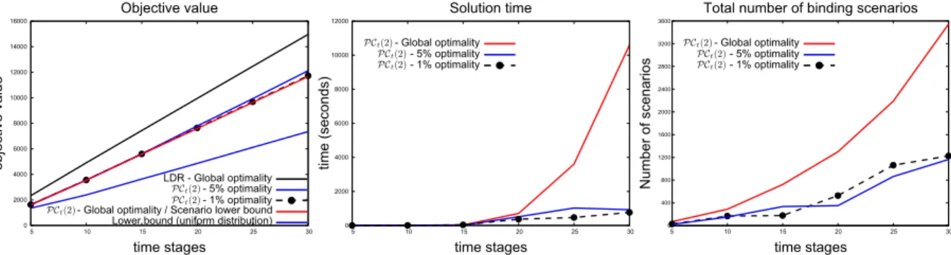
The approximations are benchmarked against the lower bounding, scenario tree problem (34) constructed using the binding scenarios from the proposed decision rules. Table 1 presents the results from this test series in terms of the average relative gap between the optimal value of the decision rule problem and the
optimal value of the lower bounding problem. The relative gap is defined as quantity (ub−lb)
2(ub+lb), where ub
and lb are the corresponding objective values for the upper and lower bounding problems. Moreover, we present the performance of the approximation when the termination criteria for the mixed-integer linear
optimization problem inStep 2of the algorithms is set to global optimality, 1% and 5% optimality gap.
We emphasize that for linear and piecewise linear decisions expressed in the form x(ξt) =x>L(ξt), the
![Table 1: Average optimality gaps from 25 randomly chosen instances for the linear decision rules (LDR), piecewise linear decision rules x(ξ t ) = x > L(ξ t ) discussed in [5, 23] and the proposed piecewise linear decision rules PC t (2) with two linear](https://thumb-us.123doks.com/thumbv2/123dok_us/433559.2550044/27.892.134.761.119.255/average-optimality-randomly-instances-decision-piecewise-discussed-piecewise.webp)