Al-Shabandar, R, Hussain, A, Liatsis, P and Keight, R
Detecting At-Risk Students with Early Interventions Using Machine Learning
Techniques
http://researchonline.ljmu.ac.uk/id/eprint/11373/
Article
LJMU has developed LJMU Research Online for users to access the research output of the
University more effectively. Copyright © and Moral Rights for the papers on this site are retained by the individual authors and/or other copyright owners. Users may download and/or print one copy of any article(s) in LJMU Research Online to facilitate their private study or for non-commercial research. You may not engage in further distribution of the material or use it for any profit-making activities or any commercial gain.
The version presented here may differ from the published version or from the version of the record. Please see the repository URL above for details on accessing the published version and note that access may require a subscription.
For more information please contact [email protected]
http://researchonline.ljmu.ac.uk/
Citation
(please note it is advisable to refer to the publisher’s version if you
intend to cite from this work)
Al-Shabandar, R, Hussain, A, Liatsis, P and Keight, R Detecting At-Risk
Students with Early Interventions Using Machine Learning Techniques.
IEEE Access. ISSN 2169-3536 (Accepted)
VOLUME XX, 2018 1
Date of publication xxxx 00, 0000, date of current version xxxx 00, 0000.
Digital Object Identifier 10.1109/ACCESS.2017.Doi Number
Detecting At-Risk Students with Early
Interventions Using Machine Learning
Techniques
Raghad Al-Shabandar 1, Abir Jaafar Hussain1, Member, IEEE, Panos Liatsis3, Senior
Member, IEEE and Robert Keight1
1Faculty of Engineering and Technology, Liverpool John Moores University, Liverpool, L33AF, UK
2Department of Electrical Engineering and Computer Science, Khalifa University, Abu Dhabi, United Arab Emirates
Corresponding author: Abir Jaafar Hussain ([email protected]).
ABSTRACT
: Massive Open Online Courses (MOOCs) have shown rapid development in recent years, allowing learners to access high-quality digital material. Because of facilitated learning and the flexibility of the teaching environment, the number of participants is rapidly growing. However, extensive research reports that the high attrition rate and lowcompletion rate are major concerns. In this paper, the early identification of students who are at risk of withdrew and failure is provided. Therefore, two models are constructed namely at-risk student model and learning achievement model. The models have the potential to detect the students who are in danger of failing and withdrawal at the early stage of the
online course. The result reveals that all classifiers gain good accuracy across both models, the highest performance yield by GBM with the value of 0.894, 0.952 for first, second model respectively, while RF yield the value of 0.866, in at-risk student framework achieved the lowest accuracy. The proposed frameworks can be used to assist instructors in delivering intensive intervention support to at-risk students.
INDEX TERMS Machine Learning; Massive Open Online Courses; Receiver Operator Characteristics; Area Under Curve.
I. INTRODUCTION
The use of Information Communication Technology (ICT) has become widespread and plays a vital role in education. ICT has contributed to the support of the academic curriculum and allows for the creation of a virtual classroom. ICT could improve student outcomes and enables instructors to aid students in solving exercises. Therefore, high-quality teaching could be delivered through virtual learning [1].
The recent boom in ICT has led to an increase in the growth of Massive Open Online Courses (MOOCs) in higher education. MOOCs provide a variety of multimedia tools to deliver an interactive learning environment. MOOCs offer valuable digital learning resources, allowing students to access information from all over the world [2].
Due to the breakdown of financial and geographical obstacles associated with the traditional teaching approach, a number of the top-ranked universities adopted online
courses as an alternative to traditional learning. With the rapid growth of online courses in higher education, low completion rates is a major issue related to MOOCs [3].
Identifying at-risk students is one of the strategies, which can be used to improve completion rates. Detecting at-risk students in a timely manner could help educators deliver instructional interventions and improve the structure of courses [4]. With a timely intervention solution, instructors can provide real-time feedback to students, and retention rates could be improved [5].
To build an accurate at-risk student prediction model, researchers investigated the reasons behind course withdrawal.This has been attributed to a number of factors.The main reason for students dropping out of online courses is the lack of motivation [6]. Researchers suggested that students’ motivational levels in online courses either decrease or increase according to social, cognitive and
2 VOLUME XX, 2018 environmental factors [7]. The motivational trajectory is an
important indicator of student dropout. Motivational trajectories can be measured by exploring changes in learner behaviour across courses [7]. Until now, most researchers did not pay attention in examining the association between motivational trajectories, student learning achievement and at-risk students in the online setting.
Predicting student retention in MOOCs can provide valuable information to help educators to early recognise at-risk students. Although a number of works were reported in the literature proposing robust learning frameworks for online courses, it is still challenging to achieve high prediction accuracy of student performance in the long term over multiple datasets [8], [9].
Two case studies are conducted in this research. The first study proposes a novel dropout predictive model, which is capable of delivering timely intervention support for at-risk students. Machine learning is employed to detect potential patterns of learner attrition from course activities and through analysing learner historical behaviour.Student engagement, in conjunction with motivational status in previous courses, were examined to evaluate their effect on students persisting with participation in the present course. In the second case study, a student performance prediction model is proposed.The model offers new insight into the key factors of learning activities and can support educators in the monitoring of student performance. Machine learning is utilized to track student performance and provide valuable information to educator to subsequent the courses according to their learning achievement. In addition ,it could help academic advisors to detect student low academic achievement and offer support for them
The remainder of this paper is organized as follows. Section II provides an overview of state-of-the-art research in the field. The methodology of the proposed approach is presented in section III, including dataset description, techniques and simulation results. The conclusions of this work and avenues for future research are described in Section IV.
II. LITERATURE REVIEW
Student withdrawal and learning achievements are a major concern in MOOCs. In this section, we provide a review of the state-of-the-art researches in the detection of at-risk students with respect to dropout and failure.
Feedforward neural networks were implemented in [10] to detect at-risk students in MOOCs, using student sentiments and clickstream as baseline features. The data was collected from 3 million student click logs in addition to 5,000 forum posts via the Coursera platform in 2014. Dealing with an imbalanced dataset was one of the main concerns in this study. This was overcome by employing Cohen's Kappa criteria instead of accuracy. The results demonstrated an accuracy of 74%, when both sets of features were employed. This reduced to 70%, when sentiment features were excluded.
In [11], at-risk students were identified by applying various machine learning algorithms, including regularized logistic regression, support vector machines, random forest, decision tree and Naïve Bayes. A set of features were captured from behavioural log data, including the number of times students visited the home page and the length of the session. The results illustrated that regularized logistic regression models achieved the highest AUC.
The ConRec Network model, a type of deep neural network, was proposed in [12]. In this work, Convolutional Neural Networks (CNN) were combined with Recurrent Neural Networks (RNN) to predict whether students are at risk of withdrawal from the online course “XuetangX” in the next ten days. Student records were structured according to a sequence of time-stamps and contained various attributes such as event time, event type and student enrolment date. The hybrid neural network model consists of two parts, namely, the lower and upper parts. In the lower part, the hidden layer of CNN was utilized to extract features automatically. In the upper part, RNN was used to make a prediction by aggregating and combining the extracted features at each time. The model was compared with various baseline methods. The results indicated similar performance across all models. The F1-score results were reported in the range of 90.74-92.48. Although there was similarity in performance, the authors argued that the ConRec Network model is more efficient than baseline methods, as it has the ability to extract the features automatically from student records without the need of feature engineering [12].
A number of features have been considered by researchers to identify the level of student learner achievement in the online setting, such as how long students interact with digital resources when students submitted assessments and the total number of attempts undertaken, educational level, geographical location and gender. In [13], Genetic Algorithms (GA) were used to optimize the feature set. The findings indicated that high ranked features are related to behavioural attributes instead of demographic features. Four classifiers were considered to predict student performance, namely decision tree, neural network, Naïve Bayes and k-nearest neighbour. Simulation results indicated that accuracy was improved by 12% when using the GA-optimized feature set. Using the decision tree with the complete feature set led to an accuracy of 83.87%, while when the GA-optimized feature set was used, accuracy jumped to 94.09% [13]. Hidden Markov models were used to measure how latent variables in conjunction with observed variables could impact student performance in virtual learning environments. A two-layer hidden Markov model (TL-HMM) was proposed in[8] to infer latent student behavioural patterns. TL-HMM differs from conventional HMM in its capacity to discover the micro-behavioural patterns of students in more detail and detect transition between latent states. For instance, when students undertake quizzes, they would tend to participate in forum discussions. The model can also learn specific transitions
3 VOLUME XX, 2018 between quiz assessment date and submission date. The
research concluded that high performing students have fewer latent behavioural states since they have sufficient knowledge, and thus, they do not need further support [8].
TABLE 1
Overview of previous research in the identification of at-risk students in MOOCs
Author Year Features Results Minaei-Bidgoli et al.,[13] 2003 Click stream features GAimproved by 12% for All classifiers.
Chaplot et al., [10] 2015 Sentiments , click stream features
Neural network attain higher performance , when using sentiment features.
He et al., [11] 2015 Click stream features
Regularized logistic regression acquired the
best AUC. Geigle et al., [8] 2017 Behavioural
attributes TL-HMM is able to infer latent behavioural patterns
Wanli et al., [12] 2018 Behavioural
attributes Deep learning is
able to extract features automatically.
III. RESEARCH METHODOLOGY
A. Data Description
Two datasets are utilised in our experiments. The first set is obtained from Harvard University and Massachusetts Institute of Technology online courses, while the second set is related to Open University online courses.
Harvard University collaborated with Massachusetts Institute of Technology (MIT) in developing online courses. The primary attribute of the Harvard dataset is the clickstream, which represents the number of events that correspond to user interaction with courseware. Qualifying events include clicking on a chapter or on forum posts and accessing the home page of videos. The user must register on each course before the actual enrolment date [14]. To complete the registration process, the user must click on five web pages.
The “Nchapters” feature is the number of chapters that learners are required to read. ”Nplay_video” represents the number of events during which the learner viewed a particular video. The “Explored” feature is a binary discretisation of exploratory learners. To be classified as an explorer, a learner must have accessed more than half of the course contents. The “Viewed” feature is also a binary feature, which is set to 1 when a student accessed the home page of assignments and related videos [15].
The date of learner registration for a specific course is recorded in the dataset in addition to the date of the learners’ last interaction with the courseware. The “LoE_DI” feature
is a demographic feature, which represents the learners’ educational level. “age “and “gender” are other types of demographic features, which are also recorded [15]. The assignment grade is an indicator attribute that represents the failure/success rate of participants. Table 2 provides a brief overview of the Harvard dataset.
TABLE 2
Harvard Dataset Overview Features Type Description
User-Id Demographic Learner identification number YOB Demographic Learner date of birth Gender Demographic Learner gender LOE Demographic Learner educational level final_cc_cname_DI Demographic Learner continent area Start_time_DI Temporal First date of learner activity last_event_DI Temporal Last date of learner activity ndays_act Temporal Number of unique days that the
learner interacted with the course Nevent Behavioural Number of click stream events nplay_video Behavioural Number of videos viewed by
learner
Nchapters Behavioural Number of chapters read by learner nforum_post Behavioural Number of forum postings by
learner
Viewed Behavioural user access to home page of quizzes
Explored Behavioural user access to home page of chapters
The second database in this study was obtained from the Open University in the UK [16]. The Open University delivers various online courses for undergraduate and postgraduate students. During 2013-2014, the Open University released a dashboard known as the Open University Learning Analytics Dataset (OULAD) Demographic, behavioural and temporal features are captured in this dataset. It includes a set of tables related to student performance, student personal information, in addition to student interaction features with online courses. The student can interact with various types of digital material, such as PDF files, access to the home and sub-pages, and taking part in quizzes [16]. There are two types of assessments, namely, the Tutor Marked Assessment (TMA) and the Computer Marked Assessment (CMA). The final average grade is computed as the weighted sum of all assessments (50%) and final exams (50%). The “Student Assessment” table involves information related to student assessment results, such as the date of the submitted assessment and the assessment mark. The assessments are mandatory in the dataset. Therefore, students are required to undertake assessments (including a final exam), if they want to remain in the course. A student will succeed in the course if s/he gains an overall grade greater than 40% [16]. Table 3 provides a brief overview of the OULAD dataset.
4 VOLUME XX, 2018 The learners Virtual Learning Environment (VLE) data
were collected on a daily basis, and feature extraction was applied. The extracted VLE features rely on clickstream features. The OULAD dataset contains eleven VLE activity types. For each student, we aggregated the number of clicks that students interacted per activity, since the first time they engaged in the course till the last day they quit the course. Twenty-two features are extracted from the VLE similarly to previous work [17]. Table 3 provides an overview of the OULAD dataset.
TABLE3
OULAD Dataset Overview
B. Course Description
In terms of the Harvard dataset, four courses are selected for analysis in this study, namely, “Introduction to Computer Science”, “Circuits and Electronics”, “Health in Numbers: Quantitative Methods in Clinical & Public Health Research” and “Human Health and Global Environmental Change”.
The “Introduction to Computer Science” course focuses on teaching students the use of computation in task solving [18]. The “Circuits and Electronics” course is an introduction to lumped circuit abstraction. The course was designed to serve undergraduate students at the Massachusetts Institute of Technology and is available online to learners worldwide [19].
“Health in Numbers: Quantitative Methods in Clinical & Public Health Research” is a health research course that was designed to teach students the use of quantitative methods in monitoring of patients’ health records. In the “Human Health and Global Environmental Change” course, students learn to
investigate how changes in the global environment could affect the health of individuals. The reason why these particular four courses were selected is that they were the only courses providing temporal information [20].
With regards to the OULAD dataset, the only available VLE data pertained to the “Social Science” course, which was launched in two semesters during the academic year 2013-2014 [16]. The courses acronyms are shown in Table 4 .
C. At-Risk Student Framework
In previous work [21], Learning Analytics (LA) tools were utilized to characterize the students’ motivational status based on Incentive Motivation Theory (IM). According to this theory, learners are classified into three categories, namely, amotivation, extrinsic, and intrinsic. Student motivation changes over time across multiple courses and could affect a student’s decision to quit the course.
Since students in the OULAD courses are required to participate in assessments, intrinsically motivated and amotivatied students cannot be evaluated for this dataset [22].Therefore, the at-risk student detection framework is only considered with the Harvard dataset, as the aim is to assess how motivation trajectories could impact at-risk students.
Learning trajectories can facilitate online course analysis by tracing student activities over time. In this study, LA is utilized in the tracking of learning trajectories across multiple courses. Figure 1 illustrates the at-risk student framework.
We propose an algorithm (Algorithm 1) to identify at-risk students in online courses, based on the course trajectories concept. Two intervals are defined in our algorithm (T1, T2). In T1, the learners who engaged only in fall course are selected
Features Description
id_student Learner identification number age_band Learner age
Gender Learner gender highest_education Learner educational level
Region Learner geographic area
studied_credits The number of credits for the module that the learner is currently involved disability Indicator of student disability num_of_prev_attempt Number of times that student undertook
the course
imd_band Socio-economic indicator measure of student economic level
leaerning activity The type and number of daily activities that the student undertakes
grades The student’s assessment marks date_registration The date of learner registration in the
course
date_unregistration The date that the learner quit the course
TABLE4
COURSE ACRONYM
Course Course Acronym Circuits and Electronics Fall Electronics Fall Circuits and Electronics Spring Electronics Spring Introduction to Computer Science and
Programming Fall
Computer Science Fall
Introduction to Computer Science and Programming Spring
Computer Science Spring
Health in Numbers: Quantitative Methods in Clinical & Public Health
Research
Health Fall
Human Health and Global Environmental Change
Health Spring
Social Science First Semester Social Science Fall Social Science Second Semester Social Science
5 VOLUME XX, 2018 while the learners who participated in both falls and spring
semester courses are considered in T2.
As suggested in [21], three categories of learners are defined, i.e., intrinsic (RL), extrinsic (CLsc, CLsn), and amotivation (Al). The assignment cutoff grade (40%) was employed for distinguishing between failing and successful extrinsic learners. Students who withdrew from a course within a period of seven days are considered amotivation students. If a student’s motivational status is amotivation during the spring semester courses, then the student can be defined as withdrawn. The algorithm makes a significant contribution by detecting patterns in student motivation trajectories. Using this approach, the proposed algorithm can facilitate course instructors in providing timely interventions to assist at-risk students.
It has been suggested that low student performance and learning achievement outcomes are important factors for students withdrawal from online courses [23]. However, in the current case study, students are defined as at risk if they withdraw from spring courses within the period of one week. This is because it is not possible to perform a reliable evaluation of student learning in such a short period.
Although intrinsically motivated students can attain learning outcomes within one week, in the Harvard dataset, it is not possible to measure student performance for such students, since relevant information, e.g., student feedback is not captured [24]. A data-driven approach should be considered when investigating the most critical factors which impact on student learning outcomes. To examine how such factors influence students who are at risk of failure, a student learning achievement model is proposed.
Let Ri Vrepresent the ith student record, given as:
Ri = < si, gi, di, ei, ci, li, wi >
D. Learning Achievement Framework
Learning achievement is considered a vital indicator of the effectiveness of the MOOCs platform [23]. A student performance predictive model is proposed to predict whether students will pass or fail in online courses. The framework aims to measure poor student performance and investigate the impact of learning activities that influence student decisions to complete a future course. This will assist instructors in drawing inferences about student performance and will offer deeper insights into the learning process. Additionally, it could
Algorithm 1 At-Risk Students
1: Let 𝑐𝑖,∈𝐶𝑝, where 𝐶𝑝is a set of courses 2: Let t ∈T where T is a set of intervals T={ 𝑇1, 𝑇2} 3: Let 𝑠𝑖,∈ 𝑆𝑣, where 𝑆𝑣, is a set of students who enrol
(𝑐𝑖)𝑇1 ∧ (𝑐𝑖)𝑇2
4: Let 𝑑𝑖,∈𝐷𝑚,where𝐷𝑚,is a set of student motivation
status where m ∈ { 𝑅𝐿, 𝐴𝑙, 𝐶𝐿𝑠𝑐 } 𝑅𝑖∈ 𝑅𝐿↔ 𝑔𝑖= 0;𝑙𝑖< 𝑑𝑖,𝑤𝑖 < 𝑒𝑖 𝑅𝑖∈ 𝐴𝑙 ↔ 𝑔𝑖= 0;𝑒𝑖− 𝑑𝑖< 8 𝑅𝑖∈ 𝐶𝐿𝑠𝑐↔ 𝑔𝑖≥ 40;𝑑𝑖≤ 𝑙𝑖 𝑅𝑖∈ 𝐶𝐿𝑠𝑛↔ 0 < 𝑔𝑖< 40;𝑑𝑖≤ 𝑙𝑖 5: ∀𝑦𝑖∈ 𝑆𝑣,: if 𝑑𝑖, at T2∈Al Then 𝑦𝑖=” withdrawal Student” Else 𝑦𝑖=” non-withdrawal Student ”
Where si - Identity of the student for the ith record
gi - Grade of the ith student record
di - Start date of associated student interaction with
course
ei - End date of associated student interaction with
course
ci - Identity of the course associated with the ith entry
li - Launch date of the course referred to by ci
wi - Wrap date of the certification issued by ci
6 VOLUME XX, 2018 support instructors in racking student progress for each tier of
learning. Hence, effective teaching can be delivered.
LA is utilized to examine the factors that affect student learning achievement using the two datasets. With LA, decision-makers would be able to acquire a more in-depth insight into the ground truth behind learner success and failure within MOOCs platforms across various courses [23].
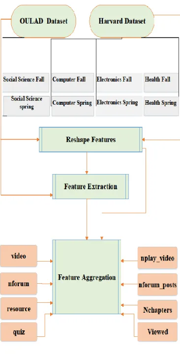
The key challenge in building a learning achievement model over two datasets is how to reshape the features. The structure of the Harvard and OULAD courses is similar to traditional courses, where the syllabus consists of a set of video lectures, pdf files and a set of multiple choice quizzes, in addition to the final exam. However, they are different with respect to data representation [24][16].
The Harvard dataset does not provide a granular record structure for student activity over time. Instead, summary values are provided, which incorporate totals, with the intermediate structure discarded. On the other hand, daily learning activities are collected in the OULAD dataset.
Clickstreams information is employed to acquire a common set of attributes across the two datasets. Specifically, the daily VLE activities are used to construct summative behavioural features across the OULAD dataset. Only four activities are considered, i.e., “nforum”, “resource”, “quiz” and “videos”. Next, the extracted features are aggregated with OULAD behavioural features these are”nfroum_posts”,“Nchapters”,”Viewed”and “nplay_vedio” Thus, similar behavioural attributes can be extracted from the two datasets.
With regards to temporal features, the number of days that learners interact with the OULAD online courses is extracted by computing the difference between the dates of student registration and deregistration from MOOCs. The same feature extraction process is performed in the Harvard dataset. Due to the weak association between learning outcomes and demographic features [25], demographic characteristics are excluded in this analysis. Figure 2 illustrates the Learning Achievement framework.
Figure 2. The proposed Learning Achievement framework. E. Data Pre-Processing
The first step in pre-processing is cleaning the data by detecting the occurrence of missing values. Several variables in the Harvard dataset have null values; examples of these include “Nevent”, “nplay_video”, “Nchapters”, “nforum_post”, “YOB”, “Gender” and “LoE_DI” attributes. The data is cleaned by removing missing values and others. In addition, student records with duplicated rows are also removed.
The Harvard dataset is non-normally distributed. In order to address this problem, transformation methods were applied. The BOX_COST transformation [26] was used to
7 VOLUME XX, 2018 transform the data distribution into normal. As seen in Table
5, the Box-Cox method transformed ten features with skewed distributions. The scaling and centring transforms were also applied , and results show that all features are centred to a mean value of 0 and scaled to a standard deviation of 1.
Data Pre-Processing is applied to the extracted behavioural features and demographic variables of the OULAD dataset, with the aim to achieve the best performance. The first step in pre-processing the data is to investigate highly correlated variables. We set a correlation cut off value of 0.8, i.e., if the correlation between two features is greater than 0.8, then these features are considered highly correlated. Highly correlated features are removed from the model, given that the problem of feature redundancy could be solved. Moreover, the occurrence of over-fitting may also be reduced. The zero and near-zero variance predictors are also investigated in this database; the features with the same values that appear frequently become zero variance predictors when the data is split into training and test. These features, which have a “near-zero-variance” are diagnosed and eliminated during the pre-processing procedure.
The Open University dataset is non-normally distributed; in order to address this problem, transformation methods are applied. Yeo-Johnson [27]is one of the data transformations methods and performs a similar function to the Box-Cox transformation, in which a continuous variable that has a raw value equal to zero is applied [27]. In our case, when a student did not participate in a particular activity, the value of the extracted features become zero. To this end, Yeo-Johnson is more useful than Box-Cox.
F. Exploratory Data Analysis (EDA)
Exploratory Data Analysis (EDA) is implemented in this study in order to gain insight into the learners’ motivational trajectories in conjunction with their dropout rate. EDA is an important step in machine learning, providing intuition about the structure and relationships within the dataset [28], [29].
With regards to the first case study, the objective of data visualization is to provide information and understanding of the type of motivational status at the first-time interval , which is more relevant to at-risk students.
Figure 3 visualizes the correlation between motivational statues and at-risk students more intuitively. It shows that learners who are intrinsically and extrinsically motivated in the fall semester courses withdraw from the spring semester course within a week. Approximately 31% of amotivation students withdrew in the subsequent course, while the proportion of withdrawal students sharply increased for the intrinsically and extrinsically motivated. It is noticeable that 84% and 77% of the intrinsically motivated and the extrinsically motivated students, respectively, dropped out in the spring course.
Principal Component Analysis (PCA) is used in the OULAD dataset to reduce redundancy due to the presence of highly correlated across the extracted features. This is only applied on the behavioural features as only learners activities are employed to track student performance[25]. To determine the number of principal components, the Kaiser method is used [30].The Kaiser approach is based on 𝜎2
to
detect the number of optimal components, and retains components that have√𝜎 > 1
[31]. Figure 4 illustrates the PCA for OULAD dataset, which exhibits low variance. The optimal number of principal components was found to be equal to 10 in this dataset. Figure 5 illustrates the results of the Kaiser method, which shows that nine components are selected as the optimal.Features Sample Skewness Estimated Lambda userid_DI 0.0135 0.70 0.1 final_cc_cname_DI -0.569 1.2 LoE_DI -0.163 0.7 YoB -1.4 2 start_time_DI -0.107 0.7 last_event_DI 0.0376 0.7 nevents 3.18 -0.1 ndays_act 1.76 0 nplay_video 6.21 0.1 nchapters 1.07 -0.4
Figure 3. Distribution of learners according to motivational status
TABLE5
8 VOLUME XX, 2018
Figure 4. PCA for the OULAD Dataset
Figure 5. Selection of principal components with the Kaiser method for the OULAD dataset
G. Dropout prediction model based on motivational status
A temporal dropout predictive model was constructed that aims to examine the influence of motivational trajectories and engagement levels on the students’ decisions to withdraw from courses. A variety of machine learning models are used, including Random Forest (RF), Feedforward Neural Network with a single hidden layer (NNET1), Multi-Layer Perceptron (NNET2) with two hidden layers, Gradient Boosting Machine (GBM) and Generalized Linear Model (GLM).
1) MODEL CONSTRUCTION AND VALIDATION
The dropout prediction model contains 4,800 records for non-withdrawal students and 6,500 records for withdrawal students. Two sets of experiments based on different sets of features were conducted in this study. Behavioural features were considered at the first and second time intervals in the first set of experiments. In the second set of experiments, only high-ranking features were selected. The original
dataset was split in half to be used as cross-validation .The cross-validation, allocate 30% for the training set and 20% for validation set . In this study, ten-fold cross-validation with five repetitions was considered. A further 50% of the data is used as an external test dataset to validate generalization errors for each model.
We propose an algorithm for early detection of at-risk students in online courses. The algorithm can be used in a classification setting, where students are classified according to their learning trajectories. It overcomes the issue of feature redundancy. Thus, the algorithm can be applied in a high dimensional dataset to enhance the efficiency and effectiveness of the predictive model.
The chi-square test is utilised to evaluate high-ranking features. If the chi-square test value is lower than a critical value (i.e., 0.05 ) then the null hypothesis is accepted, and the feature is considered as important; otherwise, the null hypothesis is rejected, and the feature is discarded. Five linear and nonlinear classifiers are employed to detect at-risk students in online courses. Two sets of features are trained and tested for each classifier. The performance of classifiers is also evaluated in the proposed framework.
Algorithm 2 At-Risk Student prediction algorithm
Input: S is a set of n samples where S={ (𝑍1,𝑦1)}), . . (𝑍𝑛,𝑦𝑛)} Z is a set of m-dimensional behavioral features where Zi= {𝑧𝑖1,𝑧𝑖2,….𝑧𝑖𝑚,}
Y is a set of target values Y = {y1, ……yn} Let H be a set of selected features
Max-iteration is the maximum number of iterations
Output: Let 𝑌∧ is set of set of predicted values where 𝑌∧= {𝑦1Λ,… 𝑦𝑛Λ}
1: for i = 1 … Max-iteration, do
2: for j=1…n ,do
3: Calculate feature weights by using Eqn. 1 end for 4: If (𝜒𝑗2 >0.05) then 𝑍𝑖 is not Important else 𝑍𝑖 is Important H = H ∪ 𝑍𝑖 end if end for
5: 𝐿𝑒𝑡 ML is set of machine learning models where ML={ NNET2, RF, Rpart, Glm, Gbm, NNET1}
6: Let P to be a set of performance matrix where P = { Acc, F1, Sens, Spec, AUC }
7: Training1 = { tr ∈ S ⇒ tr ⋉ S} 8: Training2 = { ta ∈ H ⇒ ta ⋉ S}
9: Test1 = { ts ∈ S ⇒ ts ⋉ S & ts ∉ Training1} 10: Test 2= { tn ∈ H ⇒ tn ⋉ S & tn ∉ Training2} 11: f𝐨𝐫 ∀ ML do
12: Compute 𝑌∧ for first set of features 13: E[P1] = { S: S ⇒ML(Training1, Test1)} 14: Compute 𝑌∧ for second set of features 15: E[P2] = { S: S ⇒ML(Training2, Test2)}
9 VOLUME XX, 2018
where χi2 is Chi-square calculator tests . The Niec is the
observed
frequencies of variablesZi in class c , and Εi𝑒𝑐 isthe expected frequencies for the Zi . The test compares the observed values with the expected values and determines the most relevant features as defined in Eq.(1).
𝜒𝑖2 = ∑
(𝑁𝑖𝑒𝑐− Εi𝑒𝑐)2
Εi𝑒𝑐 𝑐 ∊{0,1}
(1)
H. Learning Achievement Model
To predict whether students are at risk of failing, it is important to determine the factors that impact student learning achievement. The training dataset consists of 5000 records, which are randomly sampled from the Harvard and OULAD datasets. Only Fall courses are considered for training. The test data consists of 3000 data points, which are randomly captured from Spring courses. The Harvard and OULAD datasets are imbalanced, since 78% of the records refer to failing students (majority class), and 22% of the data relate to students succeeding (minority class). Due to the class distribution, the model may be more sensitive in predicting the majority class, thus leading to the well-known bias problem [32].
To overcome this, the training data set should be re-sampled. In this work, Synthetic Minority Over-Sampling (SMOTE) is applied. SMOTE equalizes the class proportions by generating additional minority class examples. In particular, SMOTE applies K-nearest neighbours to interpolate new instances of the minority class through an evaluation of its nearest neighbours, using a specific distance metric. Following the application of SMOTE, the balance between the two classes is considerably improved, with 57% of instances belonging to the majority class, while the remaining 42% belongs to the minority class.
In order to evaluate the learning achievement model, several quality metrics are utilised, including sensitivity, F-Measure, ROC, and AUC. Furthermore, ten-fold cross-validation is used for classification analysis, with 70% and 30% of the dataset selected for training and testing, respectively. This process is repeated 5 times.The evaluation of the predictive model is performed by using the training data with features and targets from courses that were completed and test data on the subsequent courses across the Harvard and OULAD datasets.
I. Machine Learning Algorithms Utilized in the
Experiments
RANDOM FOREST
The Random Forest model is an ensemble method that constructs multiple decision trees during the learning process, and each tree is generated using random sample vectors from the input features. The Random Forest method
can be employed for classification and regression problems [33], [34]. In terms of classification, the Random Forest method uses the voting mechanism that selects the most popular classes to classify the target. In regression, the weighted averages of trees are used in prediction [35], [33].
The Random Forest training algorithm follows the bootstrap method, given that the training dataset consists of n samples and features. Specifically, each tree is constructed by randomly selecting samples with replacement. Next, trees are created by selecting the predictor variables that give the best split. The procedure is repeated multiple times, and the tree governs the growth without pruning until the stopping criteria is achieved [36], [37].
There are two approaches which can be used to choose features in the Random Forest method, namely, Mean Decrease Impurity (MDI) and Mean Decrease Accuracy (MDA). MDI is based on decreasing the weighted impurity in a tree. Multiple nodes are created, where each node corresponds to a single feature. The Gini impurity metric for classification should be computed for each node and averaged across all trees to calculate the weighted impurity of the tree. The best features are those with the lowest impurity weight [38].
MDA relies on the Out-of-bag (OOB) error concept. As previously mentioned, trees are constructed using bootstrap samples. Some of the observation excluded from bootstrap samples and are not used in building trees [38]. The prediction error of left-out observations is called OOB error. To evaluate the importance of a particular feature, the value of this feature permutes into an OOB observation. The MDA for this feature is computed by the average difference of OOB prediction errors prior to and post permutation across all trees. Finally, feature importance is directly related to their MDA value [35], [38].
GENERALIZED LINEAR MODEL
The generalized linear model is a statistical method, which assumes that observations follow a particular distribution, namely, Average, Binomial, Poisson and Gamma. In the generalized linear model, we assume {𝑋1,…𝑋𝑛} are observations with a dependent variable 𝜂𝑖, and each linear predictor 𝜂𝑖 is generated from a particular distribution. The simple generalized linear model can be described according to the following equation [39], [40]:
𝜂𝑖= 𝛽0+ 𝛽1𝑋1+…𝛽𝑛𝑋𝑛 (2)
where Xi are the predictor variables and βi are the associated coefficients. β0 is an intercept, which can be interpreted as the mean value of 𝜂𝑖, when all predictor variables are set to zero.
There are several link functions that can be used to fit the values of variables to a linear model, such as Identity, Log, Reciprocal, Logit and Probit [41]. The basic formula of the link function is defined as [42]:
10 VOLUME XX, 2018
𝜂𝑖= 𝑔(𝜇𝑖) (3)
𝜇𝑖=𝑔−1(𝑋𝑖𝛽𝑖) (4) where 𝑔(𝜇𝑖) is the link function and 𝜂𝑖 is the linear predictor. In equations 3 and 4, the linear predictor 𝜂𝑖 equals the mean
𝜇𝑖, which is the inverse of the expected value of the predictor variables, since the data follows an exponential family density.
GRADIENT BOOSTING MACHINE
Gradientboosting is a sequence of decision trees that adopt the ensemble technique used for classification and regression tasks. The trees are trained sequentially, where early shallow trees fit the sample model of the data. Subsequent trees try to minimize the errors of previous trees. As a consequence, the final prediction model is built in the form of boosting weak classifiers into a strong classifier [43], [44].
The mean square error is used as a cost function in the Gradient boosting model. More specifically, this approach minimizes the expected values of loss for the function
Ψ(𝑌, Ϝ(𝑋𝑖)), as follows [45], [46]:
Ϝ∗(𝑋
𝑖)= arg minϜ(𝑋𝑖)𝐸𝑋,𝑌Ψ(𝑌, Ϝ(𝑋𝑖)) (5)
Friedman (2002) developed the stochastic gradient boosting the algorithm, which incorporates randomness [45]. A random subsample of the training dataset is chosen without replacement, and then, it is used to fit the base learners in each iteration of the learning process. It was concluded that randomization significantly improves the performance of the predictive model [45].
The main feature of stochastic gradient boosting is the ability to prevent overfitting in the dataset. Using a smaller subsample helps to reduce the variance of the combined trees over the iterations. Furthermore, the computational cost is smaller in stochastic gradient boosting than in gradient boosting [46], [47].
NEURAL NETWORKS
The simplest type of artificial neural networks is a single layer (perceptron) network, where the information transfers directly from the input layer to the output layer via the weight matrix. The activation function used in the single-layer perceptron network is a non-linear threshold function. The Delta rule is utilized for training the perceptron network. In the Delta rule, gradient descent is used to calculate the error between actual and predicted outputs, and the weights are adjusted so as to minimize the error [48], [49]. The activation function can be defined as follows:
𝑔(𝑥)={ 1, 𝑖𝑓 𝑍 > 𝜃 −1, 𝑜𝑡ℎ𝑒𝑟𝑤𝑖𝑠𝑒
(6) Z=𝑤1𝑥1+ ⋯ + 𝑤𝑚𝑥𝑚== ∑𝑚𝑗=1𝑤𝑚𝑥𝑚 (7)
where 𝑥𝑖 are the input values and 𝑤𝑖 are the corresponding weights. Z is the network input based on the threshold (𝜃), and the neuron is active if the values of the network input are above the threshold
.
The multilayer perceptron (MLP) is a type of feed-forward neural network that is able to learn the features of linearly inseparable data. It consists of multi-layers of units. Usually, the MLP comprises of three layers, i.e., the input layer, the output layer and at least one hidden layer. Each node of a layer is fully connected to all nodes of the previous layer through a sequence of weighted edges [50], [51].
The MLP formally consists of a number of 𝐿 layers, where each layer has a number of nodes. The collection of N units in the input layer can be described as {(𝐿𝑖)}
𝑖=1
𝑁 . {(𝐿ℎ)} ℎ=1 𝑀 is the vector representing the complete set of M units in the hidden layer h. {(𝐿𝑜)}
𝑜=1
𝑈 is the vector representing the U neurons in the output layer o. In the case of a single hidden layer, the collection of weights can be represented by two matrices { 𝑊𝑖𝑗1, 𝑊𝑘𝑗2} The weight matrix which connects the input to the hidden layer can be represented as 𝑊𝑖𝑗1, and the weight matrix that links the hidden to the output layer is
𝑊𝑘𝑗2. {(𝐵𝑖)} 𝑖=1𝐿 is the column vector of biases for layer i . Assuming the training dataset as the pair of inputs and outputs {(𝑋1,𝑌1,), … (𝑋𝑛,𝑌𝑛,)}, the input vector 𝑋𝑖, is fed to the nodes of the input layer, and then multiplied by the weight values of 𝑊𝑖𝑗1. Equation (8) shows the calculation of network inputs for unit j. The network inputs are then processed by the activation function f as follows [51]:
𝑢𝑗=∑𝑛𝑖=1𝑊𝑖𝑗1𝑋𝑖𝑛+b (8)
𝑑𝑗= 𝑓(𝑢𝑗) (9)
A similar procedure takes places for the output layer. The outputs of the hidden layer are the inputs to the output layer. The weights 𝑊𝑘𝑗2 are multiplied by the hidden layer outputs, before being fed to the transfer functions of the output neurons [51]. The weights of the MLP are adjusted using error-backpropagation [48], [49].
FEATURE SELECTION
Feature selection has been used to reduce information redundancy and improve the generalization performance of the prediction model. In terms of machine learning, feature selection considers a subset of features by eliminating features, which are redundant or irrelevant to the task at hand [52].
In the first case study, the filter approach [53], inspired by the chi-square test, is considered. The filter approach is independent of the type of classifier. Machine learning algorithms that rely on this method require less computational resources, which makes it attractive for use in large datasets. The behavioural numeric features are categorised into groups namely high,medium,low according population distribution.Table 6 illustrates the results of the chi-square test based on weight criteria. To find the most important features, we set a threshold of 0.30 according to [52]. When the weights of a feature are abovethe threshold,
11 VOLUME XX, 2018 it is considered as significant and highly correlated with the
target. The results demonstrate that the target class is highly dependent on the behavioural features in the second time interval (t2). The “ndays_act” feature acquired the largest value of 0.42 for non-at-risk students and conversely has a weak correlation with student behavioural attributes at the first time interval (t1). A good relationship between student motivational statuses at the first time interval is observed for the target at-risk students, where a value of 0.38 is obtained. This significant result indicates that student interventional motivation can be used as a robust predictor to detect students, who may be at risk of dropping out in future courses.
TABLE 6
FEATURE SELECTION RESULTS
Features Weight YOB 0.12 Gender 0. 18 LOE_DI 0.09 final_cc_cname_DI 0.11 ndays_act/
t
1 0.26 Nevent/t
1 0.25 nplay_video /t
1 0.20 Nchapters/t
1 0.23 nforum_post/t
1 0.01 Explored/t
1 0.18 motivational status/t
1 0.38 ndays_act/t
2 0.42 Nevent/t
2 0.40 nplay_video /t
2 0.39 Nchapters/t
2 0.40 nforum_post/t
2 0.17 Explored/t
2 0.29J. simulation results- Dropout Prediction Model
This section presents the simulation results for the Dropout prediction model. Student learning trajectories were tracked over fall and spring courses. The findings demonstrated that the motivational trajectory is an important factor that impacts on student completion in online courses.
The hyperparameter tuning problem was considered for both the complete set of features (all features, selected features)and the optimized sub-set in order to determine the optimal parameters for the learning algorithms in our investigations. Two methods were used to perform hyperparameter optimisation, namely, random search and grid search. The random search was applied to select the optimal number of trees and the number of samples at each split. Grid search was used to tune the number of hidden neurons and weight decay for the NNET1 and NNET2 classifiers. In this method, a combination of parameters is used to specify the optimal number of neurons and weight decay. Grid search was also used to determine the learning
rate in the GBM model, while the random search was applied to tune the number of trees. The results of hyperparameter tuning are shown in Table 7.
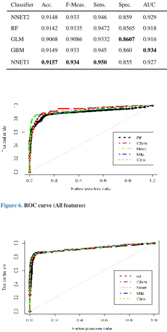
The classifiers are tested on five-step ahead prediction of at-risk students. The results over both sets of features have been compared with respect to a number of performance metrics, including accuracy, F-measure, specificity, sensitivity, and AUC. The empirical results from the second set of features (high ranking features) demonstrate slightly better performance than the first set of features (all features). As can be seen in Tables 8 and 9 for both sets of features, the NNET1 and GBM classifiers give the best accuracy, with average values of 0. 9157 and 0.894, respectively. The RF and NNET2 classifiers produce compelling results with an accuracy of 0.914 in the second set of features. Conversely, accuracy decreases by 3% and 1% in RF and GLM, over the second and first set of features, respectively, producing average values of 0.866 and 0.9068.
For both sets of features, sensitivity is seen to be slightly higher than specificity. In particular, models NNET1, NNET2 and GBM obtained sensitivities in the range of 90%-95%. Conversely, RF achieves the lowest sensitivity in the first set of features. Again, for both feature sets, GBM and GLM attained the highest specificity with average values of 0.86. The worst specificity is yielded by NNET2 across both sets of features. Figures 6 and 7 show the ROC results for both sets of features. The curves are shown to converge to roughly the same ideal result on the plot, indicating a similarity in performance across the models in both feature sets, which result in values of approximately 91% and 93%, respectively. The lowest AUC yield is obtained by RF for the first set of features.
The two feature sets were compared with respect to the learning curve. The learning curve plot provides a good indication about the early divergence between training and validation (resampling and testing), which is observed when overfitting occurs. As seen in Figures 8(a)-(b), there is overfitting across both sets of features for the RF classifiers, but in the optimized feature subset, it is not significant. With the GBM classifier, a small amount of overfitting occurs. However, its effect is not excessive in the case of high ranking features. Although the learning curves overlap in the NNET1 model, the classifier does not suffer from underfitting. Since the ROC performance is close to the ideal, the training errors decreased, when the training data was increased to 4000 samples. NNET2 is the best model, and feature selection shows a better performance. The resampling error for both sets of features is lower than the training error.
12 VOLUME XX, 2018
TABLE 7
HYPERPARAMETER TUNING PARAMETERS
Model Learning Algorithm Tuning parameters
NNET2 Backpropagation Number of units in hidden layers
First set of features (17,7), Second set of features (5,2)
weight decay
First set of features (0.01), Second set of features (0.01)
RF Number of variables
randomly sampled
First set of features (8), Second set of features (4)
Number of trees
First set of features (500), Second set of features(100) GBM AdaBoost Algorithm Number of trees
First set of features (500), Second set of features (50)
Learning rate
First set of features (0.001), Second set of features (0.01) NNET1 Backpropagation Number of units in hidden
layer
First set of features (20), Second set of features (8)
weight decay
First set of features (0.01), Second set of features (0.002)
Classifier Acc. F-Meas. Sens. Spec. AUC NNET2 0.9148 0.933 0.946 0.859 0.929 RF 0.9142 0.9335 0.9472 0.8565 0.918 GLM 0.9068 0.9086 0.9332 0.8607 0.916 GBM 0.9149 0.933 0.945 0.860 0.934 NNET1 0.9157 0.934 0.950 0.855 0.927
Figure 6. ROC curve (All features)
Figure 7. ROC curve (Optimized feature subset)
TABLE 8
CLASSIFICATION PERFORMANCE- ALL FEATURES
Classifier Acc. F-Meas. Sens. Spec. AUC NNET2 0.893 0.908 0.921 0.842 0.923 RF 0.866 0.893 0.875 0.850 0.89 GLM 0.884 0.881 0.897 0.862 0.932 GBM 0.894 0.916 0.910 0.865 0.933 NNET1 0.890 0.913 0.902 0.869 0.899 TABLE 9
13 VOLUME XX, 2018
(a) RF (All Features Set) (b) RF (Selected Features)
(c) GBM (All Features) (d) GBM (Optimized feature sub-set)
(e) NNET1 (All Features) (f) NNET1 (Optimized feature sub-set)
14 VOLUME XX, 2018
(i) GLM (All Features)
Figure 8. Comparison of learning curves for the two feature sets
K. simulation results- Learning Achievement Model
The simulation results of the learning achievement model are presented in this section. Three set of machine learning is used in this study theses including NNET1,GBM and GLM.
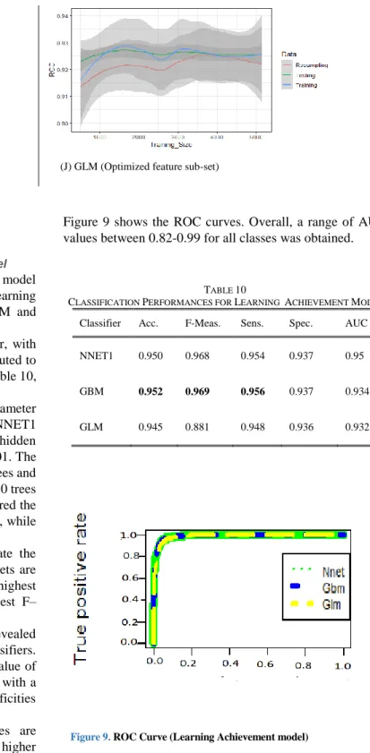
The analysis was run five times for each classifier, with average values over the five simulation rounds computed to acquire the final performance results. As shown in Table 10, accuracy is high for all classifiers.
As in the previous set of experiments, hyperparameter optimization was considered. With regards to NNET1 model, grid search suggested a hidden layer with 32 hidden units, a learning rate of 0.02, and weight decay of 0.01. The random search was used to optimize the number of trees and learning rate in GBM. The optimal parameters were 50 trees and a learning rate of 0.03. NNET1 and GBM acquired the highest accuracy, with a value of approximately 0.95, while GLM gave a slightly lower accuracy of 0.945.
The F-measure was used as a metric to evaluate the performance of the predictive model since the datasets are imbalanced. The results show that GBM achieves the highest F–measure value, whereas GLM obtained the lowest F– measure value.
The learning achievement predictive model revealed nearly ideal sensitivities and specificities for all classifiers. The best sensitivity was achieved by GBM with a value of 0.956. The lowest sensitivity was attained by GLM with a value of 0.945. All classifiers obtained good specificities values over 0.93.
Although the sensitivity and specificity values are balanced for all classifiers, the sensitivity values are higher than the corresponding specificity values. This is because the database is skewed in favour of choosing the majority class of “Failing”. In this case, predicting poor student learning achievement is more of a priority than predicting successful learners, as it could be useful for the deployment of early interventional strategies.
ROC is used in this study to choose a decision threshold value for the true and false positive rates across each class.
Figure 9 shows the ROC curves. Overall, a range of AUC values between 0.82-0.99 for all classes was obtained.
TABLE 10
CLASSIFICATION PERFORMANCES FOR LEARNING ACHIEVEMENT MODEL
Classifier Acc. F-Meas. Sens. Spec. AUC
NNET1 0.950 0.968 0.954 0.937 0.95
GBM 0.952 0.969 0.956 0.937 0.934
GLM 0.945 0.881 0.948 0.936 0.932
Figure 9. ROC Curve (Learning Achievement model)
L. DISCUSSION
A temporal predictive model was developed. In regards to feature selection, the filter approach, inspired by the chi-square test, was utilized to select the most significant features. The results show that the optimized feature sub-set includes student behavioural features in the spring semester courses, i.e., “ndays_act”, “Nevent”, “nplay_video”, and
15
“Nchapters”, in addition to the student motivational status in the fall semester courses.
Five machine learning algorithms were employed to detect at-risk students over the complete and reduced feature sets. The results of the F–Measure demonstrated that GBM and NNET1 obtain the highest performance for the full and reduced set of features, respectively, whereas RF and GLM produce the lowest performance over both sets of features. In general, the findings reveal that all classifiers demonstrated good performance.
The sensitivity values for withdrawal students are slightly higher than the specificity values for non-withdrawal students because the number of withdrawal student records is slightly higher than that of non-withdrawal student records. This could have an influence on the learning of the classifier. That is, the classifier may be biased in predicting the positive class (withdrawal student). In this study, the values of sensitivity are more important than the values of specificity, since the objective of the research is early prediction of students who may be at risk of withdrawing, so that instructors may deploy intervention strategies to support them.
The learning curve was used to investigate the overfitting problem. The findings reveal that feature selection has a significant benefit in reducing overfitting. It can be observed that any overfitting effect is not significant in the optimized feature dataset across all classifiers. With the feature selection approach, irrelevant and redundant features are eliminated. As a consequence, predictive models perform faster and more efficiently, reducing the occurrence of overfitting on the dataset and decreasing computational complexity.
The effect of behavioural engagement on student learning achievement was investigated through the tracking of student activities. The learning achievement predictive model was demonstrated in the Harvard and OULAD datasets. The input predictors consist of behavioural features, followed by the dates of student registration and deregistration from the courses. Both dataset results demonstrate that clickstream features can be reliable predictors. Indeed, this information is remarkably relevant to the prediction of student outcomes and subsequent grades for estimation of student failure. Temporal features also contain important information. For instance, the number of days that students interact with a course is highly correlated with the at-risk status.
IV. Conclusions
Two case studies were conducted in this work, with the aim of offering decision-makers the opportunity for early intervention and provision of timely assistance to students who are at risk of withdrawal and failure. In the first case study, the relationship between engagement level and motivational status with withdrawal rates was examined. In
the second case study, a learning achievement model was proposed to identify at-risk students and analyze the factors affecting student failure.
The dropout prediction model can facilitate educators in delivering early intervention support for at-risk students. The findings show that student motivation trajectories are the main reason for student withdrawal in online courses. Feature selection enhances the predictive capacity of machine learning models while reducing the associated computational costs. Furthermore, the filter method for feature selection is a promising solution for tackling the overfitting problem. The results of this study could assist educators in monitoring changes in student motivational status, thus enabling them to identify those students who require additional support.
Various factors influencing at-risk students were evaluated using the Harvard and OULAD datasets in the learning achievement model. The results in both datasets indicate that clickstream features are significant factors, which are highly correlated to student failure in online courses.
In regards to future research, we intend to consider the validation of the proposed framework with additional datasets. It will be interesting to capture online datasets from different providers, delivering courses on the same topics, to evaluate subject trends. Deep learning can also be used to automatically predict students who are in danger of dropout from courses. Deep learning can extract features from student records by inferring the sequences of temporal events across various MOOCs datasets. As such, deep convolutional neural networks can be used to track student behaviour and motivational status and discover the impact of these characteristics on at-risk students[12].
REFERENCES
[1] M. R. Ghaznavi, A. Keikha, and N.-M. Yaghoubi, “The Impact of Information and Communication Technology (ICT) on Educational Improvement,” in International Education Studies, 2011, vol. 4, no. 2, pp. 116–125.
[2] J. Sinclair and S. Kalvala, “Student engagement in massive open online courses,” Int. J. Learn. Technol., vol. 11, no. 3, p. 218, 2016.
[3] H. B. Shapiro, C. H. Lee, N. E. Wyman Roth, K. Li, M. Çetinkaya-Rundel, and D. A. Canelas, “Understanding the massive open online course (MOOC) student experience: An examination of attitudes, motivations, and barriers,” Comput. Educ., vol. 110, pp. 35–50, 2017.
[4] J.-L. Hung, M. C. Wang, S. Wang, M. Abdelrasoul, Y. Li, and W. He, “Identifying At-Risk Students for Early Interventions—A Time-Series Clustering Approach,” IEEE Trans. Emerg. Top. Comput., vol. 5, no. 1, pp. 45–55, 2017.
16
[5] T. A. R. H. A. K. R. L. A. Baker, “The Application of Gaussian Mixture Models for the Identification of At-Risk Learners in Massive Open Online Courses,” in IEEE Congress on Evolutionary Computation (CEC), 2018, pp. 1–8.
[6] M. Barak, A. Watted, and H. Haick, “Motivation to learn in massive open online courses: Examining aspects of language and social engagement,” Comput. Educ., vol. 94, pp. 49–60, 2016.
[7] J. C. Turner and H. Patrick, “How does motivation develop and why does it change? Reframing motivation research,” Educ. Psychol., vol. 43, no. 3, pp. 119–131, 2008.
[8] C. Geigle, “Modeling MOOC Student Behavior With Two-Layer Hidden Markov Models,” in In Proceedings of the Fourth (2017) ACM Conference on Learning@ Scale, 2017, vol. 9, no. 1, pp. 1–24. [9] Altair, “Improve Retail Store Performance Through
In-Store Analytics,” 2019. [Online]. Available: https://www.datawatch.com/in-action/use-cases/retail-in-store-analytics/.
[10] D. S. Chaplot, E. Rhim, and J. Kim, “Predicting student attrition in MOOCs using sentiment analysis and neural networks,” Work. 17th Int. Conf. Artif. Intell. Educ. AIED-WS 2015, vol. 1432, pp. 7–12, 2015.
[11] J. He, J. Bailey, and B. I. P. Rubinstein, “Identifying At-Risk Students in Massive Open Online Courses,” Proc. 29th AAAI Conf. Artif. Intell., pp. 1749–1755, 2015.
[12] W. Xing and D. Du, “Dropout Prediction in MOOCs: Using Deep Learning for Personalized Intervention,” J. Educ. Comput. Res.
p.0735633118757015., 2018.
[13] B. Minaei-Bidgoli, D. A. Kashy, G. Kortemeyer, and W. F. Punch, “Predicting student performance: An application of data mining methods with an educational web-based system,” Proc. - Front. Educ. Conf. FIE, vol. 1, no. December, p. T2A13-T2A18, 2003.
[14] A. D. Ho et al., “HarvardX and MITx: The First Year of Open Online Courses, Fall 2012-Summer 2013,” SSRN Electron. J., no. 1, pp. 1–33, 2014. [15] E. Summary, “HarvardX and MITx : Two Years of
Open Online Courses,” no. 10, pp. 1–37, 2015. [16] L. Analytics and C. Exchange, “OU Analyse :
Analysing at - risk students at The Open University,” in in Conference, 5th International Learning Analytics and Knowledge (LAK) (ed.), 2015, no. October 2014.
[17] R. Alshabandar, A. Hussain, R. Keight, A. Laws, and T. Baker, “The Application of Gaussian Mixture Models for the Identification of At-Risk Learners in Massive Open Online Courses,” in 2018 IEEE Congress on Evolutionary Computation,
CEC 2018 - Proceedings, 2018.
[18] J. W. D Seaton, J Reich, S Nesterko, T Mullaney, “6.00x Introduction to Computer Science and Programming MITx on edX – 2012 Fall,” New York (USA), 2014.
[19] P. F. Mitros et al., “Teaching electronic circuits online: Lessons from MITx’s 6.002x on edX,” Proc. - IEEE Int. Symp. Circuits Syst., pp. 2763– 2766, 2013.
[20] A. Reich, J., Nesterko, S., Seaton, D., Mullaney, T., Waldo, J., Chuang, I. and Ho, “PH207x: Health in Numbers & PH278x: Human Health and Global Environmental Change,” 2014.
[21] R. Al-Shabandar, A. J. Hussain, P. Liatsis, and R. Keight, “Analyzing Learners Behavior in MOOCs: An Examination of Performance and Motivation Using a Data-Driven Approach,” IEEE Access, vol. 6, pp. 73669–73685, 2018.
[22] R. Galley, “Learning Design at The Open University,” 2014.
[23] O. Zughoul et al., “Comprehensive Insights into the Criteria of Student Performance in Various
Educational Domains,” IEEE Access, vol. PP, no. November, p. 1, 2018.
[24] R. Ho, A., Chuang, I., Reich, J., Coleman, C., Whitehill, J., Northcutt, C., Williams, J., Hansen, J., Lopez, G. and Petersen, “HarvardX and MITx : Two Years of Open Online Courses Fall 2012-Summer,” in Ssrn, 2015, no. 10, pp. 1–37. [25] R. Al-shabandar, A. Hussain, A. Laws, R. Keight,
and J. Lunn, “Machine Learning Approaches to Predict Learning Outcomes in Massive Open Online Courses,” in 2017 International Joint Conference on Neural Networks (IJCNN), 2017, pp. 713–720.
[26] J. W. Osborne, “Improving your data transformations : Applying the Box-Cox
transformation,” in Practical Assessment, Research & Evaluation, 2010, p. 1–9.
[27] S. Weisberg, “Yeo-Johnson Power Transformations,” 2001, no. 2, pp. 1–4. [28] M. . Kraska, T., Talwalkar, A., Duchi, J.C.,
Griffith, R., Franklin, M.J. and Jordan, “MLbase : A Distributed Machine-learning System,” vol. 1, pp. 2–1, 2013.
[29] G. Leban, “VizRank : Data Visualization Guided by Machine,” Data Min. Knowl. Discov., pp. 119–136, 2006.
[30] D. R. Tobergte, S. Curtis, B. Lantz, D. R. Tobergte, S. Curtis, and B. Lantz, Machine Learning with R Cookbook, vol. 53, no. 9. 2013.
[31] A. Rea and W. Rea, “How Many Components should be Retained from a Multivariate Time Series PCA ?,” 2016, pp. 1–49.