An application of machine learning to statistical physics: from the phases of quantum control to satisfiability problems

(1)

OpenBU http://open.bu.edu

Theses & Dissertations Boston University Theses & Dissertations

2019

An application of machine learning

to statistical physics: from the

phases of quantum control to

satisfiability problems

https://hdl.handle.net/2144/34908

(2)

BOSTON UNIVERSITY

GRADUATE SCHOOL OF ARTS AND SCIENCES

Dissertation

AN APPLICATION OF MACHINE LEARNING TO STATISTICAL PHYSICS: FROM THE PHASES OF QUANTUM CONTROL TO

SATISFIABILITY PROBLEMS

by

ALEXANDRE GILLES RAYMOND DAY M.Sc., University of Waterloo, 2014

Submitted in partial fulfillment of the requirements for the degree of

Doctor of Philosophy 2019

(3)

(4)

Approved by First Reader Pankaj Mehta, Ph.D. Professor of Physics Second Reader Anatoli Polkovnikov, Ph.D. Professor of Physics

(5)

I have been extremely fortunate to have met curious, driven and motivated people in the course of the process leading up to this dissertation. All of this wouldn’t have been possible without my advisor and friend, Pankaj Mehta, who has, at times, given me almost absolute freedom in my intellectual endeavors and has profoundly affected the way I think. He has always been a supportive advisor and given me careful and thoughtful guidance on the problems I was working on.

My colleagues and friends, Ching-Hao, Marin, Dries, Pranay, Lei and Chris have also deeply impacted my research and I am indebted to them. Their dedication and diligence were certainly inspiring and helped me in moving forward. We have also shared innumerable laughs discussing many subjects. This has made my time at Boston University memorable and I am most thankful for having been given this opportunity.

My family has always supported me throughout this process. I am grateful to my mom and dad, for their unconditional love and support when the outcome of this work was not well defined in terms of the next step to take. My sister has also always played a great part in everything I do by giving me the motivation to explore much more than physics and maths: the world, nature and the mountains!

Finally, in the last year, the care, support and love of my girlfriend has helped me gather up the final pieces to finish this work. I am very excited about the future.

(6)

AN APPLICATION OF MACHINE LEARNING TO STATISTICAL PHYSICS: FROM THE PHASES OF QUANTUM CONTROL TO

SATISFIABILITY PROBLEMS ALEXANDRE GILLES RAYMOND DAY

Boston University, Graduate School of Arts and Sciences, 2019 Major Professor: Pankaj Mehta, Ph.D., Professor of Physics

ABSTRACT

This dissertation presents a study of machine learning methods with a focus on appli-cations to statistical and condensed matter physics, in particular the problem of quantum state preparation, spin-glass and constraint satisfiability. We will start by introducing the core principles of machine learning such as overfitting, bias-variance tradeoff and the disciplines of supervised, unsupervised and reinforcement learning. This discussion will be set in the context of recent applications of machine learning to statistical physics and condensed matter physics. We then present the problem of quantum state preparation and show how reinforcement learning along with stochastic optimization methods can be applied to identify and define phases of quantum control. Reminiscent of condensed matter physics, the underlying phases of quantum control are identified via a set of order param-eters and further detailed in terms of their universal implications for optimal quantum control. In particular, casting the optimal quantum control problem as an optimization problem, we show that it exhibits a generic glassy phase and establish a connection with the fields of spin-glass physics and constraint satisfiability problems. We then demonstrate how unsupervised learning methods can be used to obtain important information about the complexity of the phases described. We end by presenting a novel clustering framework, termed HAL for hierarchical agglomerative learning, which exploits out-of-sample accuracy estimates of machine learning classifiers to perform robust clustering of high-dimensional data. We show applications of HAL to various clustering problems.

(7)

1 Introduction 1

2 A brief overview of some important topics in machine learning 7

2.1 Intuition from Statistical Learning Theory and supervised learning . . . 7

2.1.1 The model error versus the amount of training data . . . 8

2.1.2 The model error versus the model’s complexity . . . 10

2.2 Unsupervised learning . . . 11

2.2.1 Dimensional reduction and data visualization . . . 11

2.2.2 Some of the challenges of high-dimensional data . . . 12

2.2.3 Principal component analysis (PCA) . . . 14

2.2.4 Multidimensional scaling. . . 19

2.2.5 t-SNE . . . 19

2.2.6 Clustering . . . 23

2.2.7 Practical clustering methods . . . 27

2.2.8 Clustering and Latent Variables via the Gaussian Mixture Models . 34 2.2.9 Fast density clustering . . . 39

2.2.10 Clustering in high-dimension . . . 43

2.3 Reinforcement Learning . . . 46

3 Quantum State Preparation 50 3.1 The phase diagram of quantum control . . . 50

3.2 Stochastic descent . . . 61

3.3 Algorithmic complexity and scaling of the number of local minima . . . 61

(8)

3.4 t-SNE: t-distributed stochastic neighbor embedding . . . 63

3.5 Finite-Size Scaling of the Density of States and Elementary Excitations . . 66

3.6 Finite-Size Scaling of the Order Parameters q(T) andf(T) . . . 67

3.7 The Effective Classical Spin Model . . . 67

3.7.1 Exact Coupling Strengths . . . 69

3.7.2 Better-Fidelity (Low log-Fidelity) Coupling Strengths . . . 74

3.8 Optimization as statistical physics: link to satisfiability problems . . . 80

3.8.1 Random satisfiability problems . . . 80

3.8.2 XORSAT, 3-SAT and thep-spin model . . . 81

3.9 Conclusion . . . 86

4 Hierarchical agglomerative learning 88 4.1 Related Work . . . 91

4.1.1 Out-of-sample error captures clustering performance . . . 92

4.1.2 Hierarchical agglomerative learning (HAL) - benchmarks and de-scription. . . 94

4.2 Conclusion . . . 96

5 Conclusion 100 A Supervised learning examples 101 A.0.1 Logistic regression . . . 101

A.0.2 Naive Bayes . . . 102

B Datasets 104

Bibliography 106

Curriculum Vitae 117

(9)

viii

List of Figures

Figure 1.1: The phase diagram of the two-dimensional ferromagnetic Ising model……... 2

Figure 1.2: The main elements of a reinforcement learning problem……….. 4

Figure 1.3: For every encountered state (s

i

), the agent takes an action (a

i

) based a some

policy and repeats this sequence until the termination of the episode (a finite

sequence of state-action-reward triplets)………. 5

Figure 2.1: Schematic of the typical in-sample and out-of-sample error as a function of

training set size……… 9

Figure 2.2: Bias-Variance tradeoff and model complexity……… 10

Figure 2.3: Data distributed in a three-dimensional space………. 13

Figure 2.4: Illustration of the crowding problem………... 14

Figure 2.5: PCA seeks to find the set of orthogonal directions for which those data have

the largest variance……… 15

Figure 2.6: (a) The first 2 principal components of the Ising dataset……… 16

Figure 2.7: Illustration of the t-SNE embedding………... 24

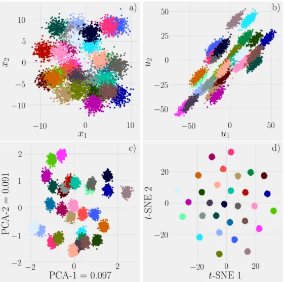
Figure 2.8: Different visualizations of a Gaussian mixture formed of K = 30 mixtures in a

D = 40 dimensional space……….. 25

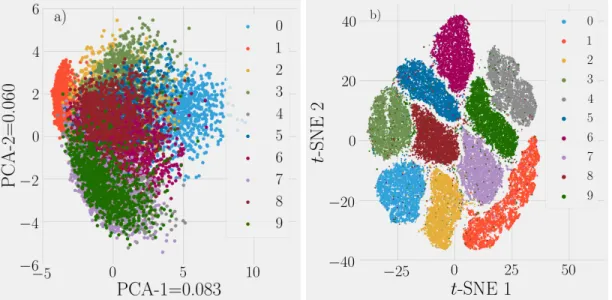
Figure 2.9: Visualization of the MNIST handwritten digits training dataset……… 26

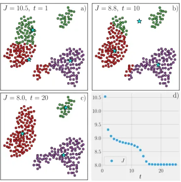
Figure 2.10: K-means with K

= 3 applied to an artificial two-dimensional dataset…….. 29

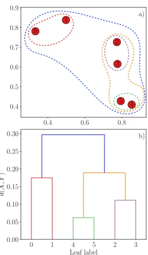
Figure 2.11: Hierarchical clustering example with single linkage……… 32

Figure 2.12: (a) Illustration of DBSCAN algorithm with

minPts

= 4, and (b) Application

of DBSCAN (

minPts

=40) to a noisy dataset with two non-convex clusters…… 34

(10)

ix

Figure 2.13: (a) Application of gaussian mixture modeling to the Ising dataset, and (b) The

gaussian mixture model can be used to compute posterior probability

(responsibilities), i.e. the probability of being in one of the phases……….. 40

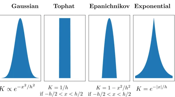
Figure 2.14: Example of some valid kernels for constructing density estimators………. 42

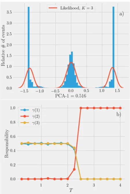
Figure 2.15: Typical shape of the log-likelihood function for the density estimator over the

test set………. 42

Figure 2.16: Noise parameter (

) which sets a threshold on what is considered true signal

versus sampling noise……… 43

Figure 2.17: Simple benchmarks for the proposed density clustering algorithm over various

low-dimensional datasets consisting of 1500 data points each……….. 44

Figure 3.1: Bang-bang protocols h(jdt) to control a quantum system with high fidelity... 51

Figure 3.2: Phase diagram for the single qubit system (L = 1)………..… 55

Figure 3.3: Preparing states in a chain of qubits……….... 56

Figure 3.4: (a)-(c) t-SNE visualization of the control landscape above the SD2 glass critical

point Tc

(2)

≈

2:3……….. 57

Figure 3.5: Normalized density of states………... 60

Figure 3.6: Average number of protocol fidelity evaluation per stochastic descent run

required to reach a local minimum of the log-fidelity landscape as a function of the

protocol duration T………. 62

Figure 3.7: The log-complexity (see Eq. (3.5)) of finding the optimal fidelity protocol... 64

Figure 3.8: Density clustering of the t-SNE embedding……… 65

Figure 3.9: Mean inter-distance for each pair of clusters found and labelled in Fig. 3.8.. 65

Figure 3.10: Distribution of the pairwise Hamming distances……….. 66

Figure 3.11: Finite-size scaling of the normalized DOS as a function of the number of

qubits L………... 67

Figure 3.12: Finite-size scaling of the normalized DOS as a function of the number of

bangs N

T

………. 68

Figure 3.13: Correlator (q(T)) scaling……… 68

43

Figure 2.16: Noise parameter (⌘) which sets a threshold on what is considered true signal versus sampling noise. In the example shown, the density estimate shown by the blue line has two modes. However one of the modes is only slightly distinguishable from the baseline. If⌘ is taken to be large enough, the smallest mode is merged with the largest.

not take into account the e↵ect of noise. Here we thus introduce a noise parameter which serves to identify wether a density maximum is true signal or is due to sampling noise. The basic idea of this parameter is shown in Fig.2.16. Using a large ⌘ parameter, implies merging nearby clusters thus leading to a coarse-graining of the clusters.

All and all, using kernel density estimates along with density graph and a noise pa-rameter, is it possible to achieve highly accurate clustering in low-dimensional spaces. Benchmarks of the method are shown in Fig.2.17.

2.2.10 Clustering in high-dimension

Clustering data in high-dimension can be very challenging. One major problem that is aggravated in high-dimensions is the accumulation of noise coming from spurious features that tends to “blur” distances [63,64, 65]. Many clustering algorithms rely on the explicit use of a similarity measure or distance metrics that weigh all features equally. For this reason, one must be careful when using an o↵-the-shelf method in high dimensions. In

(11)

x

Figure 3.15: Spatial dependence of the single-spin (`onsite magnetic field') term……… 70

Figure 3.16: Spatial dependence of the two-body interaction term………... 70

Figure 3.17: Decay of the two-body interaction terms J

ij along the anti-diagonal……… 71

Figure 3.18: Non-locality of the three-body interaction term……… 71

Figure 3.19: Left: average difference between the spectrum of the truncated effective

models and the exact fidelity spectrum as a function of the protocol duration

T.

Right: Frustration order parameter for the truncated effective models as a function

of the protocol duration T……….. 75

Figure 3.20:

R

2

of model performance vs. the protocol duration

T

for the three model

classes considered for Lasso (left) and Ridge regression (right)………. 77

Figure 3.21: Spatial dependence of the single-spin (‘onsite magnetic field’) term…..…. 78

Figure 3.22: Spatial dependence of the two-body interaction term………... 79

Figure 3.23: Non-locality of the tree-body term……… 79

Figure 3.24: Example of a XORSAT formula which is equivalent to a binary system of

linear equations……….. 81

Figure 3.25: Generic phase diagram of random satisfiability problems……… 82

Figure 3.26: Truth table for the logical XOR and AND……… 83

Figure 3.27: Clustering of the solutions for 3-XORSAT………... 84

Figure 3.28: Clustering of the solutions for 3-SAT………... 86

Figure 4.1: Validating clustering : clustering assignments can be validated by training an

expressive classifier on the clustering assignments………... 90

Figure 4.2: Out-of-sample accuracy vs. the

F-measure (comparison to ground-truth) for

various clustering algorithms………. 94

Figure 4.3: Out-of-sample error vs. the label corruption level

p (see text) for a binary

classification problem for a mixture of 2 gaussians in two dimensions………… 95

(12)

xi

Figure 4.5: Coarse-graining procedure based on out-of-sample accuracy……… 97

Figure 4.6: Normalized mutual information (NMI) as a function of the desired

out-of-sample accuracy………. 98

Figure 4.7: The hierarchical model produced by HAL can be inspected through an

interactive Dashboard……… 99

Figure A.1: Fitting a mixture of two gaussians in two dimension………... 103

Figure B.1: Sampled images from the MNIST dataset……… 105

Figure B.2: Sampled configurations from the Ising dataset (40

x

40 system)…………. 105

(13)

xii

List of Publications Contributing to this Thesis

1. Alexandre GR Day, Marin Bukov, Phillip Weinberg, Pankaj Mehta, Dries Sels

The Glassy Phase of Quantum Optimal Control

To appear in Physical Review Letters,arXiv 1803.10856

2. Marin Bukov, Alexandre GR Day, Dries Sels, Phillip Weinberg, Anatoli Polkovnikov, Pankaj Mehta

Reinforcement learning in di↵erent phases of quantum control

Physical Review X 8 (3), 031086

3. Marin Bukov, Alexandre GR Day, Phillip Weinberg, Anatoli Polkovnikov, Pankaj Mehta, Dries Sels

Broken symmetry in a two-qubit quantum control landscape

Physical Review A 97 (5), 052114

4. Pankaj Mehta, Marin Bukov, Ching-Hao Wang, Alexandre GR Day, Clint Richard-son, Charles K Fisher, David J Schwab A high-bias, low-variance introduction to machine learning for physicists

arXiv 1803.08823

(14)

xiii

List of Packages contributing to this Thesis

1. Fast density clustering (FDC):

https://github.com/alexandreday/fast density clustering

A novel robust and fast density clustering for low-dimensional data

2. Quantum state preparation optimization (Optimize QSP):

https://github.com/alexandreday/Optimize QSP

Optimization methods for quantum state preparation (reinforcement learning, stochas-tic descent and simulated annealing)

3. t-SNE visual:

https://github.com/alexandreday/tsne visual A Python wrapper for running t-SNE

4. Hierarchical agglomerative learning:

https://pypi.org/project/hal-x/

HAL: a package for clustering high-dimensional data and more

(15)

Chapter 1

Introduction

The past decade or so has seen a rapidly mounting interest for machine learning applications in many disciplines of science, from computational biology to astronomy and condensed matter physics [1, 2, 3]. This is largely due to a democratization of high performance-computing infrastructures and librairies along with an excitement around the promises of deep learning to achieve general artificial intelligence, help solve difficult problems of sciences [4] and enable new technologies such as self-driving vehicles [5], biometrics [6] and targeted health-care [7,8] to name a few. Succinctly, machine learning is a set of statistical and algorithmic tools designed to have a computer “learn” structure and predict from data. Learning, in the context of machine learning, generally means to be able to generalize (or extrapolate) from observations as oppose to learning by heart. The process of learning to generalize is usually referred to as the training phase.

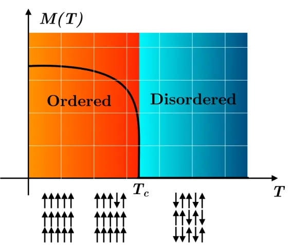
Common applications of machine learning include regression and classification, where a machine learning model is given a set of observations and is trained to predict a scalar (or a vector ∈Rn) or a discrete category respectively associated with those observations. A recent application [9] of regression machine learning in the context of condensed matter physics has been to predict the critical temperature of a superconducting material given information such as the applied pressure and the material crystal structure and chemical composition. Machine learning classification methods on the other hand have been applied to predict phases of various quantum and classical statistical physics models [3, 10] given the configuration of the degrees of freedom (see Fig.1.1). These applications are examples of supervised learning, which we will discuss in greater details in chapter2.

(16)

2

T

M(T)

T

c

Ordered

Disordered

Figure 1.1: The phase diagram of the two-dimensional ferromagnetic Ising model. The magnetization order parameter (M(T)) is plotted versus the temperature. At high-temperatures (T Tc ∼ J), the model is disordered: the typical spin configurations carry no magnetization and M(T) = 0. At low-temperature, the system exhibits a spon-taneous symmetry breaking of the Z2 symmetry and becomes ordered: the typical spin

configurations are configurations where almost all spins are aligned (M(T) _{≈ ±}1). The system undergoes a phase transition precisely at Tc. Machine learning classifiers can be trained in order to distinguish between the disordered and the ordered phases of such mod-els [3, 4]. Using unsupervised learning methods, it is also possible to identify phases by identifying clusters in the phase space of configurations (as we will discuss in chapter 2 -see also Fig. 2.13 for instance).

(17)

Reinforcement learning Recently, reinforcement learning (see Fig.1.2) has been shown to outperform humans or previous programs at various games such at Go and chess [11,

12, 13,14]. In reinforcement learning, an “agent” (i.e. an adaptive computer program) is set out to accomplish a task by performing a series of actions and is given a reward for completing this task. For instance, this task could be to win at chess [14] or to control a set of laser intensities in order to prepare a Bose-Einstein condensate [15].

Reinforcement learning has four main components: apolicy, areward, avalue function and optionally, a model [16]. The agent performs a series of actions according to a policy, which is a mapping of states to actions (see Fig.1.3). The policy followed is updated in a way to eventually maximize the rewards obtained. In order to do so, the reinforcement learning agent tries to balance theexploration of new options (previously unexplored states or/and actions) and the exploitation of its current knowledge (memory of previous actions and rewards). This is known as theexploration versusexploitation dilemma which is central to reinforcement learning. Methods that only exploit current knowledge, for instance gradient information, are said to be greedy.

The current knowledge of which states have a high value in terms of future rewards is encoded in the value function. The value function can simply be a look-up table or in more complicates cases, such as when the state space is very large, a regressor model (c.g. a neural network regressor). Finally, it is often useful to model the environment, that is, construct a model of state-action transitions generated by the environment. This is because given a state and an action taken by the agent, the subsequent state is not always known nor deterministic. Modeling the environment is useful for planning next moves and computing expected rewards [16].

Quantum state preparation Shifting our focus to quantum computing and condensed matter physics, a central problem there has been the one of preparing quantum states rapidly and reliably. Quantum state preparation is vital to many fields such nuclear mag-netic resonance experiments [17] and cold atomic systems [18,15] to trapped ions [19,20,

(18)

4

RL

Agent

Action

Environment

Reward

⇡

t

<latexit sha1_base64="2l9g2BMM56/YhZIoOzClIUbp1zk=">AAAB7HicbVBNS8NAEJ3Ur1q/qh69LBbBU0lEqMeiF48VTFtoQ9lsN+3SzSbsToQS+hu8eFDEqz/Im//GbZuDtj4YeLw3w8y8MJXCoOt+O6WNza3tnfJuZW//4PCoenzSNkmmGfdZIhPdDanhUijuo0DJu6nmNA4l74STu7nfeeLaiEQ94jTlQUxHSkSCUbSS30/FAAfVmlt3FyDrxCtIDQq0BtWv/jBhWcwVMkmN6XluikFONQom+azSzwxPKZvQEe9ZqmjMTZAvjp2RC6sMSZRoWwrJQv09kdPYmGkc2s6Y4tisenPxP6+XYXQT5EKlGXLFlouiTBJMyPxzMhSaM5RTSyjTwt5K2JhqytDmU7EheKsvr5P2Vd1z697Dda15W8RRhjM4h0vwoAFNuIcW+MBAwDO8wpujnBfn3flYtpacYuYU/sD5/AHcM460</latexit><latexit sha1_base64="2l9g2BMM56/YhZIoOzClIUbp1zk=">AAAB7HicbVBNS8NAEJ3Ur1q/qh69LBbBU0lEqMeiF48VTFtoQ9lsN+3SzSbsToQS+hu8eFDEqz/Im//GbZuDtj4YeLw3w8y8MJXCoOt+O6WNza3tnfJuZW//4PCoenzSNkmmGfdZIhPdDanhUijuo0DJu6nmNA4l74STu7nfeeLaiEQ94jTlQUxHSkSCUbSS30/FAAfVmlt3FyDrxCtIDQq0BtWv/jBhWcwVMkmN6XluikFONQom+azSzwxPKZvQEe9ZqmjMTZAvjp2RC6sMSZRoWwrJQv09kdPYmGkc2s6Y4tisenPxP6+XYXQT5EKlGXLFlouiTBJMyPxzMhSaM5RTSyjTwt5K2JhqytDmU7EheKsvr5P2Vd1z697Dda15W8RRhjM4h0vwoAFNuIcW+MBAwDO8wpujnBfn3flYtpacYuYU/sD5/AHcM460</latexit><latexit sha1_base64="2l9g2BMM56/YhZIoOzClIUbp1zk=">AAAB7HicbVBNS8NAEJ3Ur1q/qh69LBbBU0lEqMeiF48VTFtoQ9lsN+3SzSbsToQS+hu8eFDEqz/Im//GbZuDtj4YeLw3w8y8MJXCoOt+O6WNza3tnfJuZW//4PCoenzSNkmmGfdZIhPdDanhUijuo0DJu6nmNA4l74STu7nfeeLaiEQ94jTlQUxHSkSCUbSS30/FAAfVmlt3FyDrxCtIDQq0BtWv/jBhWcwVMkmN6XluikFONQom+azSzwxPKZvQEe9ZqmjMTZAvjp2RC6sMSZRoWwrJQv09kdPYmGkc2s6Y4tisenPxP6+XYXQT5EKlGXLFlouiTBJMyPxzMhSaM5RTSyjTwt5K2JhqytDmU7EheKsvr5P2Vd1z697Dda15W8RRhjM4h0vwoAFNuIcW+MBAwDO8wpujnBfn3flYtpacYuYU/sD5/AHcM460</latexit><latexit sha1_base64="2l9g2BMM56/YhZIoOzClIUbp1zk=">AAAB7HicbVBNS8NAEJ3Ur1q/qh69LBbBU0lEqMeiF48VTFtoQ9lsN+3SzSbsToQS+hu8eFDEqz/Im//GbZuDtj4YeLw3w8y8MJXCoOt+O6WNza3tnfJuZW//4PCoenzSNkmmGfdZIhPdDanhUijuo0DJu6nmNA4l74STu7nfeeLaiEQ94jTlQUxHSkSCUbSS30/FAAfVmlt3FyDrxCtIDQq0BtWv/jBhWcwVMkmN6XluikFONQom+azSzwxPKZvQEe9ZqmjMTZAvjp2RC6sMSZRoWwrJQv09kdPYmGkc2s6Y4tisenPxP6+XYXQT5EKlGXLFlouiTBJMyPxzMhSaM5RTSyjTwt5K2JhqytDmU7EheKsvr5P2Vd1z697Dda15W8RRhjM4h0vwoAFNuIcW+MBAwDO8wpujnBfn3flYtpacYuYU/sD5/AHcM460</latexit>

New state

s

t

+1

<latexit sha1_base64="ScCu8WZixoFvlWxDlnIdRy5VZ8I=">AAAB7nicbVBNS8NAEJ3Ur1q/qh69LBZBEEoigh6LXjxWsB/QhrLZbtqlm03YnQgl9Ed48aCIV3+PN/+NmzYHbX0w8Hhvhpl5QSKFQdf9dkpr6xubW+Xtys7u3v5B9fCobeJUM95isYx1N6CGS6F4CwVK3k00p1EgeSeY3OV+54lrI2L1iNOE+xEdKREKRtFKHTPI8MKbDao1t+7OQVaJV5AaFGgOql/9YczSiCtkkhrT89wE/YxqFEzyWaWfGp5QNqEj3rNU0YgbP5ufOyNnVhmSMNa2FJK5+nsio5Ex0yiwnRHFsVn2cvE/r5dieONnQiUpcsUWi8JUEoxJ/jsZCs0ZyqkllGlhbyVsTDVlaBOq2BC85ZdXSfuy7rl17+Gq1rgt4ijDCZzCOXhwDQ24hya0gMEEnuEV3pzEeXHenY9Fa8kpZo7hD5zPHwfej1o=</latexit><latexit sha1_base64="ScCu8WZixoFvlWxDlnIdRy5VZ8I=">AAAB7nicbVBNS8NAEJ3Ur1q/qh69LBZBEEoigh6LXjxWsB/QhrLZbtqlm03YnQgl9Ed48aCIV3+PN/+NmzYHbX0w8Hhvhpl5QSKFQdf9dkpr6xubW+Xtys7u3v5B9fCobeJUM95isYx1N6CGS6F4CwVK3k00p1EgeSeY3OV+54lrI2L1iNOE+xEdKREKRtFKHTPI8MKbDao1t+7OQVaJV5AaFGgOql/9YczSiCtkkhrT89wE/YxqFEzyWaWfGp5QNqEj3rNU0YgbP5ufOyNnVhmSMNa2FJK5+nsio5Ex0yiwnRHFsVn2cvE/r5dieONnQiUpcsUWi8JUEoxJ/jsZCs0ZyqkllGlhbyVsTDVlaBOq2BC85ZdXSfuy7rl17+Gq1rgt4ijDCZzCOXhwDQ24hya0gMEEnuEV3pzEeXHenY9Fa8kpZo7hD5zPHwfej1o=</latexit><latexit sha1_base64="ScCu8WZixoFvlWxDlnIdRy5VZ8I=">AAAB7nicbVBNS8NAEJ3Ur1q/qh69LBZBEEoigh6LXjxWsB/QhrLZbtqlm03YnQgl9Ed48aCIV3+PN/+NmzYHbX0w8Hhvhpl5QSKFQdf9dkpr6xubW+Xtys7u3v5B9fCobeJUM95isYx1N6CGS6F4CwVK3k00p1EgeSeY3OV+54lrI2L1iNOE+xEdKREKRtFKHTPI8MKbDao1t+7OQVaJV5AaFGgOql/9YczSiCtkkhrT89wE/YxqFEzyWaWfGp5QNqEj3rNU0YgbP5ufOyNnVhmSMNa2FJK5+nsio5Ex0yiwnRHFsVn2cvE/r5dieONnQiUpcsUWi8JUEoxJ/jsZCs0ZyqkllGlhbyVsTDVlaBOq2BC85ZdXSfuy7rl17+Gq1rgt4ijDCZzCOXhwDQ24hya0gMEEnuEV3pzEeXHenY9Fa8kpZo7hD5zPHwfej1o=</latexit><latexit sha1_base64="ScCu8WZixoFvlWxDlnIdRy5VZ8I=">AAAB7nicbVBNS8NAEJ3Ur1q/qh69LBZBEEoigh6LXjxWsB/QhrLZbtqlm03YnQgl9Ed48aCIV3+PN/+NmzYHbX0w8Hhvhpl5QSKFQdf9dkpr6xubW+Xtys7u3v5B9fCobeJUM95isYx1N6CGS6F4CwVK3k00p1EgeSeY3OV+54lrI2L1iNOE+xEdKREKRtFKHTPI8MKbDao1t+7OQVaJV5AaFGgOql/9YczSiCtkkhrT89wE/YxqFEzyWaWfGp5QNqEj3rNU0YgbP5ufOyNnVhmSMNa2FJK5+nsio5Ex0yiwnRHFsVn2cvE/r5dieONnQiUpcsUWi8JUEoxJ/jsZCs0ZyqkllGlhbyVsTDVlaBOq2BC85ZdXSfuy7rl17+Gq1rgt4ijDCZzCOXhwDQ24hya0gMEEnuEV3pzEeXHenY9Fa8kpZo7hD5zPHwfej1o=</latexit>

r

<latexit sha1_base64="dvVlgasRhCqCYveGT7iPGkroPTQ=">AAAB7HicbVBNS8NAEJ3Ur1q/qh69LBbBU0lEqMeiF48VTFtoQ9lsN+3SzSbsToQS+hu8eFDEqz/Im//GbZuDtj4YeLw3w8y8MJXCoOt+O6WNza3tnfJuZW//4PCoenzSNkmmGfdZIhPdDanhUijuo0DJu6nmNA4l74STu7nfeeLaiEQ94jTlQUxHSkSCUbSSrwc5zgbVmlt3FyDrxCtIDQq0BtWv/jBhWcwVMkmN6XluikFONQom+azSzwxPKZvQEe9ZqmjMTZAvjp2RC6sMSZRoWwrJQv09kdPYmGkc2s6Y4tisenPxP6+XYXQT5EKlGXLFlouiTBJMyPxzMhSaM5RTSyjTwt5K2JhqytDmU7EheKsvr5P2Vd1z697Dda15W8RRhjM4h0vwoAFNuIcW+MBAwDO8wpujnBfn3flYtpacYuYU/sD5/AEs9I7p</latexit><latexit sha1_base64="dvVlgasRhCqCYveGT7iPGkroPTQ=">AAAB7HicbVBNS8NAEJ3Ur1q/qh69LBbBU0lEqMeiF48VTFtoQ9lsN+3SzSbsToQS+hu8eFDEqz/Im//GbZuDtj4YeLw3w8y8MJXCoOt+O6WNza3tnfJuZW//4PCoenzSNkmmGfdZIhPdDanhUijuo0DJu6nmNA4l74STu7nfeeLaiEQ94jTlQUxHSkSCUbSSrwc5zgbVmlt3FyDrxCtIDQq0BtWv/jBhWcwVMkmN6XluikFONQom+azSzwxPKZvQEe9ZqmjMTZAvjp2RC6sMSZRoWwrJQv09kdPYmGkc2s6Y4tisenPxP6+XYXQT5EKlGXLFlouiTBJMyPxzMhSaM5RTSyjTwt5K2JhqytDmU7EheKsvr5P2Vd1z697Dda15W8RRhjM4h0vwoAFNuIcW+MBAwDO8wpujnBfn3flYtpacYuYU/sD5/AEs9I7p</latexit><latexit sha1_base64="dvVlgasRhCqCYveGT7iPGkroPTQ=">AAAB7HicbVBNS8NAEJ3Ur1q/qh69LBbBU0lEqMeiF48VTFtoQ9lsN+3SzSbsToQS+hu8eFDEqz/Im//GbZuDtj4YeLw3w8y8MJXCoOt+O6WNza3tnfJuZW//4PCoenzSNkmmGfdZIhPdDanhUijuo0DJu6nmNA4l74STu7nfeeLaiEQ94jTlQUxHSkSCUbSSrwc5zgbVmlt3FyDrxCtIDQq0BtWv/jBhWcwVMkmN6XluikFONQom+azSzwxPKZvQEe9ZqmjMTZAvjp2RC6sMSZRoWwrJQv09kdPYmGkc2s6Y4tisenPxP6+XYXQT5EKlGXLFlouiTBJMyPxzMhSaM5RTSyjTwt5K2JhqytDmU7EheKsvr5P2Vd1z697Dda15W8RRhjM4h0vwoAFNuIcW+MBAwDO8wpujnBfn3flYtpacYuYU/sD5/AEs9I7p</latexit><latexit sha1_base64="dvVlgasRhCqCYveGT7iPGkroPTQ=">AAAB7HicbVBNS8NAEJ3Ur1q/qh69LBbBU0lEqMeiF48VTFtoQ9lsN+3SzSbsToQS+hu8eFDEqz/Im//GbZuDtj4YeLw3w8y8MJXCoOt+O6WNza3tnfJuZW//4PCoenzSNkmmGfdZIhPdDanhUijuo0DJu6nmNA4l74STu7nfeeLaiEQ94jTlQUxHSkSCUbSSrwc5zgbVmlt3FyDrxCtIDQq0BtWv/jBhWcwVMkmN6XluikFONQom+azSzwxPKZvQEe9ZqmjMTZAvjp2RC6sMSZRoWwrJQv09kdPYmGkc2s6Y4tisenPxP6+XYXQT5EKlGXLFlouiTBJMyPxzMhSaM5RTSyjTwt5K2JhqytDmU7EheKsvr5P2Vd1z697Dda15W8RRhjM4h0vwoAFNuIcW+MBAwDO8wpujnBfn3flYtpacYuYU/sD5/AEs9I7p</latexit>

t

s

<latexit sha1_base64="MNjBNCuTGhMk5MW7hN8i+27I1oQ=">AAAB7HicbVBNS8NAEJ3Ur1q/qh69LBbBU0lEqMeiF48VTFtoQ9lsN+3SzSbsToQS+hu8eFDEqz/Im//GbZuDtj4YeLw3w8y8MJXCoOt+O6WNza3tnfJuZW//4PCoenzSNkmmGfdZIhPdDanhUijuo0DJu6nmNA4l74STu7nfeeLaiEQ94jTlQUxHSkSCUbSSbwY5zgbVmlt3FyDrxCtIDQq0BtWv/jBhWcwVMkmN6XluikFONQom+azSzwxPKZvQEe9ZqmjMTZAvjp2RC6sMSZRoWwrJQv09kdPYmGkc2s6Y4tisenPxP6+XYXQT5EKlGXLFlouiTBJMyPxzMhSaM5RTSyjTwt5K2JhqytDmU7EheKsvr5P2Vd1z697Dda15W8RRhjM4h0vwoAFNuIcW+MBAwDO8wpujnBfn3flYtpacYuYU/sD5/AEufI7q</latexit><latexit sha1_base64="MNjBNCuTGhMk5MW7hN8i+27I1oQ=">AAAB7HicbVBNS8NAEJ3Ur1q/qh69LBbBU0lEqMeiF48VTFtoQ9lsN+3SzSbsToQS+hu8eFDEqz/Im//GbZuDtj4YeLw3w8y8MJXCoOt+O6WNza3tnfJuZW//4PCoenzSNkmmGfdZIhPdDanhUijuo0DJu6nmNA4l74STu7nfeeLaiEQ94jTlQUxHSkSCUbSSbwY5zgbVmlt3FyDrxCtIDQq0BtWv/jBhWcwVMkmN6XluikFONQom+azSzwxPKZvQEe9ZqmjMTZAvjp2RC6sMSZRoWwrJQv09kdPYmGkc2s6Y4tisenPxP6+XYXQT5EKlGXLFlouiTBJMyPxzMhSaM5RTSyjTwt5K2JhqytDmU7EheKsvr5P2Vd1z697Dda15W8RRhjM4h0vwoAFNuIcW+MBAwDO8wpujnBfn3flYtpacYuYU/sD5/AEufI7q</latexit><latexit sha1_base64="MNjBNCuTGhMk5MW7hN8i+27I1oQ=">AAAB7HicbVBNS8NAEJ3Ur1q/qh69LBbBU0lEqMeiF48VTFtoQ9lsN+3SzSbsToQS+hu8eFDEqz/Im//GbZuDtj4YeLw3w8y8MJXCoOt+O6WNza3tnfJuZW//4PCoenzSNkmmGfdZIhPdDanhUijuo0DJu6nmNA4l74STu7nfeeLaiEQ94jTlQUxHSkSCUbSSbwY5zgbVmlt3FyDrxCtIDQq0BtWv/jBhWcwVMkmN6XluikFONQom+azSzwxPKZvQEe9ZqmjMTZAvjp2RC6sMSZRoWwrJQv09kdPYmGkc2s6Y4tisenPxP6+XYXQT5EKlGXLFlouiTBJMyPxzMhSaM5RTSyjTwt5K2JhqytDmU7EheKsvr5P2Vd1z697Dda15W8RRhjM4h0vwoAFNuIcW+MBAwDO8wpujnBfn3flYtpacYuYU/sD5/AEufI7q</latexit><latexit sha1_base64="MNjBNCuTGhMk5MW7hN8i+27I1oQ=">AAAB7HicbVBNS8NAEJ3Ur1q/qh69LBbBU0lEqMeiF48VTFtoQ9lsN+3SzSbsToQS+hu8eFDEqz/Im//GbZuDtj4YeLw3w8y8MJXCoOt+O6WNza3tnfJuZW//4PCoenzSNkmmGfdZIhPdDanhUijuo0DJu6nmNA4l74STu7nfeeLaiEQ94jTlQUxHSkSCUbSSbwY5zgbVmlt3FyDrxCtIDQq0BtWv/jBhWcwVMkmN6XluikFONQom+azSzwxPKZvQEe9ZqmjMTZAvjp2RC6sMSZRoWwrJQv09kdPYmGkc2s6Y4tisenPxP6+XYXQT5EKlGXLFlouiTBJMyPxzMhSaM5RTSyjTwt5K2JhqytDmU7EheKsvr5P2Vd1z697Dda15W8RRhjM4h0vwoAFNuIcW+MBAwDO8wpujnBfn3flYtpacYuYU/sD5/AEufI7q</latexit>

t

a

<latexit sha1_base64="7b0A7jcxySFSwS6bsYNt+eTwSsk=">AAAB7HicbVBNS8NAEJ3Ur1q/qh69LBbBU0lEqMeiF48VTFtoQ9lsN+3SzSbsToQS+hu8eFDEqz/Im//GbZuDtj4YeLw3w8y8MJXCoOt+O6WNza3tnfJuZW//4PCoenzSNkmmGfdZIhPdDanhUijuo0DJu6nmNA4l74STu7nfeeLaiEQ94jTlQUxHSkSCUbSSTwc5zgbVmlt3FyDrxCtIDQq0BtWv/jBhWcwVMkmN6XluikFONQom+azSzwxPKZvQEe9ZqmjMTZAvjp2RC6sMSZRoWwrJQv09kdPYmGkc2s6Y4tisenPxP6+XYXQT5EKlGXLFlouiTBJMyPxzMhSaM5RTSyjTwt5K2JhqytDmU7EheKsvr5P2Vd1z697Dda15W8RRhjM4h0vwoAFNuIcW+MBAwDO8wpujnBfn3flYtpacYuYU/sD5/AES7I7Y</latexit><latexit sha1_base64="7b0A7jcxySFSwS6bsYNt+eTwSsk=">AAAB7HicbVBNS8NAEJ3Ur1q/qh69LBbBU0lEqMeiF48VTFtoQ9lsN+3SzSbsToQS+hu8eFDEqz/Im//GbZuDtj4YeLw3w8y8MJXCoOt+O6WNza3tnfJuZW//4PCoenzSNkmmGfdZIhPdDanhUijuo0DJu6nmNA4l74STu7nfeeLaiEQ94jTlQUxHSkSCUbSSTwc5zgbVmlt3FyDrxCtIDQq0BtWv/jBhWcwVMkmN6XluikFONQom+azSzwxPKZvQEe9ZqmjMTZAvjp2RC6sMSZRoWwrJQv09kdPYmGkc2s6Y4tisenPxP6+XYXQT5EKlGXLFlouiTBJMyPxzMhSaM5RTSyjTwt5K2JhqytDmU7EheKsvr5P2Vd1z697Dda15W8RRhjM4h0vwoAFNuIcW+MBAwDO8wpujnBfn3flYtpacYuYU/sD5/AES7I7Y</latexit><latexit sha1_base64="7b0A7jcxySFSwS6bsYNt+eTwSsk=">AAAB7HicbVBNS8NAEJ3Ur1q/qh69LBbBU0lEqMeiF48VTFtoQ9lsN+3SzSbsToQS+hu8eFDEqz/Im//GbZuDtj4YeLw3w8y8MJXCoOt+O6WNza3tnfJuZW//4PCoenzSNkmmGfdZIhPdDanhUijuo0DJu6nmNA4l74STu7nfeeLaiEQ94jTlQUxHSkSCUbSSTwc5zgbVmlt3FyDrxCtIDQq0BtWv/jBhWcwVMkmN6XluikFONQom+azSzwxPKZvQEe9ZqmjMTZAvjp2RC6sMSZRoWwrJQv09kdPYmGkc2s6Y4tisenPxP6+XYXQT5EKlGXLFlouiTBJMyPxzMhSaM5RTSyjTwt5K2JhqytDmU7EheKsvr5P2Vd1z697Dda15W8RRhjM4h0vwoAFNuIcW+MBAwDO8wpujnBfn3flYtpacYuYU/sD5/AES7I7Y</latexit><latexit sha1_base64="7b0A7jcxySFSwS6bsYNt+eTwSsk=">AAAB7HicbVBNS8NAEJ3Ur1q/qh69LBbBU0lEqMeiF48VTFtoQ9lsN+3SzSbsToQS+hu8eFDEqz/Im//GbZuDtj4YeLw3w8y8MJXCoOt+O6WNza3tnfJuZW//4PCoenzSNkmmGfdZIhPdDanhUijuo0DJu6nmNA4l74STu7nfeeLaiEQ94jTlQUxHSkSCUbSSTwc5zgbVmlt3FyDrxCtIDQq0BtWv/jBhWcwVMkmN6XluikFONQom+azSzwxPKZvQEe9ZqmjMTZAvjp2RC6sMSZRoWwrJQv09kdPYmGkc2s6Y4tisenPxP6+XYXQT5EKlGXLFlouiTBJMyPxzMhSaM5RTSyjTwt5K2JhqytDmU7EheKsvr5P2Vd1z697Dda15W8RRhjM4h0vwoAFNuIcW+MBAwDO8wpujnBfn3flYtpacYuYU/sD5/AES7I7Y</latexit>

t

Figure 1.2: The main elements of a reinforcement learning problem [16]: a reinforcement learning (RL) agent interacts with an environment through a feedback loop. The agent is parametrized by a policy πt which is a probabilistic mapping of states (st) to actions (at). Given a state at time t, the agent performs an action and is given a reward (rt) by the environment for performing the action. The environment also returns the new state of the agent (st+1). In this thesis we are interested in episodic tasks, meaning that we are

dealing with a finite sequence of state-action-reward triplets: _{(si, ai, ri)}Ni=0T. In the case

of quantum state preparation, NT is the number of time slices. The overall goal of is to find a policy such that the sum of the rewards for the episode is maximized.

21], quantum optics [22], superconducting qubits [23], nitrogen vacancy centers [24], and quantum computing [25]. QSP can be formulated as follow: given an initial quantum state

|ψii and a controllable time-varying Hamiltonian:

H(t) =H0+H1(t), (1.1)

find the time controlH1(t) which brings |ψii as close as possible to a target state |ψ?i as measured by the fidelity:

F[H1(t)] =|hψ?|ψ(T)i|2 =|hψ?|Te−i

RT

0 dtH(t)|ψ_ii|2. (1.2)

Here Te· is a time-ordered exponential and T is the total time duration allowed for the preparation of the quantum state. We will refer toT as the protocol duration or the total

(19)

..

.

<latexit sha1_base64="ocgiAjpDjkxJr5kPWC1BB+yVGnk=">AAAB7XicbVBNS8NAEJ34WetX1aOXYBE8lUQEPRa9eKxgP6ANZbPZtGs3u2F3Uiih/8GLB0W8+n+8+W/ctjlo64OBx3szzMwLU8ENet63s7a+sbm1Xdop7+7tHxxWjo5bRmWasiZVQulOSAwTXLImchSsk2pGklCwdji6m/ntMdOGK/mIk5QFCRlIHnNK0Eqt3jhSaPqVqlfz5nBXiV+QKhRo9CtfvUjRLGESqSDGdH0vxSAnGjkVbFruZYalhI7IgHUtlSRhJsjn107dc6tEbqy0LYnuXP09kZPEmEkS2s6E4NAsezPxP6+bYXwT5FymGTJJF4viTLio3NnrbsQ1oygmlhCqub3VpUOiCUUbUNmG4C+/vEpalzXfq/kPV9X6bRFHCU7hDC7Ah2uowz00oAkUnuAZXuHNUc6L8+58LFrXnGLmBP7A+fwBy2+PQg==</latexit><latexit sha1_base64="ocgiAjpDjkxJr5kPWC1BB+yVGnk=">AAAB7XicbVBNS8NAEJ34WetX1aOXYBE8lUQEPRa9eKxgP6ANZbPZtGs3u2F3Uiih/8GLB0W8+n+8+W/ctjlo64OBx3szzMwLU8ENet63s7a+sbm1Xdop7+7tHxxWjo5bRmWasiZVQulOSAwTXLImchSsk2pGklCwdji6m/ntMdOGK/mIk5QFCRlIHnNK0Eqt3jhSaPqVqlfz5nBXiV+QKhRo9CtfvUjRLGESqSDGdH0vxSAnGjkVbFruZYalhI7IgHUtlSRhJsjn107dc6tEbqy0LYnuXP09kZPEmEkS2s6E4NAsezPxP6+bYXwT5FymGTJJF4viTLio3NnrbsQ1oygmlhCqub3VpUOiCUUbUNmG4C+/vEpalzXfq/kPV9X6bRFHCU7hDC7Ah2uowz00oAkUnuAZXuHNUc6L8+58LFrXnGLmBP7A+fwBy2+PQg==</latexit><latexit sha1_base64="ocgiAjpDjkxJr5kPWC1BB+yVGnk=">AAAB7XicbVBNS8NAEJ34WetX1aOXYBE8lUQEPRa9eKxgP6ANZbPZtGs3u2F3Uiih/8GLB0W8+n+8+W/ctjlo64OBx3szzMwLU8ENet63s7a+sbm1Xdop7+7tHxxWjo5bRmWasiZVQulOSAwTXLImchSsk2pGklCwdji6m/ntMdOGK/mIk5QFCRlIHnNK0Eqt3jhSaPqVqlfz5nBXiV+QKhRo9CtfvUjRLGESqSDGdH0vxSAnGjkVbFruZYalhI7IgHUtlSRhJsjn107dc6tEbqy0LYnuXP09kZPEmEkS2s6E4NAsezPxP6+bYXwT5FymGTJJF4viTLio3NnrbsQ1oygmlhCqub3VpUOiCUUbUNmG4C+/vEpalzXfq/kPV9X6bRFHCU7hDC7Ah2uowz00oAkUnuAZXuHNUc6L8+58LFrXnGLmBP7A+fwBy2+PQg==</latexit><latexit sha1_base64="ocgiAjpDjkxJr5kPWC1BB+yVGnk=">AAAB7XicbVBNS8NAEJ34WetX1aOXYBE8lUQEPRa9eKxgP6ANZbPZtGs3u2F3Uiih/8GLB0W8+n+8+W/ctjlo64OBx3szzMwLU8ENet63s7a+sbm1Xdop7+7tHxxWjo5bRmWasiZVQulOSAwTXLImchSsk2pGklCwdji6m/ntMdOGK/mIk5QFCRlIHnNK0Eqt3jhSaPqVqlfz5nBXiV+QKhRo9CtfvUjRLGESqSDGdH0vxSAnGjkVbFruZYalhI7IgHUtlSRhJsjn107dc6tEbqy0LYnuXP09kZPEmEkS2s6E4NAsezPxP6+bYXwT5FymGTJJF4viTLio3NnrbsQ1oygmlhCqub3VpUOiCUUbUNmG4C+/vEpalzXfq/kPV9X6bRFHCU7hDC7Ah2uowz00oAkUnuAZXuHNUc6L8+58LFrXnGLmBP7A+fwBy2+PQg==</latexit>

· · ·

<latexit sha1_base64="C/ThE3LO0bsU2xdfe5suNCnJ9S4=">AAAB7XicbVBNS8NAEJ3Ur1q/qh69LBbBU0lE0GPRi8cK9gPaUDabTbt2kw27E6GE/gcvHhTx6v/x5r9x2+agrQ8GHu/NMDMvSKUw6LrfTmltfWNzq7xd2dnd2z+oHh61jco04y2mpNLdgBouRcJbKFDybqo5jQPJO8H4duZ3nrg2QiUPOEm5H9NhIiLBKFqp3WehQjOo1ty6OwdZJV5BalCgOah+9UPFspgnyCQ1pue5Kfo51SiY5NNKPzM8pWxMh7xnaUJjbvx8fu2UnFklJJHSthIkc/X3RE5jYyZxYDtjiiOz7M3E/7xehtG1n4skzZAnbLEoyiRBRWavk1BozlBOLKFMC3srYSOqKUMbUMWG4C2/vEraF3XPrXv3l7XGTRFHGU7gFM7BgytowB00oQUMHuEZXuHNUc6L8+58LFpLTjFzDH/gfP4ArlePLw==</latexit><latexit sha1_base64="C/ThE3LO0bsU2xdfe5suNCnJ9S4=">AAAB7XicbVBNS8NAEJ3Ur1q/qh69LBbBU0lE0GPRi8cK9gPaUDabTbt2kw27E6GE/gcvHhTx6v/x5r9x2+agrQ8GHu/NMDMvSKUw6LrfTmltfWNzq7xd2dnd2z+oHh61jco04y2mpNLdgBouRcJbKFDybqo5jQPJO8H4duZ3nrg2QiUPOEm5H9NhIiLBKFqp3WehQjOo1ty6OwdZJV5BalCgOah+9UPFspgnyCQ1pue5Kfo51SiY5NNKPzM8pWxMh7xnaUJjbvx8fu2UnFklJJHSthIkc/X3RE5jYyZxYDtjiiOz7M3E/7xehtG1n4skzZAnbLEoyiRBRWavk1BozlBOLKFMC3srYSOqKUMbUMWG4C2/vEraF3XPrXv3l7XGTRFHGU7gFM7BgytowB00oQUMHuEZXuHNUc6L8+58LFpLTjFzDH/gfP4ArlePLw==</latexit><latexit sha1_base64="C/ThE3LO0bsU2xdfe5suNCnJ9S4=">AAAB7XicbVBNS8NAEJ3Ur1q/qh69LBbBU0lE0GPRi8cK9gPaUDabTbt2kw27E6GE/gcvHhTx6v/x5r9x2+agrQ8GHu/NMDMvSKUw6LrfTmltfWNzq7xd2dnd2z+oHh61jco04y2mpNLdgBouRcJbKFDybqo5jQPJO8H4duZ3nrg2QiUPOEm5H9NhIiLBKFqp3WehQjOo1ty6OwdZJV5BalCgOah+9UPFspgnyCQ1pue5Kfo51SiY5NNKPzM8pWxMh7xnaUJjbvx8fu2UnFklJJHSthIkc/X3RE5jYyZxYDtjiiOz7M3E/7xehtG1n4skzZAnbLEoyiRBRWavk1BozlBOLKFMC3srYSOqKUMbUMWG4C2/vEraF3XPrXv3l7XGTRFHGU7gFM7BgytowB00oQUMHuEZXuHNUc6L8+58LFpLTjFzDH/gfP4ArlePLw==</latexit><latexit sha1_base64="C/ThE3LO0bsU2xdfe5suNCnJ9S4=">AAAB7XicbVBNS8NAEJ3Ur1q/qh69LBbBU0lE0GPRi8cK9gPaUDabTbt2kw27E6GE/gcvHhTx6v/x5r9x2+agrQ8GHu/NMDMvSKUw6LrfTmltfWNzq7xd2dnd2z+oHh61jco04y2mpNLdgBouRcJbKFDybqo5jQPJO8H4duZ3nrg2QiUPOEm5H9NhIiLBKFqp3WehQjOo1ty6OwdZJV5BalCgOah+9UPFspgnyCQ1pue5Kfo51SiY5NNKPzM8pWxMh7xnaUJjbvx8fu2UnFklJJHSthIkc/X3RE5jYyZxYDtjiiOz7M3E/7xehtG1n4skzZAnbLEoyiRBRWavk1BozlBOLKFMC3srYSOqKUMbUMWG4C2/vEraF3XPrXv3l7XGTRFHGU7gFM7BgytowB00oQUMHuEZXuHNUc6L8+58LFpLTjFzDH/gfP4ArlePLw==</latexit>

· · ·

s1

a1

ai

a1’

s2

a2’

an’

r

1

(

s

1

,a

i

)

· · ·

an

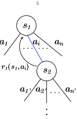
Figure 1.3: For every encountered state (si), the agent takes an action (ai) based a some policy and repeats this sequence until the termination of the episode (a finite sequence of state-action-reward triplets). After each action, (say the agent takes action ai from s1)

the agent receives a local reward. As we will discuss in greater details in chapter 3, in the case of quantum state preparation, we choose the state (s) to be the current value of the control fieldh(t) and the timet: s_{∈ {}h(t), t_}. The action is taken to be an update to the control field: h(t+ 1)←h(t) +δh,a∈ {δh}, at the following time-step. Finally, a reward is obtained only at the last step of the episode and is given by the fidelity (see Eq.1.2).

ramp time interchangeably throughout this thesis. Thus, the problem of quantum state preparation becomes that of optimizing Eq.1.2 over the space of protocols. As we will see in chapter 3, depending on the value of T, the ground-state of Eq.1.2 undergoes a variety of phase transitions and exhibits a glassy phase reminiscent of spin-glass physics and constraint satisfiability (see Fig. – to be added)

Organization of the thesis The rest of this thesis is organized as follow. In chapter2

we discuss some core principles of machine learning, along with supervised learning, unsu-pervised learning and reinforcement learning in the context of quantum state preparation. In chapter3we first discuss the problem of preparing a two-level (single qubit) system and various insights that carry on to the many-body system. We then discuss the problem of

(20)

6

preparing a periodic chain of qubits and establish a generic phase diagram for quantum control where each phases are characterized and put in correspondence with spin-glasses and constraint satisfiability problems. Finally, in chapter 4, we describe the problem of identifying in an unsupervised way clusters in raw data and describe a novel clustering algorithm which accomplishes this task.

(21)

Chapter 2

A brief overview of some important topics in

machine learning

In this chapter we discuss some important concepts pertaining to machine learning. This chapter also establishes the basic terms and notations that we will use throughout this thesis when discussing machine learning. This chapter is based on our contribution to [4], but also draws from [26] and [27].

2.1 Intuition from Statistical Learning Theory and supervised learning Supervised learning is centered around the following task: given an unknown function

y=f(x) and a fixedhypothesis set _Hconsisting of all functions we are willing to consider, we want to find the function from the hypothesis seth_{∈ H}which best approximatesf(x). Generally, we are given a set of N observations pairs: Xtrain ={(xi, yi)}Ni=0, generated by

f. Learning is referred to as the process of finding anhwhich approximatesf well over the set of observations but is also able to generalize well. The idea of generalization is central to machine learning and means that we want to find an h which approximatesf over the training set Xtrain with a performance comparable to usingh to approximatef over atest

set Xtest of previously unseen observation pairs. It is often the case the that hypothesis

set is parametrized by a set of parameters θ _∈Rp, where p is the number of parameters. For instance, in the case of a neural network, θ are the weights and biases of the neural network. In appendix A we give specific examples of supervised learning using classifiers such as logistic regression and Naive Bayes.

(22)

8

We can quantify the performance of the approximation using an objective function (which we denote E, for error) using the sum of squared errors in the case of regression problems for instance. Given an h, a training Xtrain and a test set Xtest, we can thus

compute estimates for what we will refer to as the in-sample (Ein) and out-of-sample

(Eout) error respectively. For instance, using mean-square error, we have:

Ein∼ X (xi,yi)∈Xtrain (h(xi)−yi)2, (2.1) Eout ∼ X (xi,yi)∈Xtest (h(xi)−yi)2, (2.2)

where we used _∼ to denote that these are estimates of the in-sample and out-of-sample error. In the context of supervised learning, the out-of-sample error is also referred to as the generalization error. As opposed to fitting, which is concerned only with optimizing

Ein, in supervised learning we also seek to have good performance forEout. In the following

section we will see some of the important concepts regarding how learning is different from fitting.

2.1.1 The model error versus the amount of training data

Fig. 2.1shows the typical behavior of the in-sample (Ein) and out-of-sample Eout error as

a function of the amount of training data for a fixed modelh. Typically, as the number of data point increases, the out-of-sample error decreases while the in-sample error increases, with both errors converging to the same value asymptotically. Here we have assumed that

h can never perfectly fit f(x), even in the limit of infinite data. The out-of-sample error decomposes into two terms: the bias and the variance. The bias constitutes the asymptotic error that h makes in approximating f given an infinite amount of data. The variance is related to the sampling noise of the observational training data and shrinks to zero in the limit of infinite data.

(23)

Number of data points

Error

E

in

E

out

{

<latexit sha1_base64="RG03HEwJX1WBjc+2nWlsTV1XmgQ=">AAAB6XicbVBNS8NAEJ3Ur1q/oh69LBbBU0lE0GPRi8cq9gPaUDbbSbt0swm7G6GE/gMvHhTx6j/y5r9x2+agrQ8GHu/NMDMvTAXXxvO+ndLa+sbmVnm7srO7t3/gHh61dJIphk2WiER1QqpRcIlNw43ATqqQxqHAdji+nfntJ1SaJ/LRTFIMYjqUPOKMGis99PK+W/Vq3hxklfgFqUKBRt/96g0SlsUoDRNU667vpSbIqTKcCZxWepnGlLIxHWLXUklj1EE+v3RKzqwyIFGibElD5urviZzGWk/i0HbG1Iz0sjcT//O6mYmug5zLNDMo2WJRlAliEjJ7mwy4QmbExBLKFLe3EjaiijJjw6nYEPzll1dJ66LmezX//rJavyniKMMJnMI5+HAFdbiDBjSBQQTP8Apvzth5cd6dj0VrySlmjuEPnM8fm4SNZQ==</latexit><latexit sha1_base64="RG03HEwJX1WBjc+2nWlsTV1XmgQ=">AAAB6XicbVBNS8NAEJ3Ur1q/oh69LBbBU0lE0GPRi8cq9gPaUDbbSbt0swm7G6GE/gMvHhTx6j/y5r9x2+agrQ8GHu/NMDMvTAXXxvO+ndLa+sbmVnm7srO7t3/gHh61dJIphk2WiER1QqpRcIlNw43ATqqQxqHAdji+nfntJ1SaJ/LRTFIMYjqUPOKMGis99PK+W/Vq3hxklfgFqUKBRt/96g0SlsUoDRNU667vpSbIqTKcCZxWepnGlLIxHWLXUklj1EE+v3RKzqwyIFGibElD5urviZzGWk/i0HbG1Iz0sjcT//O6mYmug5zLNDMo2WJRlAliEjJ7mwy4QmbExBLKFLe3EjaiijJjw6nYEPzll1dJ66LmezX//rJavyniKMMJnMI5+HAFdbiDBjSBQQTP8Apvzth5cd6dj0VrySlmjuEPnM8fm4SNZQ==</latexit><latexit sha1_base64="RG03HEwJX1WBjc+2nWlsTV1XmgQ=">AAAB6XicbVBNS8NAEJ3Ur1q/oh69LBbBU0lE0GPRi8cq9gPaUDbbSbt0swm7G6GE/gMvHhTx6j/y5r9x2+agrQ8GHu/NMDMvTAXXxvO+ndLa+sbmVnm7srO7t3/gHh61dJIphk2WiER1QqpRcIlNw43ATqqQxqHAdji+nfntJ1SaJ/LRTFIMYjqUPOKMGis99PK+W/Vq3hxklfgFqUKBRt/96g0SlsUoDRNU667vpSbIqTKcCZxWepnGlLIxHWLXUklj1EE+v3RKzqwyIFGibElD5urviZzGWk/i0HbG1Iz0sjcT//O6mYmug5zLNDMo2WJRlAliEjJ7mwy4QmbExBLKFLe3EjaiijJjw6nYEPzll1dJ66LmezX//rJavyniKMMJnMI5+HAFdbiDBjSBQQTP8Apvzth5cd6dj0VrySlmjuEPnM8fm4SNZQ==</latexit><latexit sha1_base64="RG03HEwJX1WBjc+2nWlsTV1XmgQ=">AAAB6XicbVBNS8NAEJ3Ur1q/oh69LBbBU0lE0GPRi8cq9gPaUDbbSbt0swm7G6GE/gMvHhTx6j/y5r9x2+agrQ8GHu/NMDMvTAXXxvO+ndLa+sbmVnm7srO7t3/gHh61dJIphk2WiER1QqpRcIlNw43ATqqQxqHAdji+nfntJ1SaJ/LRTFIMYjqUPOKMGis99PK+W/Vq3hxklfgFqUKBRt/96g0SlsUoDRNU667vpSbIqTKcCZxWepnGlLIxHWLXUklj1EE+v3RKzqwyIFGibElD5urviZzGWk/i0HbG1Iz0sjcT//O6mYmug5zLNDMo2WJRlAliEjJ7mwy4QmbExBLKFLe3EjaiijJjw6nYEPzll1dJ66LmezX//rJavyniKMMJnMI5+HAFdbiDBjSBQQTP8Apvzth5cd6dj0VrySlmjuEPnM8fm4SNZQ==</latexit>

Bias

{

<latexit sha1_base64="RG03HEwJX1WBjc+2nWlsTV1XmgQ=">AAAB6XicbVBNS8NAEJ3Ur1q/oh69LBbBU0lE0GPRi8cq9gPaUDbbSbt0swm7G6GE/gMvHhTx6j/y5r9x2+agrQ8GHu/NMDMvTAXXxvO+ndLa+sbmVnm7srO7t3/gHh61dJIphk2WiER1QqpRcIlNw43ATqqQxqHAdji+nfntJ1SaJ/LRTFIMYjqUPOKMGis99PK+W/Vq3hxklfgFqUKBRt/96g0SlsUoDRNU667vpSbIqTKcCZxWepnGlLIxHWLXUklj1EE+v3RKzqwyIFGibElD5urviZzGWk/i0HbG1Iz0sjcT//O6mYmug5zLNDMo2WJRlAliEjJ7mwy4QmbExBLKFLe3EjaiijJjw6nYEPzll1dJ66LmezX//rJavyniKMMJnMI5+HAFdbiDBjSBQQTP8Apvzth5cd6dj0VrySlmjuEPnM8fm4SNZQ==</latexit><latexit sha1_base64="RG03HEwJX1WBjc+2nWlsTV1XmgQ=">AAAB6XicbVBNS8NAEJ3Ur1q/oh69LBbBU0lE0GPRi8cq9gPaUDbbSbt0swm7G6GE/gMvHhTx6j/y5r9x2+agrQ8GHu/NMDMvTAXXxvO+ndLa+sbmVnm7srO7t3/gHh61dJIphk2WiER1QqpRcIlNw43ATqqQxqHAdji+nfntJ1SaJ/LRTFIMYjqUPOKMGis99PK+W/Vq3hxklfgFqUKBRt/96g0SlsUoDRNU667vpSbIqTKcCZxWepnGlLIxHWLXUklj1EE+v3RKzqwyIFGibElD5urviZzGWk/i0HbG1Iz0sjcT//O6mYmug5zLNDMo2WJRlAliEjJ7mwy4QmbExBLKFLe3EjaiijJjw6nYEPzll1dJ66LmezX//rJavyniKMMJnMI5+HAFdbiDBjSBQQTP8Apvzth5cd6dj0VrySlmjuEPnM8fm4SNZQ==</latexit><latexit sha1_base64="RG03HEwJX1WBjc+2nWlsTV1XmgQ=">AAAB6XicbVBNS8NAEJ3Ur1q/oh69LBbBU0lE0GPRi8cq9gPaUDbbSbt0swm7G6GE/gMvHhTx6j/y5r9x2+agrQ8GHu/NMDMvTAXXxvO+ndLa+sbmVnm7srO7t3/gHh61dJIphk2WiER1QqpRcIlNw43ATqqQxqHAdji+nfntJ1SaJ/LRTFIMYjqUPOKMGis99PK+W/Vq3hxklfgFqUKBRt/96g0SlsUoDRNU667vpSbIqTKcCZxWepnGlLIxHWLXUklj1EE+v3RKzqwyIFGibElD5urviZzGWk/i0HbG1Iz0sjcT//O6mYmug5zLNDMo2WJRlAliEjJ7mwy4QmbExBLKFLe3EjaiijJjw6nYEPzll1dJ66LmezX//rJavyniKMMJnMI5+HAFdbiDBjSBQQTP8Apvzth5cd6dj0VrySlmjuEPnM8fm4SNZQ==</latexit><latexit sha1_base64="RG03HEwJX1WBjc+2nWlsTV1XmgQ=">AAAB6XicbVBNS8NAEJ3Ur1q/oh69LBbBU0lE0GPRi8cq9gPaUDbbSbt0swm7G6GE/gMvHhTx6j/y5r9x2+agrQ8GHu/NMDMvTAXXxvO+ndLa+sbmVnm7srO7t3/gHh61dJIphk2WiER1QqpRcIlNw43ATqqQxqHAdji+nfntJ1SaJ/LRTFIMYjqUPOKMGis99PK+W/Vq3hxklfgFqUKBRt/96g0SlsUoDRNU667vpSbIqTKcCZxWepnGlLIxHWLXUklj1EE+v3RKzqwyIFGibElD5urviZzGWk/i0HbG1Iz0sjcT//O6mYmug5zLNDMo2WJRlAliEjJ7mwy4QmbExBLKFLe3EjaiijJjw6nYEPzll1dJ66LmezX//rJavyniKMMJnMI5+HAFdbiDBjSBQQTP8Apvzth5cd6dj0VrySlmjuEPnM8fm4SNZQ==</latexit>

Variance

Figure 2.1: Schematic of the typical in-sample and out-of-sample error as a function of training set size. The typical in-sample or training error, Ein, the

out-of-sample or generalization error,Eout, the bias and the variance as a function of the number

of training data points. The schematic assumes that the number of data points is large.

of training data. The bias is thus a property of the model itself and in general more complex models, that is (as a rule of thumb), model with more parameters, will have a smaller biases1_{. Another quantity of interest in Fig.} _2.1 _{is the difference} _|_E

out −Ein|

which can be thought as a measure of how well the in-sample fitting captures the out-of-sample predictions. Models with a large discrepancy between the training error and the generalization error are said to overfit the data. In other words, these models tend to put too much emphasis on the training data and do not generalize well. An extreme limit of this is learning by heart, that is, repeating previously observed target datayi if given the

1_{Note that models with more parameters are not always more complex. For a more thorough discussion}

(24)

10

Model complexity

Error

E

out

Bias

Variance

Optimal complexity

Figure 2.2: Bias-Variance tradeoff and model complexity. This schematic shows the typical out-of-sample error Eout as function of the model complexity for a training dataset of fixed size. Notice how the bias always decreases with model complexity, but the variance, i.e. fluctuation in performance due to finite size sampling effects, increases with model complexity. Thus, optimal performance is achieved at intermediate levels of model complexity.

samexi and a random yi otherwise. Learning to generalize well by only using the training data is the central goal of machine learning.

2.1.2 The model error versus the model’s complexity

The second schematic, shown in Figure 2.2, shows the out-of-sample, or test, error Eout

as function of “model complexity”. Model complexity is a very subtle idea and defining it precisely is one of the great achievements of statistical learning theory. However, roughly speaking, model complexity is a measure of the complexity of the model class we are using to approximate the true function f(x). For example, a model with more free parameters

(25)

is generally more complex than one with fewer fitting parameters2_{. In the example of}

polynomial regression discussed above, higher-order polynomials are more complex than the linear model. If we consider a training dataset of a fixed size, Eout will be a

non-monotonic function of the model complexity, and is generally minimized for models with intermediate complexity. The underlying reason for this is that, even though using a more complicated model always reduces the bias, at some point the model becomes too complex for the amount of training data and the generalization error becomes large due to high variance. Thus, to minimize Eout and maximize our predictive power, it may be more

suitable to use a more biased model with small variance than a less-biased model with large variance. This important concept is commonly called the bias-variance tradeoff and gets at the heart of why machine learning is difficult.

2.2 Unsupervised learning

2.2.1 Dimensional reduction and data visualization

In this section, we will begin our foray into unsupervised learning by way of data visual-ization. In machine learning, data visualization is an important tool to identify structures such as correlations, invariances (symmetries) or irrelevant features (noise) in raw or pro-cessed data. Conceivably, being able to capture these properties could help us design better predictive models. In practice, however, the data we are dealing with is often high-dimensional, which means that its visualization is impossible or daunting at best. Part of the complication is due to that low-dimensional representation of high-dimensional data necessarily incurs information lost.

A simple way to visualize data is through pair-wise correlations (i.e. pairwise scatter plots of all features). This is useful in highlighting important correlations between features when the number of features we are measuring is relatively small. In practice, we often have to performdimensional reduction, namely, construct a projection or an embedding of

2_{Note that models with more parameters are not always more complex. One neat example in the context}

(26)

12

the data, from the original high-dimensional space to a lower dimensional space, which we refer to as the latent space. In this section, we discuss both linear and nonlinear methods for dimensional reduction with applications in data visualization. We note that beyond data visualization, the techniques introduced in this section can be used in many other applications such as lossy data compression and feature extraction.

2.2.2 Some of the challenges of high-dimensional data

Before we discuss specific dimensional reduction techniques, we first highlight some of the difficulties in dealing with high-dimensional data.

High-dimensional data lives near the edge of sample space Geometry in high-dimensional space can be counterintuitive. One example that is pertinent to machine learn-ing is the followlearn-ing. Consider data distributed uniformly at random in a D-dimensional hypercube C = [−e/2, e/2]D, where e is the edge length. Consider also a D-dimensional hypersphereSof radiuse/2 centered at the origin and contained withinC. The probability that a data pointxdrawn uniformly at random in _C is contained within_S is well approx-imated by the ratio of the volume of _S to that of _C : p(_kx_k₂ < e/2) _∼ (1/2)D_{. Thus,} as the dimension of the feature space D increases, p goes to zero exponentially fast. In other words, most of the data will concentrate outside the hypersphere, in the corners of the hypercube. In physics, this basic observation underlies many properties of ideal gases such as the Maxwell distribution and the equipartition theorem (see Chapter 3 of [28] for instance).

Real-world data vs. uniform distribution Fortunately, real-world data is not random or uniformly distributed! In fact, real data usually lives in a much lower dimensional space than the original space in which the features are being measured (see Fig. 2.3). This is sometimes referred to as the “blessing of non-uniformity” (in opposition to the curse of dimensionality). Data will typically be locally smooth, meaning that a local variation of the

(27)

data will not incur a change in the target variable [27]. This idea is similar to statistical physics where properties of most systems with many degrees of freedom can often be characterized by low-dimensional “order parameters”. In thermodynamics, bulk properties of a gas of weakly interacting particles can be simply described by the thermodynamic variables that enter equation of states rather than the astronomically large dynamical variables (i.e. position and momentum) of each particle in the gas is another instantiation of this idea.

a)

b)

Figure 2.3: Data distributed in a three dimensional space (a) that can effectively be de-scribed on a two-dimensional surface (b). A common goal of dimensional reduction is to preserve the local structure in the data. The embedding of (a) to (b) preserves the local structure of the data as can be seen by inspecting the color gradient.

The crowding problem When performing dimensional reduction, a common goal is to preserve pairwise distances between data points from the original space to the latent space. This can be achieved fairly well if the intrinsic dimensionality of the data is the same as the dimension of the latent space [29]. Consider for instance the example of the Swiss roll (see Fig. 2.3). The intrinsic dimensionality of the Swiss roll is approximately 2 and as such it can be well represented in a two dimensional space.

If one attempts to represent data in a space with dimensionality lower than it’s intrinsic dimensionality while preserving too much information, a problem known as the “crowding

(28)

14

problem” can occur [29] (see schematic, Fig. 2.4). Intuitively this is a consequence of the following: in a D dimensional space on can construct objects of N = D+ 1 multually equidistant points (equilateral triangle inD= 2, the tetrahedron inD= 3, etc.). If we try to construct an equivalent object in D0 < D by requiring that all distances between the points are equal, the points would collapse onto one another.

To alleviate this, one needs to weaken the constraint we impose on our visualization schemes. For instance, in the case of t-distributed stochastic neighbor embedding (t-SNE) [29], see below, rather than trying to preserve all relative pairwise distances, one prioritizes the preservation of local structure in the data.

2D

1D

Figure 2.4: Illustration of the crowding problem. (left) Consider an origina[h!]l space in 2 dimensions with three pairwise equidistant points. (right) Mapped space: if one wants to preserves the ordination or distances in a 1D space exactly, all points must collapse onto one another.

2.2.3 Principal component analysis (PCA)

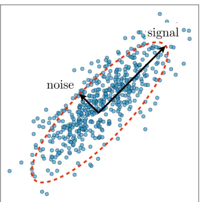
One of the most commonly used dimensional reduction and visualization techniques is Principal Component Analysis (PCA). The goal of PCA is to perform a linear projection of the data onto a lower-dimensional subspace where the variance is maximized. PCA is inspired by the observation that in many cases relevant information is often contained in the directions with largest variance (see Fig. 2.5). Intuitively, these directions encode the

(29)

noise

signal

Figure 2.5: PCA seeks to find the set of orthogonal directions for which that data has the largest variance. For the case of 2D data, this can be seen as “fitting” an ellipse to the data with the major axis corresponding to the first principal component (direction of largest variance). Directions with large variance are usually interpreted as the signal in the data while directions with low variance are attributed to noise.

large-scale “signal” as opposed to “noise” characterized by the direction of small variance. PCA also seeks variable directions while simultaneously reducing the redundancy between the new basis vectors [30]. This is done by requiring our new basis vectors (called principal components) to be orthogonal. The data is then visualized by projecting it onto a subspace spanned by a few principal component basis vectors.

Surprisingly, such PCA-based projections often capture a lot of the large scale struc-ture of many datasets. For example, Figure 2.6 shows the projection of samples drawn from the 2D Ising model at various temperatures on the first two principal components. Despite living in a 1600 dimensional space (the samples are 40×40 spins), a single principal component (i.e. a single direction in this 1600 dimensional space) can capture 50% of the variability contained in our samples. In fact, one can verify that this direction weights

(30)

16

Figure 2.6: (a) The first 2 principal component of the Ising dataset (see appendixBfor more detail on the dataset) with temperature indicated by the coloring. PCA was performed on a joined dataset of 1000 samples taken at each temperaturesT = 0.25,0.5,· · ·,4.0. Almost all the variance is explained in the first component which corresponds to the magnetiza-tion order parameter (linear combinamagnetiza-tion of the features with weights all roughly equal). The paramagnetic phase corresponds to the middle cluster and the left and right clusters correspond to the symmetry-related ferromagnetic phases (b) Log of the spectrum of the covariance matrix versus rank ordering. Only one dimension has high-variance.

(31)

all 1600 spins nearly equally and thus corresponds to the magnetization order parameter. Thus, even without any prior physical knowledge, one can extract relevant order parame-ters using a simple PCA-based projection. PCA is widely employed in biological physics when working with high-dimensional data. Recently, a correspondence between PCA and Renormalization Group flows across the phase transition in the 2D Ising model [31] or in a general setting [32] has been proposed. In statistical physics, PCA has also found applica-tion in detecting phase transiapplica-tions [33], e.g. in the XY model on frustrated triangular and union jack lattices [34]. It was also used to classify dislocation patterns in crystals [35,36]. Physics has also inspired PCA-based algorithms to infer relevant features in unlabelled data [37].

Concretely, consider N data points, {x1, . . .xN} that live in a D-dimensional feature space RD. Without loss of generality, we assume that the empirical mean ¯x=N−1P_ixi of these data points is zero3_{. Denote the} _N _×_D _{design matrix as} _X _{= [}_x

1,x2, . . .;xN]T whose rows are the data points and columns correspond to different features. TheD_×D

(symmetric) covariance matrix is therefore

Σ(X) = 1

N −1X

T_X_. _(2.3)

Notice that thej-th diagonal entry ofΣ(X) corresponds to the variance of thej-th feature andΣ(X)ij measures the covariance (i.e. connected correlation in the language of physics) between featureiand feature j.

We are interested in finding a new basis for the data that emphasizes highly variable directions while reducing redundancy between basis vectors. In particular, we will look for a linear transformation that reduces the covariance between different features. To do so, we first perform singular value decomposition (SVD) on the design matrixX, namely,

X =U SVT, where S is a diagonal matrix of singular value si, the orthogonal matrix U contains (as its columns) the left singular vectors of X, and similarly V contains (as its

3_{We can always center around the mean: ¯}_x

(32)

18

columns) the right singular vectors ofX. With this, one can rewrite the covariance matrix as Σ(X) = 1 N₋1V SU T_{U SV}T = V S2 N −1 VT ≡ VΛVT. (2.4)

whereΛis a diagonal matrix with eigenvaluesλi in the decreasing order along the diagonal (i.e. eigendecomposition). It is clear that the right singular vectors ofX (i.e. columns ofV) are principal directions ofΣ(X), and the singular values ofX are related to the eigenvalues of the covariance matrixΣ(X) viaλi=s2_i/(N−1). To reduce the dimensionality of data

from D to ˜D < D, we first construct the D×D˜ projection matrix ˜V_D0 by selecting the

singular components with the ˜D largest singular values. The projection of the data from

Dto a ˜D dimensional space is simply ˜Y =XV˜D0.

The singular vector with the largest singular value (i.e the largest variance) is referred to as the first principal component, the singular vector with the second largest singular value as the second principal component, and so on. An important quantity is the ratio

λi/PDi=1λi which is referred as the percentage of the explained variance contained in a

principal component (see Fig. 2.6.b).

It is common in data visualization to present the data projected on the first few principal components. This is valid as long as a large part of the variance is explained in those components. Low values of explained variance may imply that the intrinsic dimensionality of the data is high or simply that it cannot be captured by a linear representation. For a detailed introduction to PCA, see the introductory tutorial by Shlens [30] or Bishop [27].

(33)

2.2.4 Multidimensional scaling

Multidimensional scaling (MDS) is a non-linear dimensional reduction technique which preserves the pairwise distance or dissimilarity dij between data points [38]. Moving for-ward, we use the term “distance” and “dissimilarity” interchangeably. There are two types of MDS: metric and non-metric. In metric MDS, the distance matrix is computed under a pre-defined metric and the latent coordinatesY˜ are obtained by minimizing the difference between the distance matrix in the original space (dij(X)) and that in the latent space (dij(Y)): ˜ Y = arg min Y X i<j wij|dij(X)−dij(Y)|, (2.5)

where wij is a weight value: wij ≥ 0. The weight matrix wij is a set of free parameters that specify the level of confidence (or precision) in the value of dij(X). If Euclidean metric is used, it is the same as PCA and is usually referred to as classical scaling [39]. Thus MDS is often considered as a generalization of PCA. In non-metric MDS, dij can be any distance matrix. The objective function is then to preserve the ordination in the data, i.e. if d12(X) < d13(X) in the original space, then in the latent space we should

have d12(Y) < d13(Y). Both MDS and PCA can be implemented using standard Python

packages such as Scikit. MDS algorithms typically have a scaling of O(N3_{) where} _N

corresponds to the number of data points, and thus is very limited in it’s application to large datasets. However, sample-based methods have been introduce to reduce this scaling to a much reasonable _O(NlogN) scaling [40]. In the case of PCA, a complete decomposition has a scaling of _O(N p2₊_p3_{) and can be improved to} _O₍_{N p}2₊_p_{) if only}

the first few principal components are desired (using iterative approaches). PCA and MDS are often among the first data visualization techniques one resorts to.

2.2.5 t-SNE

It is often desirable to preserve local structures in high-dimensional datasets. However, when dealing with datasets having clusters delimitated by complicated decision surfaces

(34)

20

or datasets with a large number of clusters, preserving local structures become difficult using linear techniques such as PCA. Many non-linear techniques such as non-classical MDS [38], self-organizing map [41], Isomap [42] and Locally Linear Embedding [43] have been proposed and to address this class of problems. These techniques are generally good at preserving local structures in the data but typically fail to capture structures at the larger scale such as the clusters in which the data is organized[29]. Recently, t-stochastic neighbor embedding (t-SNE) has emerged as one of the go-to methods for visualizing high-dimensional data. It has been shown to offer insightful visualization for many benchmark high-dimensional datasets [29].

t-SNE is a non-parametric4 _{method that constructs non-linear embeddings. Each}

high-dimensional training point is mapped to low-high-dimensional embedding coordinates, which are optimized in a way to preserve the local structure in the data.

When used appropriately,t-SNE is a powerful technique for unraveling the hidden struc-ture of high-dimensional datasets while at the same time preserving locality. In physics,

t-SNE has recently been used to reduce the dimensionality and classify spin configurations, generated with the help of Monte Carlo simulations, for the Ising [44] and Fermi-Hubbard models at finite temperatures [45]. It was also applied to study clustering transitions in glass-like problems in the context of quantum control [46].

The idea of stochastic neighbor embedding is to associate a probability distribution to the neighborhood of each data point (notex∈Rs,sis the number of features):

p_i|j =

exp(−||xi−xj||2/2σi2)

P

k6=iexp(−||xi−xk||2/2σi2)

, (2.6)

wherep_i|jcan be interpreted as the likelihood thatxjisxi’s neighbor (thus we takepi|i= 0).

σi are free bandwidth parameters that are usually determined by fixing the local entropy

4_{It does not explicitly parametrize feature extraction required to compute the embedding coordinates.}

(35)

H(pi) of each data point:

H(pi)≡ −

X

j

pj|ilog2pj|i. (2.7)

The local entropy is then set to be a constant acrossall data points Σ = 2H(pi)_{, where Σ is}

called the perplexity. The perplexity constraint determines σi ∀ iand implies that points in regions of high-density will have smallerσi.

The using of Gaussian likelihoods in p_i|j implies that only points that are nearby xi contribute to its probability distribution. While this ensures that the similarity for nearby points is well represented, this can be a problem for outliers which will have exponentially vanishing contributions forallpoints, which in turn mean that their embedding coordinates are ambiguous [29]. A way around this is to define symmetrized distribution pij ≡(pi|j+

p_j|i)/(2N) which satisfies Pjpij >1/(2N) for all data pointsxi.

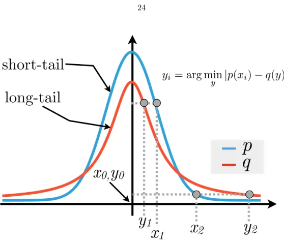
t-SNE constructs an equivalent probability distribution qij in a low dimensional latent space (with coordinates Y = _{yi}, yi ∈ Rt, where t < s is the dimension of the latent space): qij = (1 +||yi−yj||2)−1 P k6=i(1 +||yi−yk||2)−1 . (2.8)

The crucial point to note is that qij is chosen to be a long tail distribution. This preserve short distance information (relative neighborhoods) while strongly repelling two points that are far apart in the original space (see Fig. 2.7). In order to find the latent space coordinatesyi, t-SNE minimizes the Kullback-Leibler divergence between qij and pij:

C(Y) =KL(p_||q)_≡X ij pijlog pij qij . (2.9)

This minimization is done via gradient descent. We can gain further insights on what the embedding cost-functionCis capturing by computing the gradient of (2.9) with respect to

(36)

22 yi explicitly: ∂iC= X j6=i 4pijqijZi(yi−yj)− X j6=i 4q_ij2Zi(yi−yj), (2.10) =Fattractive,i−Frepulsive,i, (2.11)

where Zi = 1/(Pk6=i(1 +||yk−yi||2)−1). We have divided the gradient of point yi into an attractive Fattractive and repulsive term Frepulsive. Remark that Fattractive,i induces a significant attractive force only between points that are nearby pointiin theoriginal space since it involves the pij term. Finding the embedding coordinates yi is thus equivalent to finding the equilibrium configuration of particles interacting through the forces in (2.11).

Here we list some important properties that one should bear in mind when analyzing

t-SNE plots.

• t-SNE can rotate data. The KL divergence is invariant under rotations in the latent space, since it only depend