DCASE 2019 TASK 2: MULTITASK LEARNING, SEMI-SUPERVISED LEARNING AND
MODEL ENSEMBLE WITH NOISY DATA FOR AUDIO TAGGING
Osamu Akiyama
and Junya Sato
Faculty of Medicine, Osaka University, Osaka, Japan
{oakiyama1986, junya.sto}@gmail.com
ABSTRACT
This paper describes our approach to the DCASE 2019 challenge Task 2: Audio tagging with noisy labels and minimal supervision. This task is a multi-label audio classification with 80 classes. The training data is composed of a small amount of reliably labeled data (curated data) and a larger amount of data with unreliable labels (noisy data). Additionally, there is a difference in data dis-tribution between curated data and noisy data. To tackle these dif-ficulties, we propose three strategies. The first is multitask learn-ing uslearn-ing noisy data. The second is semi-supervised learnlearn-ing us-ing noisy data and labels that are relabeled usus-ing trained models’ predictions. The third is an ensemble method that averages mod-els trained with different time length. By using these methods, our solution was ranked in 3rd place on the public leaderboard (LB) with a label-weighted label-ranking average precision (lwlrap) score of 0.750 and ranked in 4th place on the private LB with a lwlrap score of 0.75787. The code of our solution is available at https://github.com/OsciiArt/Freesound-Audio-Tagging-2019.
Index Terms— Audio-Tagging, Noisy Labels, Multitask Learn-ing, Semi-supervised LearnLearn-ing, Model Ensemble
1. INTRODUCTION
An automatic general-purpose audio tagging system can be useful for various usages, including sound annotating or video caption-ing. However, there are no such systems with adequate perfor-mance because of the difficulty of this task. To build such a sys-tem using machine learning techniques, an audio dataset with re-liable labels is required. However, it is difficult to obtain large-scale dataset with reliable labels because manual annotation by humans is time-consuming. In contrast, it is easy to infer labels automatically using metadata of websites like Freesound [1] or Flickr [2] that collect audio and metadata from collaborators. Nevertheless, automatically inferred labels are inevitable to have a certain amount of label noise.
DCASE 2019 challenge Task 2: Audio tagging with noisy la-bels and minimal supervision [3] is a multi-label audio classifica-tion task with 80 classes. The FSDKaggle2019 dataset was pro-vided for this challenge. The main motivation of this task is to fa-cilitate research of audio classification leveraging a small amount of reliably labeled data (curated data) and a larger amount of data with unreliable labels (noisy data) with a large number of catego-ries.
This work was supported by Osaka University Medical Doctor Scientist Training Program.
This task has three main challenges. First, this is a multi-label classification task, which is more difficult than a single-label clas-sification task. Second, most of the training data labels are so un-reliable that the performance of a classification model trained with them would be lower than a one trained without them. Third, there is a difference in data distribution between curated data and noisy data because they come from different sources. Therefore, domain adaptation approaches would be required.
2. OUR PROPOSALS
2.1. MULTITASK LEARNING
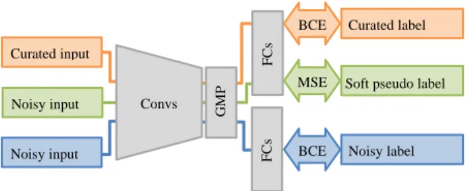
In this task, the curated data and noisy data are labeled in a differ-ent manner, therefore treating them as the same one makes the model performance worse. To tackle this problem, we used a mul-titask learning approach [4, 5], in which a model learns multiple tasks simultaneously. The aim of multitask learning is to get a more generalized model by learning representations shared be-tween 2 tasks. We treated learning with curated data and noisy data as different tasks and performed multitask learning. In our proposal, a convolution layer architecture learns the feature rep-resentations shared between curated and noisy data, and the two separated sequences of full-connect (FC) layers learn the differ-ence between the two data (Fig. 1). In this way, we can get the advantages of representation learning from noisy data and avoid the disadvantages of noisy label perturbation. We set the loss weight ratio of curated and noisy as 1:1.
2.2. SEMI-SUPERVISED LEARNING
Because treating the noisy labels the same as the curated labels makes the model performance worse, it may be promising to do semi-supervised learning [6] (SSL) using the noisy data without the noisy labels. However, this task is different from the data that SSL is generally applied in two points. The first, there is a differ-ence in data distribution between labeled data and unlabeled data. It is reported that applying SSL to such data makes model perfor-mance worse [6]. The second, this is a multi-label classification task. Most of SSL methods are for single-label classification task. We tried Pseudo-Label [7], Mean Teacher [8], and MixMatch [9] and all of them were not successful in improving lwlrap score. In the original Pseudo-Label, guessed labels are made from predic-tions of the training model itself, but we made guessed labels from trained models because it is a popular approach.
Therefore, we propose an SSL method that is robust to data distribution difference and can handle multi-label data (Fig. 1). For each noisy data sample, we guess the label using trained models. The guessed label is processed by a sharpening function [9], which sharpens the predicted categorical distribution by adjusting the
“temperature.” We call this soft pseudo label. The basic Pseudo-Label is a hard label with only one positive label so that it cannot apply to multi-label data. In contrast, the soft pseudo label is sharp-ened label distribution and suits for multi-label data. The soft pseudo label is expected to be more robust to data distribution dif-ference because it is smoother than the hard label. Learning with soft pseudo labels is performed in parallel with multitask learning. As the temperature of the sharpening function, we tried a value of 1, 1.5, and 2. A value of 2 was the optimum. The predictions used for the guessed labels were obtained from a ResNet model with multitask learning (Table 1 #4) using Snapshot Ensembles [10] and 5-fold cross validation (CV) averaging with all the folds and cycle snapshots of 5-fold CV. We used mean squared error (MSE) as a loss function. We set loss weight of SSL as 20. To get the benefit of mixup [11] more, we mixed curated data and its label to soft pseudo label data with a ratio of 1:1.
2.3. ENSEMBLE
To obtain the benefit of ensemble, we prepared models trained with various conditions and averaged the categorical dis-tribution predicted by the models with weighted ratio (model av-eraging). As the variety of models, we employed 5-fold CV aver-aging, Snapshot Ensembles [10] and models trained with wave-form or log mel spectrogram. K-fold CV averaging is averaging of predictions of all the models of k-fold CV on the test data. Snapshot Ensembles is averaging of predictions of model snap-shots which is model weights of each cycle's end in model training with cyclic cosine learning rate [12]. As an approach specific to this competition data, we averaged models trained with different cropping length of time, we call this cropping length averaging. There is a difference in time length average among classes. There-fore, models trained with different time length are expected to be-come experts for different classes, and they give a variety to the model ensemble.
3. METHODOLOGY
3.1. DATASET
The FSDKaggle2019 dataset was provided for this challenge [3]. This dataset consists of four subsets: curated train data with 4,970 audio samples, noisy train data with 19,815 samples, public test data with 1,120 samples, and private test data with 3,361 samples. Each audio sample is labeled with 80 classes, including human sounds, domestic sounds, musical instruments, vehicles, and ani-mals. Curated train data and test data are collected from Freesound dataset [1] and labeled manually by humans. Noisy train data is collected from Yahoo Flickr Creative Commons 100M dataset (YFCC) [2] and labeled using automated heuristics applied to the audio content and metadata of the original Flickr clips. All audio samples are single-channel waveforms with a sampling rate of 44.1kHz. In curated data, the duration of the audio samples ranges from 0.3 to 30 second, and the number of clips per class is 75,
Figure 1: Overall architecture of our proposed model. The model is trained with three methods concurrently. (1) Basic classification (2) Soft pseudo label (3) Multitask learning with noisy label. Conv: convolution layer, GMP: global max pooling, FC: full-con-nect layers, BCE: binary cross-entropy, MSE: mean squared error.
except in a few cases. In noisy data, the duration of the audio sam-ples ranges from 1 to 15 second, and the number of clips per class is 300, except in a few cases.
3.2. PREPROCESSING
We used both waveform and log mel spectrogram as input data. These two data types are expected to compensate for each other.
3.2.1.Waveform
We tried a sampling rate of 44.1 kHz (original data) and 22.05 kHz, and we found that 44.1 kHz was better. Each input data was regu-larized into a range of from -1 to +1 by dividing by 32,768, the full range of 16-bit audio.
3.2.2.Log mel spectrogram
For the log mel spectrogram transformation, we used 128 mel fre-quency channels. We tried 64 and 256, but model performance decreased. We used the short-time Fourier transform hop size of 347 that makes log mel spectrogram 128 Hz time resolution. Data samples of the log mel spectrogram were converted from power to dB after all augmentations were applied. After that, each data sample was normalized with the mean and standard deviation of each single data sample. Therefore, the mean and standard devia-tion values change every time, and this works as a kind of aug-mentation. Normalization using the mean and standard deviation of all the data decreased model performance.
3.3. AUGMENTATIONS
3.3.1.Augmentations for log mel spectrogram
Mixup/BC learning [11, 13] is an augmentation that mixes two pairs of inputs and labels with some ratio. The mixing rate is se-lected from a Beta distribution. We set a parameter α of the Beta distribution to 1.0, which makes the Beta distribution equal to a uniform distribution. We applied mixup with a ratio of 0.5.
SpecAugment [14] is an augmentation method for log mel spectrogram consists of three kinds of deformation. The first is time warping that deforms time-series in the time direction. The other two augmentations are time and frequency masking,
Noisy label BCE
Curated label BCE
Soft pseudo label MSE Curated input (1) Noisy input (2) Noisy input (3) Convs FC s F C s G M P
modifications of Cutout [15], that masks a block of consecutive time steps or mel frequency channels. We applied frequency mask-ing, and masking width is chosen from 8 to 32 from a uniform distribution. Time warping and time masking are not effective in this task, and we did not apply them to our models. We applied frequency masking with a ratio of 0.5.
For training, audio samples which have various time lengths are converted to a fixed length by random cropping. The sound samples which have short length than the cropping length are ex-tended to the cropping length by zero paddings. We tried 2, 4, and 8 seconds (256, 512, and 1024 dimensions) as a cropping length and 4 seconds scores the best. Averaging models trained with 4-second cropping and 8-4-second cropping achieved a better score.
Expecting more strong augmentation effect, after basic crop-ping, we shorten data samples in a range of 25 - 100% of the basic cropping length by additional cropping and extend to the basic cropping length by zero padding. For data samples with a time length shorter than the basic cropping length, we shorten data samples in a range of 25 - 100% of original length by additional cropping and extend to the basic cropping length by zero paddings. We applied this additional cropping with a ratio of 0.5.
As another augmentation, we used gain augmentation with a factor randomly selected from a range of 0.80 - 1.20 with a ratio of 0.5. We tried scaling augmentation and white noise augmenta-tion, but model performance decreased.
3.3.2.Augmentations for waveform
We applied mixup to waveform input. We used a parameter α of 1.0 for the Beta distribution as same as the case of log mel spec-trogram.
We applied cropping to waveform input. We tried 1.51, 3.02, and 4.54 seconds (66,650, 133,300, and 200,000 dimen-sions) as a cropping length, and we found that 4.54 seconds is optimal. Averaging models trained with 3.02-second cropping and 4.54-second cropping achieved a better score.
We used scale augmentation with a factor randomly selected from a range of 0.8 - 1.25 and gain augmentation with a factor randomly selected from a range of 0.501 - 2.00.
3.4. MODEL ARCHITECTURE
3.4.1.ResNet
We selected ResNet [16] as a log mel spectrogram-based model because it is a widely-used image classification model and rela-tively simple. We compared ResNet18, ResNet34 and SE-ResNeXt50 [17] and ResNet34 performed the best. The number of trainable parameters, including the multitask module is 44,210,576. We applied a global max pooling (GMP) after con-volutional layers to make a model adaptive to various input length.
3.4.2.EnvNet
We selected EnvNet-v2 [13] as a waveform-based model because it is state of the art of a waveform-based model. The number of trainable parameters, including the multitask module is 4,128,912. As same as ResNet, we applied a GMP after convolutional layers to allow variable input length.
3.4.3.Multitask module
For multitask learning, two separate FC layer sequences follow after convolution layers and GMP. The contents of both se-quences are the same and consist of FC (1024 units) - ReLU - dropout [18] (drop rate = 0.2) - FC (1024 units) - ReLU - dropout (drop rate = 0.1) - FC (80 units) - sigmoid. Sigmoid is replaced by softmax in model E and F of EnvNet (Table 2).
3.5. TRAINING
3.5.1.ResNet
We used Adam [19] for optimization. We used cyclic cosine learning rate for learning rate schedule. In each cycle, the learning rate is started with 1e-3 and decrease to 1e-6. There are 64 epochs per cycle. We used a batch size of 32 or 64. We used binary cross-entropy (BCE) as a loss function for basic classification and mul-titask learning with noisy data. We used mean squared error as a loss function for the soft pseudo label. The model weights of each cycle’s end were saved and used for Snapshot Ensembles.
3.5.2.EnvNet
We used stochastic gradient descent (SGD) for optimization. We used cyclic cosine learning rate for learning rate schedule. In each cycle, the learning rate is started with 1e-1 and decrease to 1e-6. There are 80 epochs per cycle. We used binary cross-entropy as a loss function for the model using sigmoid and Kullback-Leibler divergence for the model using softmax. We used a batch size of 64 for the model using sigmoid and 16 for the model using soft-max.
3.6. POSTPROCESSING AND ENSEMBLE
Prediction using the full length of audio input scores better than prediction using test time augmentation (TTA) with cropped au-dio input. This may be because essential components for classifi-cation is concentrated on the beginning part of audio samples. Pre-diction with cropping of the beginning part scores better than pre-diction with cropping of the latter part. In order to speed up the calculation, audio samples with similar lengths were grouped, and the lengths of samples in the same group were adjusted to the same length by zero paddings and converted to mini-batches. The patience for the difference of length within a group (patience rate) was adjusted based on the prediction speed.
We found that padding augmentation is effective TTA. Padding augmentation is an augmentation method that applies zero pad-dings to both sides of audio samples with various length and av-erages prediction results. In the training phase, we applied pad-ding to input data to make the sample size the same. Because there is a correlation between time length and class, models are thought to learn that there is a correlation between padding length and class. We think that padding augmentation reduces this bias and gives better predictions.
For model averaging, we prepared models trained with var-ious conditions, as mentioned in section 2.3. In order to reduce prediction time, the cycles and padding lengths used for the en-semble were chosen based on CV (For more details, please refer
# condition CV lwlrap 1 1 × 512, Crop = 512, BS = 64 0.724 2 1 × 512, Crop = 512, BS = 64, Augs 0.829 3 8 × 64, Crop = 512, BS = 64, Augs 0.829 4 8 × 64, Crop = 512, BS = 64, Augs, MTL (modelA) 0.849 5 7 × 64, Crop = 512, BS = 32, Augs, AC,
MTL, 5-fold SPL, use #1 weights as pretrained weights (modelB)
0.870
6 7 × 64, Crop = 512, BS = 32, Augs, AC, MTL, 1-fold SPL, use #1 weights as pretrained weights
0.858
7 6 × 64, Crop = 1,024, BS = 64, Augs, MTL (modelC)
0.840 Table 1: Comparison of each learning condition of ResNet34. CV lwlrap is calculated based on the best epoch of each fold in 5-fold CV. m × x: m cycles of n epochs, Crop: cropping length, BS: batch size, Augs: MixUp, frequency masking, and gain augmentation, MTL: multitask learning, AC: additional cropping, SPL: soft pseudo label. # condition CV lwlrap 8 1 × 400, Crop = 133,300, BS = 16, Augs, MTL, softmax 0.809 9 3 × 80, Crop = 133,300, BS = 64, Augs,
MTL, sigmoid, use #8weights as pre-trained weight (modelD)
0.814
10 5 × 80, Crop = 133,300, BS = 16, Augs, MTL, softmax, use #8 weights as pre-trained weight (modelE)
0.818
11 10 × 80, Crop = 200,000, BS = 16, Augs, MTL, softmax (modelF)
0.820 Table 2: Comparison of each learning condition of EnvNet-v2. CV lwlrap is calculated based on the best epoch of each fold in 5-fold CV except for #8, which is calculated based on the final epoch. Augs: MixUp, gain, and scaling augmentation.
to our repository). For the final submission, we used the predic-tions of model A – F with 5-fold averaging, Snapshot Ensembles, and padding augmentation. The weights of model averaging are model A:B:C:D:E:F = 3:4:3:1:1:1, which is chosen based on CV. The total number of predictions is 170 (submission 1). In the sim-plified version submission, we omitted padding augmentation, and the total number of predictions is 95 (submission 2).
4. RESULT
Table 1 and 2 show the results of each learning condition. The score is lwlrap of 5-fold CV. By multitask learning, the CV lwlrap improved from 0.829 to 0.849 (Table 1 #3 and #4) and score on the public LB increased + 0.021. By soft pseudo labeling, The CV lwlrap improved from 0.849 to 0.870 (Table 1 #4 and #5). On the other hand, on the test data (private LB), improvement in score was smaller (+0.009). We used predictions of all fold of models to generate soft pseudo label so that high CV is maybe because of indirect label leak. However, even if we use labels generated by only the same fold model, which has no label leak, CV was im-proved as compared to one without SSL (Table 1 #4 and #6).
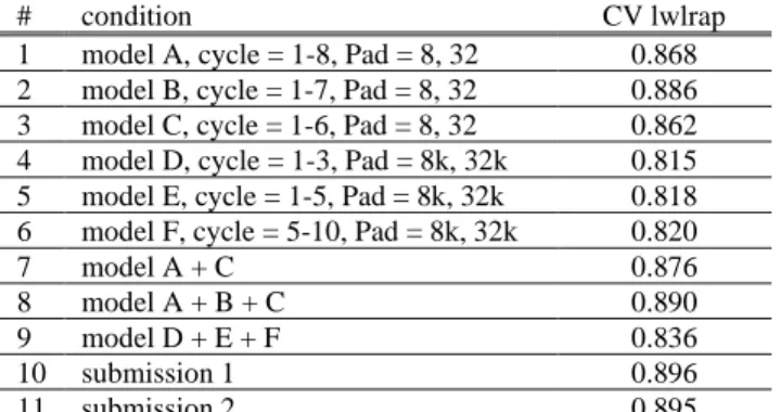
Table 3 shows the results of each model averaging condition.
# condition CV lwlrap
1 model A, cycle = 1-8, Pad = 8, 32 0.868
2 model B, cycle = 1-7, Pad = 8, 32 0.886
3 model C, cycle = 1-6, Pad = 8, 32 0.862
4 model D, cycle = 1-3, Pad = 8k, 32k 0.815 5 model E, cycle = 1-5, Pad = 8k, 32k 0.818 6 model F, cycle = 5-10, Pad = 8k, 32k 0.820
7 model A + C 0.876
8 model A + B + C 0.890
9 model D + E + F 0.836
10 submission 1 0.896
11 submission 2 0.895
Table 3: Comparison of model averaging. Pad: padding augmen-tation.
In every condition, we employed 5-fold CV averaging and Snap-shot Ensembles. By SnapSnap-shot Ensembles and padding augmenta-tion, the CV lwlrap increased +0.039 (Table 1 #4 and Table 3 #1). By cropping length averaging, the CV lwlrap increased +0.008 (Table 3 #1 and #7). By averaging models trained with log mel spectrogram and waveform, the CV lwlrap increased +0.008 (Ta-ble 3 #8 and #10).
On the public LB, submission 1 was ranked in 3rd place with a lwlrap score of 0.750. On the private LB, submission 2 was ranked in 4th place with a lwlrap score of 0.75787.
5. DISCUSSION
Our proposed methods showed meaningful results in the task, but there is room for improvement. First, we used shared convolution layers and separated FC layers for multitask learning, but we did not evaluate whether this model architecture is optimal. The opti-mized architecture may get more benefit from multitask learning.
Second, soft pseudo label failed to achieve reliable CV be-cause of implicit label leak from soft pseudo label. The procedure of soft pseudo label is very similar to model distillation [20], which uses averages of trained models’ predictions for training in the purpose of transferring knowledge of trained models to a sin-gle smaller model. Therefore, soft pseudo labels obtained from models trained with other CV folds have knowledge of labels of out-of-fold, and this can be label leaks. Establishing the way of reliable CV would make soft pseudo label more useful.
Third, we found that model averaging using models trained with different time length improves the score. This result suggests that training a single model with various time length would be successful and contributes to reducing the number of models.
Fourth, zero padding in training time makes models learn that there is a correlation between zero values and classes. Full-length prediction and padding augmentation can reduce this un-preferable bias. However, to avoid zero padding and concatenate several clones of the sound file instead may be more promising.
6. CONCLUSION
This paper describes our approach to the DCASE 2019 challenge Task 2, which is a difficult task because of multi-label and noisy label. We propose three strategies, multitask learning with noisy data, SSL with soft pseudo label and ensemble of cropping length averaging. By using these methods, our solution ranked in 4th place on the private LB.
7. REFERENCES
[1] E. Fonseca, J. Pons, X. Favory, F. Font, D. Bogdanov, A. Fer-raro, S. Oramas, A. Porter, and X. Serra, “Freesound datasets: a platform for the creation of open audio datasets,” in ISMIR 2017, 2017, pp. 486-493
[2] B. Thomee, D. A. Shamma, G. Friedland, B. Elizalde, K. Ni, D. Poland, D. Borth, and L.-J. Li, “YFCC100M: The New Data in Multimedia Research,” Commun ACM, 2016, 59(2), pp. 64–73.
[3] E. Fonseca, M. Plakal, F. Font, D. P. W. Ellis, and X. Serra, “Audio tagging with noisy labels and minimal supervision,” arXiv preprint arXiv:1906.02975, 2019.
[4] S. Ruder, “An Overview of Multi-Task Learning in Deep Neural Networks,” arXiv preprint arXiv:1706.05098, 2017. [5] T. Lee, T. Gong, S. Padhy, A. Rouditchenko, and A.
Ndirango, “Label-efficient audio classification through mul-titask learning and self-supervision,” in ICLR 2019 Workshop LLD, 2019.
[6] A. Oliver, A. Odena, C. Raffel, E. D. Cubuk, and I.J. Good-fellow, “Realistic Evaluation of Deep Semi-Supervised Learning Algorithms,” arXiv preprint arXiv: 1804.09170, 2018.
[7] D.-H. Lee, “Pseudo-label: The simple and efficient semi-su-pervised learning method for deep neural networks,” in ICML Workshop on Challenges in Representation Learning, 2013. [8] A. Tarvainen, and H. Valpola. “Mean teachers are better role
models: Weight-averaged consistency targets improve semi-supervised deep learning results,” arXiv preprint arXiv:1703.01780, 2017.
[9] D. Berthelot, N. Carlini, I. Goodfellow, N. Papernot, A. Oli-ver, and C. Raffel, “MixMatch: A Holistic Approach to Semi-Supervised Learning,” arXiv preprint arXiv:1905.02249, 2019.
[10]G. Huang, Y. Li, G. Pleiss, Z. Liu, J. E. Hopcroft, and K. Q. Weinberger, “Snapshot Ensembles: Train 1, get M for free,” arXiv preprint arXiv:1704.00109, 2017.
[11]H. Zhang, M. Cisse, Y. N. Dauphin, and D. Lopez-Paz, “mixup: Beyond empirical risk minimization,” arXiv preprint arXiv:1710.09412, 2017.
[12]I. Loshchilov, F. Hutter, “SGDR: Stochastic Gradient De-scent with Warm Restarts,” arXiv preprint arXiv:1608.03983, 2016.
[13]Y. Tokozume, Y. Ushiku, and T Harada, “Learning from Be-tween-class Examples for Deep Sound Recognition,” arXiv preprint arXiv:1711.10282, 2017.
[14]D. S. Park, W. Chan, Y. Zhang, C.-C. Chiu, B. Zoph, E. D. Cubuk, and Q. V. Le, “SpecAugment: A Simple Data Aug-mentation Method for Automatic Speech Recognition,” arXiv preprint arXiv:1904.08779, 2019.
[15]T. DeVries, and G. W. Taylor, “Improved Regularization of Convolutional Neural Networks with Cutout,” arXiv preprint arXiv:1708.04552, 2017.
[16]K. He, X. Zhang, S. Ren, and J. Sun, “Deep residual learning for image recognition,” in Proceedings of the IEEE confer-ence on computer vision and pattern recognition, 2016, pp. 770-778.
[17]J. Hu, L. Shen, and G. Sun, “Squeeze-and-Excitation Net-works,” arXiv preprint arXiv:1709.01507, 2017.
[18]N. Srivastava, G. Hinton, A. Krizhevsky, I. Sutskever, and R. Salakhutdinov, “Dropout: A Simple Way to Prevent Neural
Networks from Overfitting,” arXiv preprint arXiv: 1207.0580, 2015.
[19]D. P. Kingma, and J. Ba, “Adam: A method for stochastic optimization,” arXiv preprint arXiv:1412.6980, 2014. [20]G. Hinton, O. Vinyals, and J. Dean, “Distilling the
Knowledge in a Neural Network,” arXiv preprint arXiv: 1503.02531, 2015.