Chapter 4 Statistical Inference in Quality Control and Improvement. Statistical Quality Control (D. C. Montgomery)

Chapter 4

Statistical Inference in Quality Control and Improvement

許湘伶

Statistical Quality Control (D. C. Montgomery)

Sampling distribution I

I a random sample of size n: if it is selected so that the observations {xi} are i.i.d.

I x¯: central tendency

Sampling from a Normal Distribution I

Sampling from a Normal Distribution II

Sampling from a Normal Distribution III

Sampling from a Normal Distribution IV

I k→ ∞ ⇒ thet distribution is closely approximate N(0,1)

I Generallyk >30 I x1, . . . ,xn ∼N(µ, σ2) I ¯x∼N(µ,σ_n2) I (n−1)s 2 σ2 ∼χ 2 n−1 I ¯x⊥s2 ¯ x−µ s/√n ∼tn−1

Sampling from a Normal Distribution V

Sampling from a Normal Distribution VI

Sampling from a Bernoulli Distribution I

I x ∼ Ber(p) (p: the probability of success)

p(x) = ( p, x= 1 (1−p), x= 0 I x1, . . . ,xn ∼ Ber(p) x = n X i=1 x_i ∼ B(n,p) I E(¯x) =p, Var(¯x) = p(1_n−p)

Sampling from a Poisson Distribution I

I Linear combinations of Poisson r.v. are used in quality engineering work

I x_i i.∼ Pi.d (λi),i = 1, . . . ,m, {ai}: constants I m different types of defects

I The distribution of L=Pm_i=1aixi is not Poission unless all ai=1

Point Estimation of Process Parameters I

used to describe or model some critical-to-quality(關鍵質量

要素) control

I The parameters of the probability distributions are generally unknown

I A point estimator: a statistic that produces a single numerical value as the estimate of the unknown parameter Distribution Population parameter sample estimate

N(µ, σ2) µ ¯x N(µ, σ2) σ2 s2

P(λ) λ ¯x

Point Estimation of Process Parameters II

Properties

Important properties are required of good point estima-tors: 1. Unbiased: E(ˆθ) =θ 2. Minimum variance I E(¯x) =µ I Var(s2) =σ2 I E(s) =c4σ = 2 n−1 1/2 _Γ(n/2) Γ((n−2)/2)σ ⇒E s c4 =σ

Point Estimation of Process Parameters III

I Range method: to estimate the standard deviation

I x1. . . ,xn ∼N(µ, σ2)

The range sample: R= max

1≤i≤n(xi)−1≤mini≤n(xi) =xmax−xmin I The relative range: W = R_σ

E(W) =d₂ (d₂ : Appendix Table VI (2≤n≤25))

⇒ˆσ= R

Statistical Inference for a Single Sample I

I parameter estimation I hypothesis testing

I Statistical hypothesis: a statement about the values of the parameters of a probability distribution

Testing a hypothesis

I Null hypothesis (H0) and alternative hypothesis (H1)

I Testing statistics

I Type of errors

I Critical region (or rejection region)

I Reject of fail to reject theH₀ I Confidence interval

Statistical Inference for a Single Sample II

Type of errors

Hypothesis

H0is true H1is true Fail to rejectH0 Correct Decision Type II error (β)

RejectH0 Type I error (α) Correct Decision (1−β=Power)

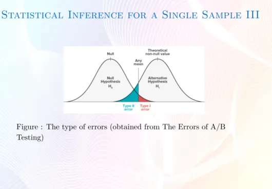
α=P{type I error}=P{rejectH0|H0 is true} (producer’s risk) β=P{type II error}=P{fail to rejectH0|H0is false} (consumer’s risk) Power = 1−β=P{rejectH0|H0 is false}

Statistical Inference for a Single Sample III

Figure : The type of errors (obtained from The Errors of A/B Testing)

Statistical Inference for a Single Sample IV

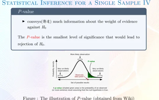
I conveys(傳達) much information about the weight of evidence againstH0

TheP-valueis the smallest level of significance that would lead to rejection ofH0.

Statistical Inference for a Single Sample V

Ex: Two-sided 100(1−α)% C.I.

construct an interval estimator of the meanµ

P{L≤µ≤U}= 1−α

100(1−α)% C.I. of µ: L ≤µ≤U

I One-sided lower 100(1−α)% C.I. : P{L≤µ}= 1−α

L ≤µ

I One-sided upper 100(1−α)% C.I. : P{µ≤U}= 1−α

Statistical Inference for a Single Sample VI

Hypothesis testing for a single sample:

I Inference on µ: variance knownorvariance unknown I Inference on σ2

I Inference on p (population proportion)

Statistical Inference for a Single Sample VII

Inference Sided Hypothesis Testing statistics Critical region 100(1−α)% C.I.

µ(σknown) Two-sided H0:µ=µ0 H1:µ6=µ0 Z0=x−µ¯ 0 σ/√n |Z0|>Zα/2 ¯x−Zα/2_√σ n≤µ≤¯x+Zα/2 σ √ n One-sided H0:µ=µ0 H1:µ > µ0 Z0>Zα x¯−Zα/2_√σ n≤µ H0:µ=µ0 H1:µ < µ0 Z0<−Zα x¯+Zα/2_√σ n≥µ µ(σunknown) Two-sided H0:µ=µ0 H1:µ6=µ0 t0=¯x−µ0 s/√n |t0|>tα/2,n−1 x¯−tα/2,n−1_√s n≤µ≤¯x+tα/2,n−1 s √ n One-sided H0:µ=µ0 H1:µ > µ0 t0>tα,n−1 x¯−tα,n−1_√s n≤µ H0:µ=µ0 H1:µ < µ0 t0<−tα,n−1 x¯+tα,n−1_√s n≥µ I z ∼N(0,1)⇒P(z>Z_α/2) =α/2 I t ∼tn−1⇒P(t>tα/2,n−1) =α/2

Statistical Inference for a Single Sample VIII

Test the hypothesis: the varianceof a normal distribution equals a constant

Inference Sided Hypothesis Testing statistics Critical region 100(1−α)% C.I.

σ Two-sided H0:σ=σ0 H1:σ6=σ0 χ2 0=(n−1)s 2 σ2 0 χ2 0> χ2α/2,n−1or χ2 0< χ21−α/2,n−1 (n−1)s2 χ2 α/2,n−1 ≤σ2_≤ (n−1)s2 χ2 1−α/2,n−1 One-sided H0:σ=σ0 H1:σ > σ0 χ2 0< χ21−α,n−1 σ2≤ (n−1)s 2 χ2 1−α,n−1 H0:σ=σ0 H1:σ < σ0 χ2 0> χ2α,n−1 (n−1)s 2 χ2 α,n−1 ≤σ2 I P(χ2_n−1>χ2α/2) =α/2 andP(χ2n−1>χ21−α/2) = 1−α/2

Statistical Inference for a Single Sample IX

Test the hypothesis: the proportionp of a population equals a standard value (p0)

I a random sample of n items is taken from the population

I x items in the sample belong to the class associated withp

I 二項分佈趨近至常態分佈

Inference Sided Hypothesis Testing statistics Critical region 100(1−α)% C.I. p Two-sided H0:p=p0 H1:p6=p0 Z0=      (x+0.5)−np0 √ np0(1−p0) ifx<np0 (x−0.5)−np0 √ np0(1−p0) ifx>np0 |Z0|>Zα/2 ˆp−Zα/2 q ˆ p(1−ˆp) n ≤p≤ˆp+Zα/2 q ˆ p(1−ˆp) n I pˆ= x_n

Statistical Inference for a Single Sample X

I n is large,p≥0.1⇒ the normal approximation to the binomial can be used

I n is small⇒ the binomial distribution ⇒C.I.

I n is large,p is small⇒ the Poisson distribution

Sample size Decisions I

H0 :µ=µ0 vs. H1 :µ6=µ0 ⇒Z₀ = ¯x−µ0 σ/√n ∼N(0,1) I Supposeµ1 =µ+δ, δ >0 (Under H1) Z₀= x¯−µ0 σ/√n ∼N( δ√n σ ,1)

I The type II error:

β = Φ Z_α/2−δ √ n σ ! −Φ −Z_α/2− δ √ n σ !

Sample size Decisions II

I β is a function of n, δ, α

I Specify α and design a test procedure maximize the power (⇒minimizeβ, a function of sample size.)

I Operating-characteristic (OC) curves(操作特性曲線):

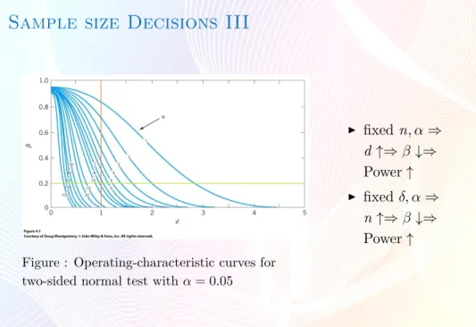
Sample size Decisions III

Figure : Operating-characteristic curves for two-sided normal test with α= 0.05

I fixedn, α⇒ d ↑⇒β ↓⇒ Power↑ I fixedδ, α⇒ n↑⇒β↓⇒ Power↑

Sample size Decisions IV

> library(pwr)

> pwr.t.test(n=25,d=0.75,sig.level=.01,alternative="greater",type ="one.sample")

One-sample t test power calculation

n = 25 d = 0.75 sig.level = 0.01 power = 0.8865127 alternative = greater > pwr.t.test(d=0.1/0.1,sig.level=0.05,power=0.85,type ="one.sample")

One-sample t test power calculation

n = 11.06276 d = 1 sig.level = 0.05

power = 0.85 alternative = two.sided

Inference for two samples I

I Inference for a difference inMeans: variance known or variance unknown

I Inference on the variances of two normal distributions

Inference for two samples II

Inference for two samples IV

Case 1:

σ2

1 =σ22=σ2 when variances unknown

I E(¯x₁−x¯₂) =µ1−µ2

I Var(¯x₁−x¯₂) =σ2_n11 +_n21

I Thepooled estimator ofσ2

sp2= (n1−1)s2 1+ (n2−1)s22 n1+n2−2 =ws 2 1+(1−w)s 2 2 (weighted average) I t test statistic: t = x¯1−¯x2−(µ1−µ2) s_pq_n11 + _n21 ∼t_n1+n2−2

Inference for two samples VI

Case 2:

σ₁26=σ₂2 when variances unknown

I The test statistic:

t₀∗ =x¯1−_rx¯2−(µ1−µ2) s₁2 n1 + s₂2 n2 ∼t_ν, ν = _s2 1 n1 + s2 2 n2 2 (s2 1/n1)2 n1−1 + (s2 2/n2)2 n2−1 −2

Inference for two samples VII

Paired data

I dj =x1j−x2j,j = 1, . . . ,n I Hypothesis:

H₀ :µd= 0⇔H0 :µ1 =µ2

I Thet test statistic:

t0= ¯

d

s_d/√n ∼tn−1 I RejectH₀ if|t₀|>t_α/2,n−1

Inference for two samples IX