A Handbook of Statistical Analyses
Using
R
CHAPTER 1
An Introduction to
R
1.1 What isR?
The Rsystem for statistical computing is an environment for data analysis and graphics. The root of Ris theS language, developed by John Chambers and colleagues (Becker et al., 1988, Chambers and Hastie, 1992, Chambers, 1998) at Bell Laboratories (formerly AT&T, now owned by Lucent Technolo-gies) starting in the 1960s. TheS language was designed and developed as a programming language for data analysis tasks but in fact it is a full-featured programming language in its current implementations.
The development of theRsystem for statistical computing is heavily influ-enced by the open source idea: The base distribution ofRand a large number of user contributed extensions are available under the terms of the Free Soft-ware Foundation’s GNU General Public License in source code form. This licence has two major implications for the data analyst working withR. The complete source code is available and thus the practitioner can investigate the details of the implementation of a special method, can make changes and can distribute modifications to colleagues. As a side-effect, theRsystem for statistical computing is available to everyone. All scientists, especially includ-ing those workinclud-ing in developinclud-ing countries, have access to state-of-the-art tools for statistical data analysis without additional costs. With the help of theR system for statistical computing, research really becomes reproducible when both the data and the results of all data analysis steps reported in a paper are available to the readers through anRtranscript file.Ris most widely used for teaching undergraduate and graduate statistics classes at universities all over the world because students can freely use the statistical computing tools.
The base distribution of Ris maintained by a small group of statisticians, theRDevelopment Core Team. A huge amount of additional functionality is implemented in add-on packages authored and maintained by a large group of volunteers. The main source of information about theRsystem is the world wide web with the official home page of theRproject being
http://www.R-project.org
All resources are available from this page: theRsystem itself, a collection of add-on packages, manuals, documentation and more.
The intention of this chapter is to give a rather informal introduction to basic concepts and data manipulation techniques for the R novice. Instead of a rigid treatment of the technical background, the most common tasks
are illustrated by practical examples and it is our hope that this will enable readers to get started without too many problems.
1.2 Installing R
TheRsystem for statistical computing consists of two major parts: the base system and a collection of user contributed add-on packages. TheRlanguage is implemented in the base system. Implementations of statistical and graphical procedures are separated from the base system and are organised in the form of packages. A package is a collection of functions, examples and documen-tation. The functionality of a package is often focused on a special statistical methodology. Both the base system and packages are distributed via the Com-prehensiveRArchive Network (CRAN) accessible under
http://CRAN.R-project.org 1.2.1 The Base System and the First Steps
The base system is available in source form and in precompiled form for various Unix systems, Windows platforms and Mac OS X. For the data analyst, it is sufficient to download the precompiled binary distribution and install it locally. Windows users follow the link
http://CRAN.R-project.org/bin/windows/base/release.htm download the corresponding file (currently named rw3021.exe), execute it locally and follow the instructions given by the installer.
Depending on the operating system,Rcan be started either by typing ‘R’ on the shell (Unix systems) or by clicking on the Rsymbol (as shown left) created by the installer (Windows). R comes without any frills and on start up shows simply a short introductory message including the version number and a prompt ‘>’:
R : Copyright 2015 The R Foundation for Statistical Computing Version 3.2.1 (2015-06-18), ISBN 3-900051-07-0
R is free software and comes with ABSOLUTELY NO WARRANTY. You are welcome to redistribute it under certain conditions. Type 'license()' or 'licence()' for distribution details. R is a collaborative project with many contributors. Type 'contributors()' for more information and
'citation()' on how to cite R or R packages in publications. Type 'demo()' for some demos, 'help()' for on-line help, or 'help.start()' for an HTML browser interface to help. Type 'q()' to quit R.
>
One can change the appearance of the prompt by > options(prompt = "R> ")
INSTALLINGR 3 and we will use the promptR>for the display of the code examples throughout this book.
Essentially, theRsystem evaluates commands typed on theRprompt and returns the results of the computations. The end of a command is indicated by the return key. Virtually all introductory texts onRstart with an example usingRas pocket calculator, and so do we:
R> x <- sqrt(25) + 2
This simple statement asks theRinterpreter to calculate√
25 and then to add 2. The result of the operation is assigned to anRobject with variable namex. The assignment operator<-binds the value of its right hand side to a variable name on the left hand side. The value of the objectxcan be inspected simply by typing
R> x
[1] 7
which, implicitly, calls theprintmethod: R> print(x)
[1] 7
1.2.2 Packages
The base distribution already comes with some high-priority add-on packages, namely
Matrix boot lattice mgcv rpart survival KernSmooth MASS base class cluster codetools compiler datasets foreign grDevices graphics grid methods nlme nnet parallel spatial splines stats stats4 tcltk tools utils
The packages listed here implement standard statistical functionality, for ex-ample linear models, classical tests, a huge collection of high-level plotting functions or tools for survival analysis; many of these will be described and used in later chapters.
Packages not included in the base distribution can be installed directly from theRprompt. At the time of writing this chapter, 6899 user contributed packages covering almost all fields of statistical methodology were available.
Given that an Internet connection is available, a package is installed by supplying the name of the package to the function install.packages. If, for example, add-on functionality for robust estimation of covariance matrices via sandwich estimators is required (for example in Chapter??), thesandwich package (Zeileis,2004) can be downloaded and installed via
The package functionality is available after attachingthe package by R> library("sandwich")
A comprehensive list of available packages can be obtained from http://CRAN.R-project.org/src/contrib/PACKAGES.html
Note that on Windows operating systems, precompiled versions of packages are downloaded and installed. In contrast, packages are compiled locally before they are installed on Unix systems.
1.3 Help and Documentation
Roughly, three different forms of documentation for the Rsystem for statis-tical computing may be distinguished: online help that comes with the base distribution or packages, electronic manuals and publications work in the form of books etc.
The help system is a collection of manual pages describing each user-visible function and data set that comes withR. A manual page is shown in a pager or web browser when the name of the function we would like to get help for is supplied to thehelpfunction
R> help("mean") or, for short, R> ?mean
Each manual page consists of a general description, the argument list of the documented function with a description of each single argument, information about the return value of the function and, optionally, references, cross-links and, in most cases, executable examples. The functionhelp.searchis helpful for searching within manual pages. An overview on documented topics in an add-on package is given, for example for the sandwichpackage, by
R> help(package = "sandwich")
Often a package comes along with an additional document describing the pack-age functionality and giving examples. Such a document is called a vignette (Leisch, 2003, Gentleman, 2005). The sandwich package vignette is opened using
R> vignette("sandwich", package = "sandwich")
More extensive documentation is available electronically from the collection of manuals at
http://CRAN.R-project.org/manuals.html
For the beginner, at least the first and the second document of the following four manuals (R Development Core Team,2005a,b,c,d) are mandatory: An Introduction to R: A more formal introduction to data analysis with
Rthan this chapter.
R Data Import/Export: A very useful description of how to read and write various external data formats.
DATA OBJECTS INR 5 R Installation and Administration: Hints for installingRon special
plat-forms.
Writing R Extensions: The authoritative source on how to write R pro-grams and packages.
Both printed and online publications are available, the most important ones are ‘Modern Applied Statistics with S’ (Venables and Ripley, 2002), ‘Intro-ductory Statistics withR’ (Dalgaard,2002), ‘RGraphics’ (Murrell,2005) and theRNewsletter, freely available from
http://CRAN.R-project.org/doc/Rnews/
In case the electronically available documentation and the answers to fre-quently asked questions (FAQ), available from
http://CRAN.R-project.org/faqs.html
have been consulted but a problem or question remains unsolved, ther-help email list is the right place to get answers to well-thought-out questions. It is helpful to read the posting guide
http://www.R-project.org/posting-guide.html before starting to ask.
1.4 Data Objects in R
The data handling and manipulation techniques explained in this chapter will be illustrated by means of a data set of 2000 world leading companies, the Forbes 2000 list for the year 2004 collected by ‘Forbes Magazine’. This list is originally available from
http://www.forbes.com
and, as an R data object, it is part of the HSAUR package (Source: From Forbes.com, New York, New York, 2004. With permission.). In a first step, we make the data available for computations withinR. Thedatafunction searches for data objects of the specified name ("Forbes2000")in the package specified via thepackageargument and, if the search was successful, attaches the data object to the global environment:
R> data("Forbes2000", package = "HSAUR") R> ls()
[1] "Forbes2000" "a" "book" "ch" [5] "refs" "s" "x"
The output of thelsfunction lists the names of all objects currently stored in the global environment, and, as the result of the previous command, a variable namedForbes2000is available for further manipulation. The variablexarises from the pocket calculator example in Subsection1.2.1.
As one can imagine, printing a list of 2000 companies via R> print(Forbes2000)
rank name country category sales 1 1 Citigroup United States Banking 94.71 2 2 General Electric United States Conglomerates 134.19 3 3 American Intl Group United States Insurance 76.66
profits assets marketvalue 1 17.85 1264.03 255.30 2 15.59 626.93 328.54 3 6.46 647.66 194.87 ...
will not be particularly helpful in gathering some initial information about the data; it is more useful to look at a description of their structure found by using the following command
R> str(Forbes2000)
'data.frame': 2000 obs. of 8 variables: $ rank : int 1 2 3 4 5 ...
$ name : chr "Citigroup" "General Electric" ...
$ country : Factor w/ 61 levels "Africa","Australia",..: 60 60 60 60 56 ... $ category : Factor w/ 27 levels "Aerospace & defense",..: 2 6 16 19 19 ... $ sales : num 94.7 134.2 ...
$ profits : num 17.9 15.6 ... $ assets : num 1264 627 ... $ marketvalue: num 255 329 ...
The output of thestrfunction tells us thatForbes2000is an object of class
data.frame, the most important data structure for handling tabular statistical
data inR. As expected, information about 2000 observations, i.e., companies, are stored in this object. For each observation, the following eight variables are available:
rank: the ranking of the company, name: the name of the company,
country: the country the company is situated in,
category: a category describing the products the company produces, sales: the amount of sales of the company in billion US dollars, profits: the profit of the company in billion US dollars, assets: the assets of the company in billion US dollars,
marketvalue: the market value of the company in billion US dollars. A similar but more detailed description is available from the help page for the Forbes2000object:
R> help("Forbes2000") or
R> ?Forbes2000
All information provided by strcan be obtained by specialised functions as well and we will now have a closer look at the most important of these.
TheRlanguage is an object-oriented programming language, so every object is an instance of a class. The name of the class of an object can be determined by
DATA OBJECTS INR 7
[1] "data.frame"
Objects of classdata.frame represent data the traditional table oriented way. Each row is associated with one single observation and each column corre-sponds to one variable. The dimensions of such a table can be extracted using thedimfunction
R> dim(Forbes2000)
[1] 2000 8
Alternatively, the numbers of rows and columns can be found using R> nrow(Forbes2000)
[1] 2000
R> ncol(Forbes2000)
[1] 8
The results of both statements show that Forbes2000 has 2000 rows, i.e., observations, the companies in our case, with eight variables describing the observations. The variable names are accessible from
R> names(Forbes2000)
[1] "rank" "name" "country" "category" [5] "sales" "profits" "assets" "marketvalue"
The values of single variables can be extracted from theForbes2000 object by their names, for example the ranking of the companies
R> class(Forbes2000[,"rank"])
[1] "integer"
is stored as an integer variable. Brackets[]always indicate a subset of a larger object, in our case a single variable extracted from the whole table. Because
data.frames have two dimensions, observations and variables, the comma is
required in order to specify that we want a subset of the second dimension, i.e., the variables. The rankings for all 2000 companies are represented in a
vector structure the length of which is given by
R> length(Forbes2000[,"rank"])
[1] 2000
A vector is the elementary structure for data handling in R and is a set of
simple elements, all being objects of the same class. For example, a simple vector of the numbers one to three can be constructed by one of the following commands R> 1:3 [1] 1 2 3 R> c(1,2,3) [1] 1 2 3 R> seq(from = 1, to = 3, by = 1) [1] 1 2 3
The unique names of all 2000 companies are stored in a character vector R> class(Forbes2000[,"name"])
[1] "character"
R> length(Forbes2000[,"name"])
[1] 2000
and the first element of this vector is R> Forbes2000[,"name"][1]
[1] "Citigroup"
Because the companies are ranked, Citigroup is the world’s largest company according to the Forbes 2000 list. Further details on vectors and subsetting are given in Section1.6.
Nominal measurements are represented byfactor variables inR, such as the category of the company’s business segment
R> class(Forbes2000[,"category"])
[1] "factor"
Objects of class factor and character basically differ in the way their values are stored internally. Each element of a vector of classcharacter is stored as a
character variable whereas an integer variable indicating the level of afactor
is saved forfactor objects. In our case, there are R> nlevels(Forbes2000[,"category"])
[1] 27
different levels, i.e., business categories, which can be extracted by R> levels(Forbes2000[,"category"])
[1] "Aerospace & defense" [2] "Banking"
[3] "Business services & supplies" ...
As a simple summary statistic, the frequencies of the levels of such a factor variable can be found from
R> table(Forbes2000[,"category"])
Aerospace & defense Banking
19 313
Business services & supplies 70 ...
The sales, assets, profits and market value variables are of type numeric, the natural data type for continuous or discrete measurements, for example R> class(Forbes2000[,"sales"])
[1] "numeric"
and simple summary statistics such as the mean, median and range can be found from
DATA IMPORT AND EXPORT 9 R> median(Forbes2000[,"sales"]) [1] 4.365 R> mean(Forbes2000[,"sales"]) [1] 9.69701 R> range(Forbes2000[,"sales"]) [1] 0.01 256.33
Thesummarymethod can be applied to a numeric vector to give a set of useful summary statistics namely the minimum, maximum, mean, median and the 25% and 75% quartiles; for example
R> summary(Forbes2000[,"sales"])
Min. 1st Qu. Median Mean 3rd Qu. Max. 0.010 2.018 4.365 9.697 9.548 256.300
1.5 Data Import and Export
In the previous section, the data from the Forbes 2000 list of the world’s largest companies were loaded intoRfrom theHSAUR package but we will now ex-plore practically more relevant ways to import data into the Rsystem. The most frequent data formats the data analyst is confronted with are comma sep-arated files,Excelspreadsheets, files inSPSSformat and a variety ofSQLdata base engines. Querying data bases is a non-trivial task and requires additional knowledge about querying languages and we therefore refer to the ‘RData Im-port/Export’ manual – see Section 1.3. We assume that a comma separated file containing the Forbes 2000 list is available as Forbes2000.csv (such a file is part of theHSAURsource package in directoryHSAUR/inst/rawdata). When the fields are separated by commas and each row begins with a name (a text format typically created byExcel), we can read in the data as follows using theread.table function
R> csvForbes2000 <- read.table("Forbes2000.csv", + header = TRUE, sep = ",", row.names = 1)
The argumentheader = TRUEindicates that the entries in the first line of the text file"Forbes2000.csv"should be interpreted as variable names. Columns are separated by a comma (sep = ","), users of continental versions of Excel should take care of the character symbol coding for decimal points (by default dec = "."). Finally, the first column should be interpreted as row names but not as a variable (row.names = 1). Alternatively, the functionread.csvcan be used to read comma separated files. The functionread.table by default guesses the class of each variable from the specified file. In our case, character variables are stored as factors
R> class(csvForbes2000[,"name"])
[1] "factor"
which is only suboptimal since the names of the companies are unique. How-ever, we can supply the types for each variable to thecolClassesargument
R> csvForbes2000 <- read.table("Forbes2000.csv", + header = TRUE, sep = ",", row.names = 1,
+ colClasses = c("character", "integer", "character", + "factor", "factor", "numeric", "numeric", "numeric", + "numeric"))
R> class(csvForbes2000[,"name"])
[1] "character"
and check if this object is identical with our previous Forbes 2000 list object R> all.equal(csvForbes2000, Forbes2000)
[1] "Component \"name\": 23 string mismatches"
The argument colClasses expects a character vector of length equal to the number of columns in the file. Such a vector can be supplied by thecfunction that combines the objects given in the parameter list into avector
R> classes <- c("character", "integer", "character", "factor", + "factor", "numeric", "numeric", "numeric", "numeric") R> length(classes)
[1] 9
R> class(classes)
[1] "character"
An R interface to the open data base connectivity standard (ODBC) is available in packageRODBC and its functionality can be used to assessExcel andAccess files directly:
R> library("RODBC")
R> cnct <- odbcConnectExcel("Forbes2000.xls")
R> sqlQuery(cnct, "select * from \"Forbes2000\\$\"")
The functionodbcConnectExcelopens a connection to the specifiedExcelor Accessfile which can be used to sendSQLqueries to the data base engine and retrieve the results of the query.
Files inSPSSformat are read in a way similar to reading comma separated files, using the function read.spss from packageforeign (which comes with the base distribution).
Exporting data fromRis now rather straightforward. A comma separated file readable byExcelcan be constructed from adata.frame object via R> write.table(Forbes2000, file = "Forbes2000.csv", sep = ",",
+ col.names = NA)
The functionwrite.csvis one alternative and the functionality implemented in theRODBC package can be used to write data directly intoExcel spread-sheets as well.
Alternatively, when data should be saved for later processing in Ronly,R objects of arbitrary kind can be stored into an external binary file via R> save(Forbes2000, file = "Forbes2000.rda")
BASIC DATA MANIPULATION 11 where the extension.rda is standard. We can get the file names of all files with extension.rdafrom the working directory
R> list.files(pattern = "\\.rda")
[1] "Forbes2000.rda"
and we can load the contents of the file intoRby R> load("Forbes2000.rda")
1.6 Basic Data Manipulation
The examples shown in the previous section have illustrated the importance of
data.frames for storing and handling tabular data inR. Internally, adata.frame
is alist of vectors of a common lengthn, the number of rows of the table. Each
of those vectors represents the measurements of one variable and we have seen that we can access such a variable by its name, for example the names of the companies
R> companies <- Forbes2000[,"name"]
Of course, the companies vector is of class character and of length 2000. A subset of the elements of the vectorcompaniescan be extracted using the[] subset operator. For example, the largest of the 2000 companies listed in the Forbes 2000 list is
R> companies[1]
[1] "Citigroup"
and the top three companies can be extracted utilising an integer vector of the numbers one to three:
R> 1:3
[1] 1 2 3
R> companies[1:3]
[1] "Citigroup" "General Electric" [3] "American Intl Group"
In contrast to indexing with positive integers, negative indexing returns all elements which arenotpart of the index vector given in brackets. For example, all companies except those with numbers four to two-thousand, i.e., the top three companies, are again
R> companies[-(4:2000)]
[1] "Citigroup" "General Electric" [3] "American Intl Group"
The complete information about the top three companies can be printed in a similar way. Becausedata.frames have a concept of rows and columns, we need to separate the subsets corresponding to rows and columns by a comma. The statement
name sales profits assets 1 Citigroup 94.71 17.85 1264.03 2 General Electric 134.19 15.59 626.93 3 American Intl Group 76.66 6.46 647.66
extracts the variablesname,sales,profitsandassetsfor the three largest companies. Alternatively, a single variable can be extracted from adata.frame by
R> companies <- Forbes2000$name
which is equivalent to the previously shown statement R> companies <- Forbes2000[,"name"]
We might be interested in extracting the largest companies with respect to an alternative ordering. The three top selling companies can be computed along the following lines. First, we need to compute the ordering of the com-panies’ sales
R> order_sales <- order(Forbes2000$sales)
which returns the indices of the ordered elements of the numeric vectorsales. Consequently the three companies with the lowest sales are
R> companies[order_sales[1:3]]
[1] "Custodia Holding" "Central European Media" [3] "Minara Resources"
The indices of the three top sellers are the elements 1998,1999 and 2000 of
the integer vectororder_sales
R> Forbes2000[order_sales[c(2000, 1999, 1998)],
+ c("name", "sales", "profits", "assets")]
name sales profits assets 10 Wal-Mart Stores 256.33 9.05 104.91 5 BP 232.57 10.27 177.57 4 ExxonMobil 222.88 20.96 166.99
Another way of selecting vector elements is the use of a logical vector being TRUE when the corresponding element is to be selected andFALSEotherwise. The companies with assets of more than 1000 billion US dollars are
R> Forbes2000[Forbes2000$assets > 1000,
+ c("name", "sales", "profits", "assets")]
name sales profits assets 1 Citigroup 94.71 17.85 1264.03 9 Fannie Mae 53.13 6.48 1019.17 403 Mizuho Financial 24.40 -20.11 1115.90
where the expression Forbes2000$assets > 1000 indicates a logical vector of length 2000 with
R> table(Forbes2000$assets > 1000)
FALSE TRUE 1997 3
elements being either FALSEor TRUE. In fact, for some of the companies the measurement of the profits variable are missing. In R, missing values are treated by a special symbol,NA, indicating that this measurement is not avail-able. The observations with profit information missing can be obtained via
SIMPLE SUMMARY STATISTICS 13 R> na_profits <- is.na(Forbes2000$profits) R> table(na_profits) na_profits FALSE TRUE 1995 5 R> Forbes2000[na_profits,
+ c("name", "sales", "profits", "assets")]
name sales profits assets 772 AMP 5.40 NA 42.94 1085 HHG 5.68 NA 51.65 1091 NTL 3.50 NA 10.59 1425 US Airways Group 5.50 NA 8.58 1909 Laidlaw International 4.48 NA 3.98
where the functionis.nareturns a logical vector beingTRUEwhen the corre-sponding element of the supplied vector isNA. A more comfortable approach is available when we want to remove all observations with at least one miss-ing value from a data.frame object. The function complete.cases takes a
data.frame and returns a logical vector being TRUE when the corresponding
observation does not contain any missing value: R> table(complete.cases(Forbes2000))
FALSE TRUE 5 1995
Subsetting data.frames driven by logical expressions may induce a lot of typing which can be avoided. Thesubsetfunction takes adata.frame as first argument and a logical expression as second argument. For example, we can select a subset of the Forbes 2000 list consisting of all companies situated in the United Kingdom by
R> UKcomp <- subset(Forbes2000, country == "United Kingdom") R> dim(UKcomp)
[1] 137 8
i.e., 137 of the 2000 companies are from the UK. Note that it is not neces-sary to extract the variablecountryfrom the data.frame Forbes2000when formulating the logical expression.
1.7 Simple Summary Statistics
Two functions are helpful for getting an overview about Robjects: strand summary, where str is more detailed about data types andsummary gives a collection of sensible summary statistics. For example, applying thesummary method to theForbes2000data set,
R> summary(Forbes2000) results in the following output
rank name country Min. : 1.0 Length:2000 United States :751 1st Qu.: 500.8 Class :character Japan :316 Median :1000.5 Mode :character United Kingdom:137 Mean :1000.5 Germany : 65
3rd Qu.:1500.2 France : 63 Max. :2000.0 Canada : 56 (Other) :612 category sales
Banking : 313 Min. : 0.010 Diversified financials: 158 1st Qu.: 2.018 Insurance : 112 Median : 4.365 Utilities : 110 Mean : 9.697 Materials : 97 3rd Qu.: 9.547 Oil & gas operations : 90 Max. :256.330 (Other) :1120
profits assets marketvalue Min. :-25.8300 Min. : 0.270 Min. : 0.02 1st Qu.: 0.0800 1st Qu.: 4.025 1st Qu.: 2.72 Median : 0.2000 Median : 9.345 Median : 5.15 Mean : 0.3811 Mean : 34.042 Mean : 11.88 3rd Qu.: 0.4400 3rd Qu.: 22.793 3rd Qu.: 10.60 Max. : 20.9600 Max. :1264.030 Max. :328.54 NA's :5
From this output we can immediately see that most of the companies are situated in the US and that most of the companies are working in the banking sector as well as that negative profits, or losses, up to 26 billion US dollars occur.
Internally,summaryis a so-calledgeneric functionwith methods for a multi-tude of classes, i.e.,summarycan be applied to objects of different classes and will report sensible results. Here, we supply a data.frame object to summary where it is natural to applysummaryto each of the variables in thisdata.frame. Because adata.frameis alist with each variable being an element of thatlist, the same effect can be achieved by
R> lapply(Forbes2000, summary)
The members of the apply family help to solve recurring tasks for each element of adata.frame,matrix,list or for each level of a factor. It might be interesting to compare the profits in each of the 27 categories. To do so, we first compute the median profit for each category from
R> mprofits <- tapply(Forbes2000$profits,
+ Forbes2000$category, median, na.rm = TRUE) a command that should be read as follows. For each level of the factor cat-egory, determine the corresponding elements of the numeric vectorprofits and supply them to the median function with additional argumentna.rm = TRUE. The latter one is necessary because profits contains missing values which would lead to a non-sensible result of themedianfunction
R> median(Forbes2000$profits)
[1] NA
The three categories with highest median profit are computed from the vector of sorted median profits
R> rev(sort(mprofits))[1:3]
Oil & gas operations Drugs & biotechnology
0.35 0.35
Household & personal products 0.31
ORGANISING AN ANALYSIS 15 where rev rearranges the vector of median profits sorted from smallest to largest. Of course, we can replace the median function with mean or what-ever is appropriate in the call totapply. In our situation,meanis not a good choice, because the distributions of profits or sales are naturally skewed. Sim-ple graphical tools for the inspection of distributions are introduced in the next section.
1.7.1 Simple Graphics
The degree of skewness of a distribution can be investigated by constructing histograms using thehistfunction. (More sophisticated alternatives such as smooth density estimates will be considered in Chapter??.) For example, the code for producing Figure 1.1 first divides the plot region into two equally spaced rows (thelayoutfunction) and then plots the histograms of the raw market values in the upper part using the hist function. The lower part of the figure depicts the histogram for the log transformed market values which appear to be more symmetric.
Bivariate relationships of two continuous variables are usually depicted as scatterplots. In R, regression relationships are specified by so-called model
formulae which, in a simple bivariate case, may look like
R> fm <- marketvalue ~ sales R> class(fm)
[1] "formula"
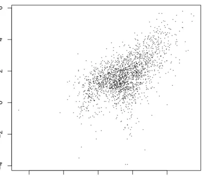
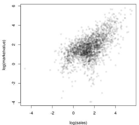
with the dependent variable on the left hand side and the independent vari-able on the right hand side. The tilde separates left and right hand side. Such a model formula can be passed to a model function (for example to the linear model function as explained in Chapter ??). The plot generic function im-plements aformula method as well. Because the distributions of both market value and sales are skewed we choose to depict their logarithms. A raw scat-terplot of 2000 data points (Figure1.2) is rather uninformative due to areas with very high density. This problem can be avoided by choosing a transpar-ent color for the dots (currtranspar-ently only possible with the PDF graphics device) as shown in Figure1.3.
If the independent variable is a factor, a boxplot representation is a natural choice. For four selected countries, the distributions of the logarithms of the market value may be visually compared in Figure1.4. Here, the width of the boxes are proportional to the square root of the number of companies for each country and extremely large or small market values are depicted by single points.
1.8 Organising an Analysis
Although it is possible to perform an analysis typing all commands directly on theRprompt it is much more comfortable to maintain a separate text file collecting all steps necessary to perform a certain data analysis task. Such
R> layout(matrix(1:2, nrow = 2)) R> hist(Forbes2000$marketvalue) R> hist(log(Forbes2000$marketvalue)) Histogram of Forbes2000$marketvalue Forbes2000$marketvalue Frequency 0 50 100 150 200 250 300 350 0 1000 Histogram of log(Forbes2000$marketvalue) log(Forbes2000$marketvalue) Frequency −4 −2 0 2 4 6 0 400 800
Figure 1.1 Histograms of the market value and the logarithm of the market value for the companies contained in the Forbes 2000 list.
anRtranscript file, for exampleanalysis.Rcreated with your favourite text editor, can be sourced into Rusing thesourcecommand
R> source("analysis.R", echo = TRUE)
When all steps of a data analysis, i.e., data preprocessing, transformations, simple summary statistics and plots, model building and inference as well as reporting, are collected in such an R transcript file, the analysis can be reproduced at any time, maybe with modified data as it frequently happens in our consulting practice.
SUMMARY 17 R> plot(log(marketvalue) ~ log(sales), data = Forbes2000,
+ pch = ".") −4 −2 0 2 4 −4 −2 0 2 4 6 log(sales) log(mar k etv alue)
Figure 1.2 Raw scatterplot of the logarithms of market value and sales.
1.9 Summary
Reading data intoRis possible in many different ways, including direct con-nections to data base engines. Tabular data are handled bydata.frames inR, and the usual data manipulation techniques such as sorting, ordering or sub-setting can be performed by simpleRstatements. An overview on data stored
in adata.frame is given mainly by two functions:summary and str. Simple
graphics such as histograms and scatterplots can be constructed by applying the appropriate R functions (hist and plot) and we shall give many more examples of these functions and those that produce more interesting graphics in later chapters.
R> plot(log(marketvalue) ~ log(sales), data = Forbes2000, + col = rgb(0,0,0,0.1), pch = 16)
Figure 1.3 Scatterplot with transparent shading of points of the logarithms of market value and sales.
Exercises
Ex. 1.1 Calculate the median profit for the companies in the United States and the median profit for the companies in the UK, France and Germany. Ex. 1.2 Find all German companies with negative profit.
Ex. 1.3 Which business category are most of the companies situated at the Bermuda island working in?
Ex. 1.4 For the 50 companies in the Forbes data set with the highest profits, plot sales against assets (or some suitable transformation of each variable), labelling each point with the appropriate country name which may need
SUMMARY 19 R> boxplot(log(marketvalue) ~ country, data =
+ subset(Forbes2000, country %in% c("United Kingdom", + "Germany", "India", "Turkey")),
+ ylab = "log(marketvalue)", varwidth = TRUE)
● ● ● ● ● ● ●
Germany India Turkey United Kingdom
−2 0 2 4 log(mar k etv alue)
Figure 1.4 Boxplots of the logarithms of the market value for four selected coun-tries, the width of the boxes is proportional to the square-roots of the number of companies.
to be abbreviated (using abbreviate) to avoid making the plot look too ‘messy’.
Ex. 1.5 Find the average value of sales for the companies in each country in the Forbes data set, and find the number of companies in each country with profits above 5 billion US dollars.
Bibliography
Becker, R. A., Chambers, J. M., and Wilks, A. R. (1988),The New S
Lan-guage, London, UK: Chapman & Hall.
Chambers, J. M. (1998),Programming with Data, New York, USA: Springer. Chambers, J. M. and Hastie, T. J. (1992), Statistical Models in S, London,
UK: Chapman & Hall.
Dalgaard, P. (2002),Introductory Statistics with R, New York: Springer. Gentleman, R. (2005), “Reproducible research: A bioinformatics case study,”
Statistical Applications in Genetics and Molecular Biology, 4, URLhttp:
//www.bepress.com/sagmb/vol4/iss1/art2, article 2.
Leisch, F. (2003), “Sweave, Part II: Package vignettes,”R News, 3, 21–24, URLhttp://CRAN.R-project.org/doc/Rnews/.
Murrell, P. (2005), R Graphics, Boca Raton, Florida, USA: Chapman & Hall/CRC.
R Development Core Team (2005a),An Introduction to R, R Foundation for Statistical Computing, Vienna, Austria, URLhttp://www.R-project.org, ISBN 3-900051-12-7.
R Development Core Team (2005b),R Data Import/Export, R Foundation for Statistical Computing, Vienna, Austria, URLhttp://www.R-project.org, ISBN 3-900051-10-0.
R Development Core Team (2005c), R Installation and Administration, R Foundation for Statistical Computing, Vienna, Austria, URLhttp://www. R-project.org, ISBN 3-900051-09-7.
R Development Core Team (2005d),Writing R Extensions, R Foundation for Statistical Computing, Vienna, Austria, URLhttp://www.R-project.org, ISBN 3-900051-11-9.
Venables, W. N. and Ripley, B. D. (2002), Modern Applied Statistics with S, Springer, 4th edition, URLhttp://www.stats.ox.ac.uk/pub/MASS4/, ISBN 0-387-95457-0.
Zeileis, A. (2004), “Econometric computing with HC and HAC covariance matrix estimators,”Journal of Statistical Software, 11, 1–17, URL http: //jstatsoft.org/v11/i10/.